Public and Private Inputs in Aggregate Production and Growth: A Cross-country Efficiency Approach

(1)

António Afonso & Miguel St. Aubyn

Public and Private Inputs in Aggregate Production and

Growth: A Cross-country Efficiency Approach

WP 09/2010/DE/UECE ___________________________________________________________________

Department of Economics

W

ORKING

P

APERS

ISSN Nº 0874-4548

School of Economics and Management

(2)

Public and Private Inputs in Aggregate

Production and Growth: A

Cross-country Efficiency Approach

*

António Afonso

$ #

and Miguel St. Aubyn

#

January 2010

Abstract

In a cross section of OECD countries we replace the macroeconomic production function by a production possibility frontier, TFP being the composite effect of efficiency scores and possibility frontier changes. We consider, for the periods 1970, 1980, 1990, 2000, one output: GDP per worker; three inputs: human capital, public physical capital per worker and private physical capital per worker. We use a semi-parametric analysis, computing Malmquist productivity indexes, and we also resort to stochastic frontier analysis. Results show that private capital is important for growth, although public and human capital also contribute positively. A governance indicator, a non-discretionary input, explains inefficiency. Better governance helps countries to achieve a better performance. Non-parametric and parametric results coincide rather closely on the countries movements vis-à-vis the possibility frontier, and on their relative distances to the frontier.

JEL: C14, D24, H50, O47

Keywords: economic growth, public spending, efficiency, Malmquist index.

*

We are grateful to Jürgen von Hagen, Geraint Johnes, Martin Larch, Ad van Riet, Emmanuel Thanassoulis, participants at the DG ECFIN Workshop “The Quality of Public Finances and Economic Growth” (Brussels), at the 3rd Meeting of the Portuguese Economic Journal (Funchal), at the 3rd Workshop on Efficiency and Productivity Analysis (Porto), and an anonymous ECB WPS referee for helpful comments and suggestions. The opinions expressed herein are those of the authors and do not necessarily reflect those of the ECB or the Eurosystem.

$

European Central Bank, Directorate General Economics, Kaiserstraße 29, D-60311 Frankfurt am Main, Germany, email: antonio.afonso@ecb.europa.eu.

#

(3)

Contents

Non-technical summary ... 3

1. Introduction ... 5

2. Literature ... 8

3. Methodology ... 10

3.1. DEA and the Malmquist index ... 10

3.2. Stochastic frontier ... 14

4. Empirical analysis ... 15

4.1. Data ... 15

4.2. Non-parametric analysis ... 16

4.3. Parametric analysis ... 20

5. Conclusion ... 22

References ... 24

Appendix – Data sources... 27

Annex – Additional estimates ... 34

Non-technical summary

(4)

human capital, public physical capital per worker and private physical capital per worker. We use a semi-parametric analysis, computing Malmquist productivity indexes, and we also resort to stochastic frontier analysis.

Results show that: i) private capital is important for growth, and contributes in a significant manner to input accumulation; ii) public and human capital contribution is usually estimated as positive, but, depending on the specification, it was not always significant from a statistical point a view; iii) a governance indicator (government effectiveness), a non-discretionary input, explains inefficiency. Our results also support the idea that better governance helps countries to achieve a better performance and to operate closer to the production possibility frontier.

Deterministic and stochastic estimation methods provide similar results and conclusions. Notably, non-parametric and parametric results coincide rather closely on the countries movements vis-à-vis the possibility frontier and on their relative distances to the frontier. The number of countries that can be nominated as efficient was stable throughout the period, with six or seven countries usually on the frontier (Belgium, Canada, Spain, Italy, Japan, Portugal, and the USA). In addition, it is worthwhile noticing the steady improvement in (technical) efficiency throughout the time sample for such countries as Ireland, Norway, and Finland, with the first two countries reaching the efficiency frontier in 2000, and depicting the biggest TFP change in that period. An opposite development can be seen for the case of Japan that shifts away from the efficiency frontier between 1970 and 2000.

Our estimations imply that policy may matter for growth by at least three different channels. One is public investment. The public capital elasticity is imprecisely estimated. These estimates and their variability are consistent with other results available in the literature concerning the effects of public investment across countries. The policy content of these results has to be seen with caution – macroeconomic analysis can be no substitute for the careful evaluation of each public project on its own merits.

(5)

Finally, our results are also consistent with the importance of human capital formation for growth. There is some evidence of a positive macroeconomic return for human capital investment. Some countries in our sample, even if they are close to or at the efficiency frontier (Portugal, Spain), are probably limited in their growth prospects by their relative human capital scarcity.

1. Introduction

The empirics of growth are generally based on an aggregate production function

approach. In a typical framework, production depends on labour, physical capital,

human capital and total factor productivity (TFP). Total factor productivity is an

(6)

specifying a production function (e.g. of a Cobb-Douglas variety); ii) estimating or

calibrating the production function parameters; iii) and obtaining TFP as a Solow

residual, the change in production that is not explained by changes in production

factors.

The researcher is very often interested in TFP estimates. For example, one may

be interested in how TFP differs across countries in response to different environments

likely to affect growth (policies, governance, institutions...), and also in how TFP

changes throughout time. However, TFP estimates obtained in the manner described

above heavily depend on the assumptions about the production function.

In this paper we replace the macroeconomic production function by a production

possibility frontier. TFP is computed as the composite effect of efficiency scores and

possibility frontier changes. The efficiency score provides information on how far away

a country is from the frontier, given the inputs it is using in production. We will

consider, in a cross section of countries, one output: GDP per worker; three inputs:

human capital, public physical capital per worker and private physical per worker; and

an environmental variable (a non-discretionary input), related to public policy, under the

form of a governance indicator. These variables are usually useful to explain changes in

country efficiency scores and therefore in the distance to the frontier.

We use two different methods to estimate the production possibility frontier.

Firstly, we apply the semi-parametric analysis with non-discretionary inputs in a

similar manner as in Afonso and St. Aubyn (2006). This approach has one important

advantage – the number of a priori assumptions is much smaller, as there is no need to

specify a functional form for the relationship between inputs (production factors) and

(7)

scale or substitution elasticities.1 The only restrictions imposed on the production

frontier are that it is convex and monotonic (increasing factor quantities does not

decrease production possibilities). Moreover, we take advantage of the time series

dimension to assess the developments of TFP by computing Malmquist productivity

indexes.

Secondly, we resort to stochastic frontier analysis (SFA). This is a parametric

method, so that a specific functional form for the production possibility frontier has to

be assumed. It retains, however, the idea that countries operate either on or below a

production frontier. Consequently, improvements may be attained in two different ways,

either by decreasing the inefficiency score, or by sharing the increased possibilities

given by an upward shift in the frontier. Both efficiency measurement methods allow

for a fruitful distinction between the sources of improvement.

Discretionary inputs are those that can be changed at will by the decision

making unit (DMU). Taking a national economy as a DMU, we consider it chooses each

period which quantity of production factors it employs (human and physical capital,

labour). Non-discretionary or environment inputs are inputs which are pre-determined at

least in the short to medium run. They affect the DMU operational conditions and its

distance to the frontier. We consider government effectiveness as a non-discretionary

input.

By resorting to the World Bank indicators, our paper provides evidence that

government effectiveness is an important non-discretionary factor explaining

inefficiency, supporting the idea that better governance helps developed countries to

achieve a better performance and to operate closer to the production possibility frontier.

1

(8)

The remainder of the paper is organised as follows. Section two briefly reviews

the related literature. Section three presents the methodology used in the analysis.

Section four reports and discusses the empirical analysis. Section five concludes the

paper.

2. Literature

The use of non-parametric analysis to macroeconomic issues has been growing

recently, notably in what concerns the assessment of public sector efficiency. For

instance, Data Envelopment Analysis (DEA) became widely used to calculate changes

in TFP within specific sectors (for instance, hospitals, schools, where price data is

difficult to find and multi-output production is relevant), because it needs fewer

assumptions about the form of the production technology. DEA analysis has also been

used recently to assess the efficiency of the public sector in cross-country analysis in

such areas as education and health (Afonso and St. Aubyn, 2005, 2006) and also for

overall public sector efficiency analysis (Afonso et al., 2005).

A different but related small strand of the literature has applied DEA methods

and the associated Malmquist TFP computations to GDP and GDP growth. Kumar and

Russell (2002) and Krüger (2003) were among the first to adopt this approach. They

only considered output and physical capital per worker. Henderson and Russell (2005)

added human capital as an input, and Delgado-Rodríguez and Álvarez-Ayuso (2008)

separated private from public capital. Apart from (important) differences in the

considered sample and in the way stocks are measured, namely human capital, we also

relate governance conditions to macroeconomic efficiency and factor productivity

growth within this framework. Additional discussions and applications of the overall

(9)

found in Färe et al. (1994), Ray and Desli (1997), and Färe, Grosskopf and Norris

(1997).

Applications of stochastic frontier analysis to infer efficiency changes in

aggregate production across countries are even rarer. It is worthwhile mentioning the

work of Koop, Osiewalski and Steel (2000) for Western economies, Poland and

Yugoslavia, and of Mastromarco and Ghosh (2008) concerning developing countries.

The former estimate a Bayesian stochastic frontier for aggregate production,

considering capital and labour as production factors and decompose growth between

1980 and 1990 into input growth, technical growth and efficiency growth. Mastromarco

and Ghosh (2008) estimate a stochastic production frontier for 57 developing countries

for the period 1960-2000. GDP depends on two production factors, labour and private

capital. Efficiency or total factor productivity is driven by technology diffusion

interacting with human capital.

Some recent papers have emphasised the importance of institutions and

governance as a deep determinant for growth. For instance, Olson, Sarna and Swamy

(2000) claim that differences in “governance” can explain why some developing

countries grow rapidly, taking advantage of catching up opportunities, while others lag

behind. In these authors’ assessment, the quality of governance explains in a

straightforward manner and in empirical terms, something that neither standard

endogenous or exogenous growth models do – why a (small) number of developing

countries converge towards higher income levels and therefore display high growth

rates. In this literature strand, “governance” is measurable and reflects the quality of

institutions and economic policies. Acemoglu, Johnson and Robinson (2001) provide

empirical evidence favouring the idea that current institutions have a strong influence on

(10)

measured by the average protection against expropriation risk, are shaped by the way

settlement occurred in the past, “extractive states” being opposed to “neo-Europe”

colonies.

3. Methodology

3.1. DEA and the Malmquist index

The DEA methodology, originating from Farrell’s (1957) seminal work and

popularised by Charnes, Cooper and Rhodes (1978), assumes the existence of a convex

production frontier. The production frontier in the DEA approach is constructed using

linear programming methods. The term “envelopment” stems from the fact that the

production frontier envelops the set of observations.2

The general relationship that we consider is given by the following function for

each country i:

) ( _i i f X

Y = , i=1,…,n (1)

where we have Yi – GDP per worker, our output measure; Xi – the relevant inputs in

country i (private and public capital per worker, human capital per worker).

IfY_i < f X( _i), it is said that country i exhibits inefficiency. For the observed input levels,

the actual output is smaller than the best attainable one and inefficiency can then be

measured by computing the distance to the theoretical efficiency frontier.

The analytical description of the linear programming problem to be solved in the

variable-returns to scale hypothesis is sketched below for an output-oriented

specification. Suppose there are k inputs and m outputs for n Decision Management

Units (DMUs). For the i-th DMU, yi is the column vector of the inputs and xi is the

2

(11)

column vector of the outputs. We can also define X as the (k×n) input matrix and Y as

the (m×n) output matrix. The DEA model is then specified with the following

mathematical programming problem, for a given i-th DMU:3

,

s. to 0

0 1' 1

0

i i

Max

y Y

x X

n

δ λδ

δ λ

λ λ λ

− + ≥

− ≥

= ≥

. (2)

In problem (2), δ is a scalar (that satisfies 1/δ≤1), more specifically it is the

efficiency score that measures technical efficiency. It measures the distance between a

country and the efficiency frontier, defined as a linear combination of the best practice

observations. With 1/δ<1, the country is inside the frontier (i.e. it is inefficient), while

δ=1 implies that the country is on the frontier (i.e. it is efficient).

The vector λ is a (n×1) vector of constants that measures the weights used to

compute the location of an inefficient DMU if it were to become efficient, and n1 is an

n-dimensional vector of ones. The inefficient DMU would be projected on the

production frontier as a linear combination of those weights, related to the peers of the

inefficient DMU. The peers are other DMUs that are more efficient and are therefore

used as references for the inefficient DMU. The restriction n1'λ=1 imposes convexity

of the frontier, accounting for variable returns to scale. Dropping this restriction would

amount to admit that returns to scale were constant. Problem (2) has to be solved for

each of the n DMUs in order to obtain the n efficiency scores.

3

(12)

Figure 1 presents the DEA production possibility frontier in the simple one

input-one output case. Countries A, B and C are efficient countries. Their output scores

are equal to 1. Country D is not efficient. Its score [d2/(d1+d2)] is smaller than 1.

[Figure 1]

As explained in more detail in the following section, we will deal with a panel

data set, observing countries at different points in time. One would normally expect the

production frontier to change over time, as well as efficiency scores. Therefore, if a

country sees its production changed, usually increased, from year t to year t+1, one

would like to decompose the total variation into a part attributed to changes in

efficiency and another ascribed to the frontier changes.

The output Malmquist productivity index, MPI (Malmquist, 1953) allows this

decomposition in a straightforward and intuitive way.4 For a given country, it is defined

as: , ) , ( ) , ( ) , ( ) , ( ) , , , ( 2 / 1 1 1 1 1 1 1 1 1 1       × = + + +₊ + + + + + t t t o t t t o t t t o t t t o t t t t t x y d x y d x y d x y d x y x y

MPI (3)

where d_ot(y_s,x_s) is the output distance score using the frontier at year t and inputs and

outputs related to year s. In particular, d_ot(y_t,x_t) is the output efficiency score presented

in the previous section and is not greater than one. However, d_ot(y_s,x_s) may be greater

than one with s≠t.

The MPI may also be written as:

4

(13)

, ) , ( ) , ( ) , ( ) , ( ) , ( ) , ( ) , , , ( 2 / 1 1 1 1 1 1 1 1 1 1 1 1 1       × × = ₊ + + + + + + + + + + + t t t o t t t o t t t o t t t o t t t o t t t o t t t t t x y d x y d x y d x y d x y d x y d x y x y

MPI (4)

or, equivalently,

, 1 1

1 + +

+ = t × t

t ECI TCI

MPI (5)

where ) , ( ) , ( ₁ ₁ 1 1 t t t o t t t o t x y d x y d

ECI + +

+

+ = is the efficiency change index and

2 / 1 1 1 1 1 1 1 1 ) , ( ) , ( ) , ( ) , (       × = ₊ + + + + + + t t t o t t t o t t t o t t t o t x y d x y d x y d x y d

TCI is the technology change index.

In the simple one input-one output case, the MPI and its decomposition has an

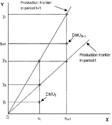
intuitive geometrical interpretation, and this can be exemplified in Figure 2.

[Figure 2]

In Figure 2, we can observe for the exemplified DMU that it produces less than

feasible under each period’s production frontier. The decomposition of the Malmquist

index according to equation (5) is given by the distance functions in equations (6) and

(7): p t r t y y y y E / / 1 +

= (6)

2 / 1 1 1 / / / /         × = + + q t p t r t q t y y y y y y y y

T . (7)

According to equations (6) and (7), efficiency change (E) is the ratio of the

(14)

and technical change (T) is the geometric mean of the shift in technology between

period t+1 and t.

3.2. Stochastic frontier

The DEA frontier is assumed to be deterministic, and differences between the

frontier and actual outputs are fully related to inefficiency. Suppose, alternatively to the

DEA approach, that the frontier is stochastic. In that case, such differences may also

stem from stochastic noise. Specifically, and after Battese and Coelli (1995) and Coelli

et al. (2002), assume the following model:

lny_it =F X( _it, )β η+ _it+ε_it (8)

it zit

η =θ (9)

where i is the country and t the time period. We have:

yit– the output, GDP per worker;

Xit – the vector of inputs, private and public capital per worker and human capital;

β – set of production function parameters to be estimated;

εi– normally distributed two-sided random error;

ηi– non-negative efficiency effect, assumed to have a truncated normal distribution;

zi – non-discretionary factors that explain inefficiency;

(15)

We have specified a log linear, Cobb-Douglas function for F(.). Within this setup, and

defining

2

2 2

η

η ε

σ γ

σ σ

=

+ , it is possible to produce a likelihood ratio statistic to test if γ=0,

i.e., that there are no random inefficiency effects.

Figure 3 illustrates the SFA production possibility frontier in the simple one

input-one output case.

[Figure 3]

4. Empirical analysis 4.1. Data

We use annual data for all inputs and outputs, for a set of OECD countries,

covering the period 1970-2000. Our output measure is GDP, measured in units of

national currency per PPS (purchasing power standard), per worker. As measures of

inputs we include public capital, private capital and human capital. The three measures

of capital are also scaled by worker (see the Appendix for further details and sources).5

Public capital was computed by using public capital to output ratios provided

by Kamps (2006). Private capital was obtained by subtracting public capital from total

capital. Human capital is the average years of schooling of the working age population.

Kaufmann, Kraay, and Mastruzzi (2008), based on hundreds of variables from

several sources, provide six indicators for six different dimensions of governance: voice

and accountability, political stability and absence of violence, government effectiveness,

regulatory quality, rule of law, and control of corruption. Therefore, we use such

5

(16)

composite indicator of government effectiveness (also disseminated by the World

Bank), as a non-discretionary factor.

4.2. Non-parametric analysis

We report in Table 1 the output-oriented variable returns to scale, technical

efficiency scores for each country, for the periods 1970, 1980, 1990 and 2000.6 From

Table 1 it is possible to observe that the number of countries that can be identified as

efficient was rather stable throughout time, with seven countries usually on the frontier

(Belgium, Canada, Spain, Italy, Japan, Portugal, and the USA), plus Norway in the last

period. Moreover, and apart from Canada in 2000, no other country shows up as

efficient by default, as can be seen by the listing of the respective peers, also reported in

Table 1.

[Table 1]

In addition, it is worthwhile noticing the steady improvement in technical

efficiency throughout the time sample for such countries as Ireland, Norway, and

Finland, with the first two countries reaching the efficiency frontier in 2000. An

opposite development can be seen for the case of Japan that shifts away from the

efficiency frontier between 1970 and 2000, and depicting the biggest TFP changes in

that period. Interestingly, Färe et al. (1994) who cover the period 1979-1988 for 17

OECD countries, report that the USA is the only country defining the efficiency

frontier, while Japan shows up as one of the least technically efficient countries in the

country sample, results that we also uncover in our broader sample.

6

(17)

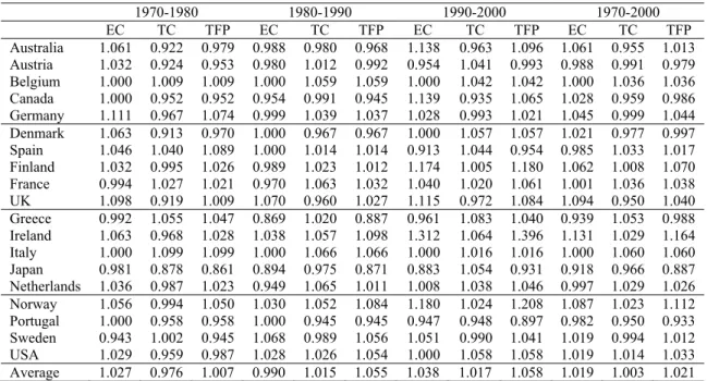
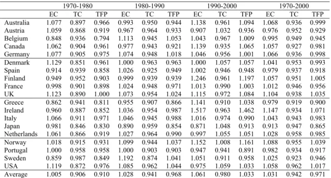
Table 2 reports the set of results for the Malmquist indices of efficiency,

technology and total factor productivity changes for the period 1970-2000, using GDP

per employee as the output measure and three inputs: private and public capital per

employee and human capital per employee. The results show that, on average for this

set of OECD countries, there was an improvement in total factor productivity (the

change was equal to 1.021). On the other hand, the close to unit average technology

change implies a small improvement in the underlying technology. Such marginal gains

in technology were additionally supported by the increase in efficiency (1.019), in order

to produce an increase in total factor productivity throughout the period. Interestingly,

the overall increase in total factor productivity in the period 1970-2000 occurred

essentially in the 1980s and in the 1990s.7

[Table 2]

The change in output can be decomposed into two components: the change in

total factor productivity and the quantitative change in the inputs, in other words,

Output TFP Input

∆ = ∆ × ∆ . (10)

Since we know the change in GDP and we can get the change in Total Factor

Productivity from the previous Malmquist set of results, the overall change in the inputs

can then be computed as∆Input= ∆Output/∆TFP. Therefore, we report in Table 3 the

7

(18)

changes in the overall input necessary to attain the output change, given the TFP

change.

[Table 3]

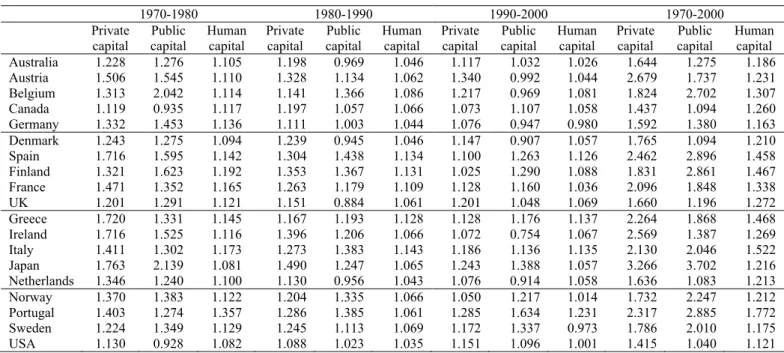
As a next step, we can also compute the period changes in each of the inputs that

we are considering, private capital, public capital and human capital. Table 4 reports

those changes. For instance, and for the sub-period 1970-1980, we can observe for

Australia overall period growth rates of 22.8%, 27.6%, and 10.5% respectively in

private capital, public capital and human capital.

[Table 4]

In addition, we can also decompose the increase in the inputs into those three

types of capital, imposing the restriction that the sum of the coefficients of the three

inputs equals unity.8 The specification is then

∆Input_i =a PrivK₁ _i+a PubK₂ _i+ − −(1 a₁ a HK₂) _i. (11)

where PrivK, PubK and HK are respectively private, public and human capital. The

regression results are shown in Table 5. It is interesting to observe that in the first

sub-period, input growth can be attributed to private capital and public capital by around

28% each, while human capital would account for the remaining 44%. However, in the

1980s and in the 1990s the contribution of private capital became more relevant, while

(19)

[Table 5]

We performed a sensitivity analysis with alternative specifications for the inputs

in the DEA and Malmquist efficiency computations. First, we included only private

capital and public capital as inputs; second we included total non-human capital, putting

together public and private capital, and human capital as the only two inputs (results are

reported in tables A1 to A4 in the Appendix).

Using a specification with only two inputs (private capital and public capital),

five countries are still on the frontier, Belgium, Canada, Spain, Portugal, and the USA

(as in the baseline specification), plus Norway in the last period and Japan in the first

period (as before), plus Denmark in the last three periods. Now, Italy is no longer in the

efficiency frontier. Not considering human capital as an input provides an average

increase in TFP only in the period 1990-2000 and decreases in the periods 1970-1980

and 1990-2000, which implies that human capital is a relevant input for the analysis. In

addition, for the entire time sample, positive efficiency gains are reported together with

losses stemming from the technology component of TFP.

Using a specification with two inputs (total non-human capital and human

capital) the number of countries on the frontier ranges from four countries (Belgium,

Italy, Portugal and the USA) in 1990 to seven countries in 2000 (Belgium, Denmark,

Ireland, Italy, Norway, Portugal and the USA). Regarding TFP, when considering total

non-human capital and human capital as inputs, it allows to uncover, for the entire

period, positive efficiency and technology gains and increases in TFP in all sub-periods.

8

(20)

4.3. Parametric analysis

Regarding our stochastic frontier analysis, we use the following baseline panel

data specification

0 1 2 3

lnGDP_it =β +β lnPrivK_it+β lnPubK_it +β HK_it+η_it+ε_it (12)

where i and t index respectively countries and time, GDP is GDP per employee, PrivK,

PubK and HK are respectively private, public and human capital per employee. In (12),

εit is a normally distributed random error, while ηit stands for a non-negative

inefficiency effect, assumed to have a truncated normal distribution. Inefficiency effects

can be explained by non-discretionary factors. In our case we assess whether the

exogenous factor wbg , which is an indicator of government effectiveness of the World

Bank, plays a role in explaining inefficiency scores.

The estimation of (12) produces estimates for the following parameters: the βs,

the coefficients associated to the inputs; θ, the constant associated to inefficiency; σε

and ση the standard deviations of respectively εit and

_

it

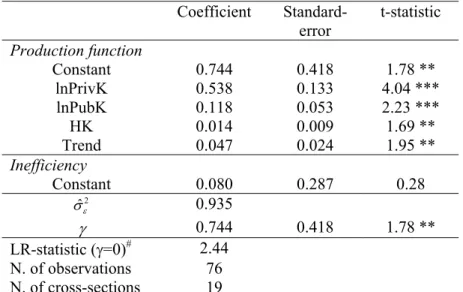
η . We report in Table 6 the

results for the stochastic frontier estimation, including also a time trend.9

[Table 6]

From Table 6 we observe that the inefficiency component of the model is not

statistically significant at the 10 percent level. Indeed, the LR statistic equals 2.44, and

9

(21)

the critical value at 10 percent for a mixed chi-square distribution with 2 degrees of

freedom is 3.808 (according to the tabulation of Kodde and Palm, 1986).

The coefficients for the three types of capital are all positive and statistically

significant. For instance, a one percent increase in private capital results in a 0.538

percent increase in output. In addition, a one percent increase in public and in human

capital leads respectively to a 0.118 and 0.014 percent increase in output.10

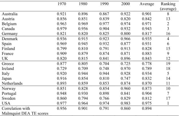
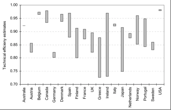
Table 7 reports the stochastic frontier estimates of technical efficiency, per year,

while Figure 4 illustrates the volatility of these efficiency measures. It is interesting to

observe the high correlations between the SFA technical efficiency estimates (Table 7)

and the DEA technical efficiency scores (Table 1) computed previously. Moreover, the

patterns already mentioned for such countries as Ireland, Finland and Norway (towards

the frontier) and Japan (away from the frontier) are also confirmed with the stochastic

analysis.

[Table 7]

[Figure 4]

In order to assess whether technical efficiency is related to better governance,

we use a composite indicator of government effectiveness of the World Bank (see

Kaufmann et al., 2008) and test its contribution to efficiency. The results in Table 8

show, for the period 1990-2000 (the government effectiveness indicator is an average

for the years 1996-2000), a positive effect of improved government effectiveness in

increasing technical efficiency and TFP, although not statistically significant in the

10

(22)

latter case. A positive effect from government effectiveness can also be found for the

SFA efficiency changes in the period 1990-2000.11

[Table 8]

5. Conclusion

In a cross section of OECD countries we replace the macroeconomic

production function by a production possibility frontier, TFP being the composite effect

of efficiency scores and possibility frontier changes. We consider, for the periods 1970,

1980, 1990, 2000, one output, GDP per worker, and three inputs, human capital, public

physical capital per worker and private physical per worker. We use a semi-parametric

analysis, computing Malmquist productivity indexes, and we also resort to stochastic

frontier analysis.

Our results show that: i) private capital is important for growth, and contributes

in a significant manner to output accumulation; ii) public and human capital

contributions are usually estimated as positive, but, depending on the specification, were

not always significant from a statistical point a view; iii) a governance indicator

(government effectiveness), a non-discretionary input, explains inefficiency. Indeed, our

results support the idea that better governance helps countries to achieve a better

performance and to operate closer to the production possibility frontier.

Deterministic and stochastic estimation methods provided similar results and

conclusions. Notably, non-parametric and parametric results coincide rather closely on

the countries movements vis-à-vis the possibility frontier and on their relative distances

to the frontier. The number of countries that can be nominated as efficient was rather

11

(23)

stable throughout the period, with six or seven countries usually on the frontier

(Belgium, Canada, Spain, Italy, Japan, Portugal, and the USA).

Our results have several policy implications. Our estimations imply that policy

may matter for growth by at least three different channels. One is public investment.

The public capital elasticity is imprecisely estimated. Our estimates and their variability

are consistent with other results concerning the effects of public investment across

countries. With other data and methods, we found that both patterns of crowding in

(public investment stimulating private investment and growth) and of crowding out are

to be found in the recent experience of industrialised countries.12 The policy content of

these results has to be seen with caution – macroeconomic analysis can be no substitute

for the careful evaluation of each public project on its own merits.

The second channel by which policy operates is governance. Our governance

indicator (government effectiveness) depends on policy in the broad sense of the word,

i.e., results not only from policy measures, but also from the way institutions are at the

same time shaped by history and designed by contemporaneous men and women.

Finally, our results are consistent with the importance of human capital

formation for growth. There is evidence of a positive macroeconomic return for human

capital investment, even if in the SFA specification the human capital coefficient does

not come out as statistically significant. Some countries in our sample, even if they are

close to or at the efficiency frontier (Portugal, Spain) are probably limited in their

growth prospects by their relative human capital scarcity.

Regarding future work developments, a possible step further could be the

computation of a parametric Malmquist index, using alternative approaches (e.g.

Fuentes et al., 2001, and Orea, 2004).

12

(24)

References

Acemoglu, D., Robinson, J. and Johnson, S. (2001). “The Colonial Origins of

Comparative Development: An Empirical Investigation”. American Economic

Review, 91 (5), 1369-1401.

Afonso, A. and St. Aubyn, M. (2006). "Cross-country Efficiency of Secondary

Education Provision: a Semi-parametric Analysis with Non-discretionary Inputs,"

Economic Modelling, 23 (3), 476-491.

Afonso, A. St. Aubyn, M. (2009). “Macroeconomic Rates of Return of Public and

Private Investment: Crowding-in and Crowding-out Effects”, Manchester School, 77

(S1), 21-39.

Afonso, A.; Schuknecht, L. and Tanzi, V. (2005). “Public Sector Efficiency: an

International Comparison,” Public Choice, 123 (3-4), 321-347.

Battese, G. and Coelli, T. (1995). “A Model for Technical Inefficiency Effects in a

Stochastic Frontier Production Function for Panel Data”, Empirical Economics, 20,

325-332.

Charnes, A.; Cooper, W. and Rhodes, E. (1978). “Measuring the efficiency of decision

making units”, European Journal of Operational Research, 2, 429–444.

Coelli T.; Rao, D. and Battese, G. (2002). An Introduction to Efficiency and

Productivity Analysis, 6th edition, Massachusetts, Kluwer Academic Publishers.

Cohen, D. and Soto, M. (2007). “Growth and human capital: good data, good results”,

Journal of Economic Growth, 12 (1), 51–76.

Delgado-Rodríguez, M. and Álvarez-Ayuso, I. (2008). “Economic Growth and

Convergence of EU Member States: An Empirical Investigation”, Review of

(25)

Färe, R.; Grosskopf, S.; Norris, M. and Zhang, Z. (1994). “Productivity Growth,

Technical Progress, and Efficiency Change in Industrialized Countries”, American

Economic Review, 84 (1), 66-83.

Färe, R.; Grosskopf, S. and Norris (1997). “Productivity Growth, Technical Progress,

and Efficiency Change in Industrialized Countries: Reply”, American Economic

Review, 87 (5), 1040-1044.

Farrell, M. (1957). “The Measurement of Productive Efficiency”, Journal of the Royal

Statistical Society Series A (General), 120, 253-281.

Fuentes, H., Grifell-Tatjé, E. and Perelman, S. (2001), “A Parametric Distance Function

Approach for Malmquist Productivity Index Estimation”, Journal of Productivity

Analysis, 15, 79-94.

Hendersen, D. and Russel, R. (2005). “Human capital and convergence: a

production-frontier approach”, International Economic Review, 46 (4), 1167-1205.

Jerzmanowski, M. (2007). "Total factor productivity differences: Appropriate

technology vs. efficiency," European Economic Review, 51 (8), 2080-2110.

Kamps, C. (2006). “New Estimates of Government Net Capital Stocks for 22 OECD

Countries, 1960–2001,” IMF Staff Papers, 53 (1), 120-150.

Kaufmann, D., Kraay, A. and Mastruzzi, M. (2008). “Governance Matters VII:

Aggregate and Individual Governance Indicators for 1996–2007”, World Bank

Policy Research Working Paper 4654.

Kodde, D. and Palm, F. (1986). “Wald Criteria for Jointly Testing Equality and

Inequality Restrictions”, Econometrica, 54 (5), 1243-1248.

Koop, G.; Osiewalski, J. and Steel, M. (2000). “A stochastic frontier analysis of output

level and growth in Poland and western economies”. Economics of Planning, 33(3),

(26)

Krüger (2003). “The global trends of total factor productivity: evidence from the

nonparametric Malmquist index approach”, Oxford Economic Papers, 55, 265-286.

Kumar, S. and Russell, R. (2002). “Technological Change, Technological Catch-up, and

Capital Deepening: Relative Contributions to Growth and Convergence”, American

Economic Review, 92 (3), 527-548.

Malmquist, S. (1953). “Index Numbers and Indifference Surfaces”, Trabajos de

Estadística, 4, 209-242.

Mastromacro, C. and Ghosh, S. (20008). “Foreign Capital, Human Capital, and

Efficiency: A Stochastic Frontier Analysis for Developing Countries”, World

Development, forthcoming.

Olson Jr., M., Sarna, N. and Swamy, A. (2000). “Governance and growth: A simple

hypothesis explaining cross-country differences in productivity growth”, Public

Choice, 102 (3-4), 341-364.

Orea, L. (2002). “Parametric Decomposition of a Generalized Malmquist Productivity

Index”, Journal of Productivity Analysis, 18, 5-22.

Ray, S and Desli, E. (1997). “Productivity Growth, Technical Progress, and Efficiency

Change in Industrialized Countries: Comment”, American Economic Review, 87 (5),

1033-1039.

Thanassoulis, E. (2001). Introduction to the Theory and Application of Data

(27)

Appendix – Data sources

Original series Ameco codes

Gross Domestic Product at 2000 prices, thousands national currency 1/ 1.1.0.0.OVGD

Net capital stock at 2000 prices: total economy 1/ 1.0.0.0.OKND

Employment, persons: all domestic industries (National accounts) 1/ 1.0.0.0.NETD GDP purchasing power parities, Units of national currency per PPS

(purchasing power standard) 1/ 1.0.212.0.KPN

Human capital (average years of schooling of the working age population) 2/

Government net capital stock, volume 3/

Private total net capital stock, volume Our computation

Government effectiveness 4/

1/ Series from the European Commission AMECO database. 2/ Cohen and Soto (2007).

3/ Kamps (2006).

(28)

Table 1 – Output-oriented DEA VRS technical efficiency scores

(output: GDP per employee; inputs: private and public capital, human capital)

1970 Peers 1980 Peers 1990 Peers 2000 Peers

Australia 0.932 FI, CA, NL _0.937 CA, US, PR _0.924 CA, BE, PT _0.970 DK, IR, PT Austria 0.897 CA, US, JP, PT _0.905 DK, US, PT _0.854 US, BE, PT _0.817 US, IT, BE

Belgium 1.000 BE _1.000 BE _1.000 BE _1.000 BE

Canada 1.000 CA _1.000 CA _1.000 CA _1.000 CA

Germany 0.846 BE, CA _0.906 BE, PT _0.891 IT, BE _0.814 DK, BE, US Denmark 0.999 US, NL, PT _1.000 DK _1.000 DK _1.000 DK Spain 1.000 ES _1.000 ES _1.000 ES _0.943 IT, PT, IR Finland 0.812 ES, BE, CA _0.852 ES, BE, PT _0.864 BE, CA, ES _0.915 BE, US, IR France 0.942 ES. US, IT, CA _0.935 US, IT _0.941 IT, US _0.920 NO, IT, US UK 0.825 US, IT, ES, PT _0.858 PT, US, DK _0.898 BE, US, PT _0.968 DK, IR, PT Greece 0.915 US, IT, ES, PT _0.884 BE, ES, IT _0.782 ES, CA, PT _0.749 PT, IR, IT Ireland 0.744 US, CA, JP, PT _0.737 US, BE, PT _0.765 BE, US, IT _1.000 IR

Italy 1.000 IT _1.000 IT _1.000 IT _1.000 IT

Japan 1.000 JP _0.984 DK, PT _0.877 DK, US, PT _0.775 US, DK Netherlands 0.912 US, IT, PR _0.919 BE, US, IT _0.869 US, IT, BE _0.871 IR, US, PT Norway 0.882 BE, CA _0.917 BE. US _0.955 IT, US _1.000 NO

Portugal 1.000 PR _1.000 PT _1.000 PT _1.000 PT

Sweden 0.929 BE, CA _0.900 BE, ES _0.975 CA, PT _0.881 BE, IR

USA 1.000 US _1.000 US _1.000 US _1.000 US

Average 0.928 0.933 0.926 0.928

Countries on the

frontier 7 7 7 8

Note: VRS – variable returns to scale.

Table 2 – Malmquist efficiency, technology, and total factor productivity change indices (Output-oriented): 1970-2000 (output; GDP; inputs: private and public capital, human

capital)

1970-1980 1980-1990 1990-2000 1970-2000 EC TC TFP EC TC TFP EC TC TFP EC TC TFP Australia 1.061 0.922 0.979 0.988 0.980 0.968 1.138 0.963 1.096 1.061 0.955 1.013

Austria 1.032 0.924 0.953 0.980 1.012 0.992 0.954 1.041 0.993 0.988 0.991 0.979

Belgium 1.000 1.009 1.009 1.000 1.059 1.059 1.000 1.042 1.042 1.000 1.036 1.036

Canada 1.000 0.952 0.952 0.954 0.991 0.945 1.139 0.935 1.065 1.028 0.959 0.986

Germany 1.111 0.967 1.074 0.999 1.039 1.037 1.028 0.993 1.021 1.045 0.999 1.044

Denmark 1.063 0.913 0.970 1.000 0.967 0.967 1.000 1.057 1.057 1.021 0.977 0.997

Spain 1.046 1.040 1.089 1.000 1.014 1.014 0.913 1.044 0.954 0.985 1.033 1.017

Finland 1.032 0.995 1.026 0.989 1.023 1.012 1.174 1.005 1.180 1.062 1.008 1.070

France 0.994 1.027 1.021 0.970 1.063 1.032 1.040 1.020 1.061 1.001 1.036 1.038

UK 1.098 0.919 1.009 1.070 0.960 1.027 1.115 0.972 1.084 1.094 0.950 1.040

Greece 0.992 1.055 1.047 0.869 1.020 0.887 0.961 1.083 1.040 0.939 1.053 0.988

Ireland 1.063 0.968 1.028 1.038 1.057 1.098 1.312 1.064 1.396 1.131 1.029 1.164

Italy 1.000 1.099 1.099 1.000 1.066 1.066 1.000 1.016 1.016 1.000 1.060 1.060

Japan 0.981 0.878 0.861 0.894 0.975 0.871 0.883 1.054 0.931 0.918 0.966 0.887

Netherlands 1.036 0.987 1.023 0.949 1.065 1.011 1.008 1.038 1.046 0.997 1.029 1.026

Norway 1.056 0.994 1.050 1.030 1.052 1.084 1.180 1.024 1.208 1.087 1.023 1.112

Portugal 1.000 0.958 0.958 1.000 0.945 0.945 0.947 0.948 0.897 0.982 0.950 0.933

Sweden 0.943 1.002 0.945 1.068 0.989 1.056 1.051 0.990 1.041 1.019 0.994 1.012

USA 1.029 0.959 0.987 1.028 1.026 1.054 1.000 1.058 1.058 1.019 1.014 1.033

Average 1.027 0.976 1.007 0.990 1.015 1.055 1.038 1.017 1.058 1.019 1.003 1.021

(29)

Table 3 – Output, input and TFP variations (index changes)

1970-1980 1980-1990 1990-2000 1970-2000

∆GDP ∆TFP ∆Input ∆GDP ∆TFP ∆Input ∆GDP ∆TFP ∆Input ∆GDP ∆TFP ∆Input

Australia 1.189 0.922 1.215 1.121 0.968 1.158 1.199 1.096 1.094 1.598 1.013 1.578

Austria 1.387 0.924 1.456 1.233 0.992 1.243 1.205 0.993 1.214 2.061 0.979 2.106

Belgium 1.356 1.009 1.344 1.209 1.059 1.141 1.163 1.042 1.116 1.906 1.036 1.839

Canada 1.065 0.952 1.118 1.098 0.945 1.162 1.151 1.065 1.081 1.346 0.986 1.365

Germany 1.304 0.967 1.215 1.127 1.037 1.087 1.045 1.021 1.024 1.536 1.044 1.471

Denmark 1.198 0.913 1.235 1.189 0.967 1.229 1.202 1.057 1.137 1.710 0.997 1.715

Spain 1.440 1.040 1.322 1.259 1.014 1.242 1.077 0.954 1.128 1.951 1.017 1.919

Finland 1.337 0.995 1.303 1.271 1.012 1.256 1.295 1.180 1.098 2.200 1.070 2.056

France 1.315 1.027 1.288 1.223 1.032 1.185 1.139 1.061 1.074 1.833 1.038 1.766

UK 1.207 0.919 1.196 1.166 1.027 1.135 1.260 1.084 1.162 1.771 1.040 1.703

Greece 1.345 1.055 1.284 1.023 0.887 1.153 1.196 1.040 1.150 1.645 0.988 1.665

Ireland 1.451 0.968 1.412 1.370 1.098 1.248 1.434 1.396 1.027 2.850 1.164 2.448

Italy 1.365 1.099 1.242 1.262 1.066 1.184 1.162 1.016 1.144 2.003 1.060 1.889

Japan 1.462 0.878 1.698 1.273 0.871 1.462 1.135 0.931 1.219 2.113 0.887 2.382

Netherlands 1.228 0.987 1.201 1.112 1.011 1.100 1.118 1.046 1.069 1.527 1.026 1.488

Norway 1.277 0.994 1.216 1.253 1.084 1.156 1.266 1.208 1.048 2.025 1.112 1.821

Portugal 1.289 0.958 1.346 1.206 0.945 1.277 1.209 0.897 1.348 1.880 0.933 2.016

Sweden 1.131 1.002 1.197 1.164 1.056 1.102 1.281 1.041 1.230 1.687 1.012 1.667

USA 1.087 0.959 1.101 1.133 1.054 1.075 1.187 1.058 1.122 1.461 1.033 1.414

Note: ∆Input=∆GDP/∆TFP.

Table 4 – Input variations (index changes)

1970-1980 1980-1990 1990-2000 1970-2000

Private capital Public capital Human capital Private capital Public capital Human capital Private capital Public capital Human capital Private capital Public capital Human capital

Australia 1.228 1.276 1.105 1.198 0.969 1.046 1.117 1.032 1.026 1.644 1.275 1.186

Austria 1.506 1.545 1.110 1.328 1.134 1.062 1.340 0.992 1.044 2.679 1.737 1.231

Belgium 1.313 2.042 1.114 1.141 1.366 1.086 1.217 0.969 1.081 1.824 2.702 1.307

Canada 1.119 0.935 1.117 1.197 1.057 1.066 1.073 1.107 1.058 1.437 1.094 1.260

Germany 1.332 1.453 1.136 1.111 1.003 1.044 1.076 0.947 0.980 1.592 1.380 1.163

Denmark 1.243 1.275 1.094 1.239 0.945 1.046 1.147 0.907 1.057 1.765 1.094 1.210

Spain 1.716 1.595 1.142 1.304 1.438 1.134 1.100 1.263 1.126 2.462 2.896 1.458

Finland 1.321 1.623 1.192 1.353 1.367 1.131 1.025 1.290 1.088 1.831 2.861 1.467

France 1.471 1.352 1.165 1.263 1.179 1.109 1.128 1.160 1.036 2.096 1.848 1.338

UK 1.201 1.291 1.121 1.151 0.884 1.061 1.201 1.048 1.069 1.660 1.196 1.272

Greece 1.720 1.331 1.145 1.167 1.193 1.128 1.128 1.176 1.137 2.264 1.868 1.468

Ireland 1.716 1.525 1.116 1.396 1.206 1.066 1.072 0.754 1.067 2.569 1.387 1.269

Italy 1.411 1.302 1.173 1.273 1.383 1.143 1.186 1.136 1.135 2.130 2.046 1.522

Japan 1.763 2.139 1.081 1.490 1.247 1.065 1.243 1.388 1.057 3.266 3.702 1.216

Netherlands 1.346 1.240 1.100 1.130 0.956 1.043 1.076 0.914 1.058 1.636 1.083 1.213

Norway 1.370 1.383 1.122 1.204 1.335 1.066 1.050 1.217 1.014 1.732 2.247 1.212

Portugal 1.403 1.274 1.357 1.286 1.385 1.061 1.285 1.634 1.231 2.317 2.885 1.772

Sweden 1.224 1.349 1.129 1.245 1.113 1.069 1.172 1.337 0.973 1.786 2.010 1.175

(30)

Table 5 – Decomposition of the change in total input

Private capital

(α1)

Public capital (α2)

Human capital (1-α1-α2)

R-square N 1970-1980 0.277 ***

(3.63)

0.276 *** (4.50)

0.446 # 0.77 19

1980-1990 0.733 *** (11.65)

-0.025 (-0.37)

0.293 # 0.79 19

1990-2000 0.652 *** (11.82)

0.183 *** (5.36)

0.165 # 0.89 19

1970-2000 0.556 *** (6.93)

0.116 (1.61)

0.328 # 0.80 19

Note: t-statistics in brackets.

*, ** and *** denote level of significance indicating 10%, 5% and 1% respectively.

#

,Wald test rejects the null (1-α1-α2)=0 at the 1% level of significance.

Table 6 – Stochastic frontier estimation results (with time trend)

Coefficient

Standard-error

t-statistic

Production function

Constant 0.744 0.418 1.78 **

lnPrivK 0.538 0.133 4.04 ***

lnPubK 0.118 0.053 2.23 ***

HK 0.014 0.009 1.69 **

Trend 0.047 0.024 1.95 **

Inefficiency

Constant 0.080 0.287 0.28

2

ˆ_ε

σ 0.935

γ 0.744 0.418 1.78 **

LR-statistic (γ=0)# 2.44

N. of observations 76

N. of cross-sections 19

(31)

Table 7 – SFA efficiency scores (with time trend)

1970 1980 1990 2000 Average Ranking (average)

Australia 0.921 0.896 0.867 0.922 0.901 8

Austria 0.856 0.851 0.839 0.820 0.842 13

Belgium 0.963 0.969 0.977 0.974 0.971 2

Canada 0.979 0.956 0.904 0.932 0.943 3

Germany 0.821 0.820 0.825 0.800 0.817 16

Denmark 0.936 0.915 0.923 0.966 0.935 4

Spain 0.969 0.945 0.932 0.877 0.931 6

Finland 0.799 0.810 0.791 0.913 0.828 15

France 0.909 0.879 0.874 0.871 0.883 9

UK 0.820 0.815 0.841 0.896 0.843 12

Greece 0.877 0.805 0.704 0.725 0.778 19

Ireland 0.729 0.709 0.748 0.970 0.789 18

Italy 0.920 0.944 0.944 0.928 0.934 5

Japan 0.916 0.854 0.810 0.747 0.832 14

Netherlands 0.893 0.859 0.853 0.874 0.870 11

Norway 0.851 0.828 0.854 0.960 0.873 10

Portugal 0.948 0.930 0.898 0.841 0.904 7

Sweden 0.860 0.794 0.766 0.829 0.812 17

USA 0.977 0.964 0.974 0.983 0.975 1

Correlation with

Malmquist DEA TE scores

0.956 0.901 0.791 0.860 0.894

Table 8 – Efficiency and government effectiveness (1990-2000)

Dependent variable

Constant Government effectiveness

R-square N Technical

efficiency change

0.844 *** (8.35)

0.112 ** (2.04)

0.20 19 TFP change 0.891 ***

(8.37)

0.100 (1.65)

0.14 19 SFA efficiency

change

0.095 (1.42)

0.071 * (1.87)

0.17 19

Note: t-statistics in brackets.

(32)

Figure 1 – DEA production possibility frontier

(33)

Figure 3 – SFA production possibility frontier

Figure 4 – SFA efficiency scores, with time trend (1970, 1980, 1990, 2000)

0.70 0.75 0.80 0.85 0.90 0.95 1.00 A u s tr a lia Au s tr ia B e lg iu m C anada G er m any De n m a rk S pai n F inl and F ranc e UK G reec e Ir el

and Ital

(34)

Annex – Additional estimates

Table A1 – Output-oriented DEA VRS technical efficiency scores (output: GDP per employee; inputs: private and public capital)

1970 1980 1990 2000

Australia 0.932 0.937 0.924 0.970

Austria 0.886 0.890 0.832 0.806

Belgium 1.000 1.000 1.000 1.000

Canada 1.000 1.000 1.000 1.000

Germany 0.846 0.906 0.891 0.814

Denmark 0.989 1.000 1.000 1.000

Spain 1.000 1.000 0.995 0.851

Finland 0.812 0.852 0.862 0.915

France 0.878 0.907 0.941 0.896

UK 0.825 0.858 0.898 0.968

Greece 0.862 0.860 0.772 0.710

Ireland 0.732 0.694 0.759 1.000

Italy 0.884 0.961 1.000 0.976

Japan 1.000 0.984 0.877 0.775

Netherlands 0.877 0.873 0.857 0.837

Norway 0.882 0.917 0.955 1.000

Portugal 1.000 1.000 1.000 1.000

Sweden 0.929 0.900 0.975 0.881

USA 1.000 1.000 1.000 1.000

Average 0.912 0.923 0.923 0.916

Countries on the frontier 6 6 6 7

Table A2 – Malmquist efficiency, technology, and total factor productivity change indices (Output-oriented: 1970-2000; output; GDP; inputs: private and public capital)

1970-1980 1980-1990 1990-2000 1970-2000

EC TC TFP EC TC TFP EC TC TFP EC TC TFP Australia 1.077 0.897 0.966 0.993 0.950 0.944 1.138 0.961 1.094 1.068 0.936 0.999

Austria 1.059 0.868 0.919 0.967 0.964 0.933 0.907 1.032 0.936 0.976 0.952 0.929

Belgium 0.848 0.936 0.794 1.113 0.945 1.053 1.043 0.967 1.009 0.995 0.949 0.945

Canada 1.062 0.904 0.961 0.977 0.943 0.921 1.139 0.935 1.065 1.057 0.927 0.981

Germany 1.077 0.905 0.975 1.074 0.948 1.018 1.046 0.956 1.001 1.066 0.936 0.998

Denmark 1.129 0.851 0.961 1.000 0.963 0.963 1.000 1.057 1.057 1.041 0.953 0.993

Spain 0.914 0.939 0.858 1.026 0.925 0.949 1.002 0.946 0.948 0.979 0.937 0.918

Finland 0.949 0.952 0.903 0.999 0.939 0.939 1.246 0.961 1.197 1.057 0.951 1.005

France 0.998 0.901 0.898 1.024 0.948 0.971 1.013 0.990 1.003 1.012 0.946 0.956

UK 1.123 0.890 1.000 1.073 0.954 1.024 1.115 0.972 1.084 1.104 0.938 1.035

Greece 0.862 0.941 0.811 0.955 0.907 0.866 1.141 0.910 1.038 0.979 0.919 0.900

Ireland 0.960 0.887 0.852 1.036 0.954 0.987 1.517 0.963 1.462 1.147 0.934 1.071

Italy 1.066 0.911 0.971 1.046 0.945 0.988 1.016 0.974 0.990 1.043 0.943 0.983

Japan 0.981 0.846 0.830 0.890 0.959 0.854 0.871 1.048 0.913 0.913 0.947 0.865

Netherlands 1.061 0.866 0.919 1.027 0.964 0.990 0.997 1.055 1.051 1.028 0.958 0.985

Norway 1.018 0.915 0.931 1.099 0.944 1.037 1.152 1.008 1.161 1.088 0.955 1.039

Portugal 1.000 0.958 0.958 1.000 0.903 0.903 0.947 0.941 0.891 0.982 0.934 0.917

Sweden 0.859 0.987 0.849 1.192 0.874 1.041 1.051 0.911 0.958 1.025 0.923 0.946

USA 1.119 0.872 0.976 1.085 0.962 1.044 0.975 1.059 1.033 1.058 0.962 1.017

Average 1.005 0.906 0.910 1.028 0.941 0.968 1.061 0.980 1.033 1.031 0.942 0.971

(35)

Table A3 – Output-oriented DEA VRS technical efficiency scores (output: GDP per employee; inputs: total capital and human capital)

1970 1980 1990 2000

Australia 0.931 0.930 0.884 0.914

Austria 0.870 0.864 0.828 0.815

Belgium 0.977 1.000 1.000 1.000

Canada 1.000 1.000 0.919 0.930

Germany 0.808 0.877 0.873 0.768

Denmark 0.947 0.945 0.966 1.000

Spain 1.000 1.000 0.990 0.940

Finland 0.786 0.828 0.777 0.901

France 0.941 0.935 0.940 0.919

UK 0.816 0.843 0.882 0.899

Greece 0.914 0.856 0.725 0.745

Ireland 0.724 0.721 0.764 1.000

Italy 1.000 1.000 1.000 1.000

Japan 1.000 0.863 0.784 0.711

Netherlands 0.895 0.919 0.864 0.859

Norway 0.828 0.872 0.949 1.000

Portugal 1.000 1.000 1.000 1.000

Sweden 0.834 0.799 0.769 0.836

USA 1.000 1.000 1.000 1.000

Average 0.909 0.908 0.890 0.907

Countries on the frontier 6 6 4 7

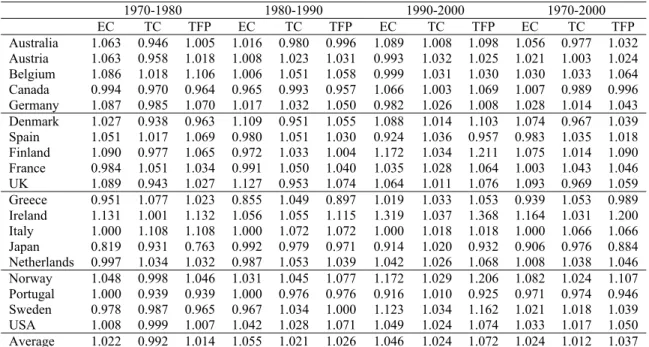
Table A4 – Malmquist efficiency, technology, and total factor productivity change indices (Output-oriented: 1970-2000; output; GDP; inputs: total capital and human

capital)

1970-1980 1980-1990 1990-2000 1970-2000

EC TC TFP EC TC TFP EC TC TFP EC TC TFP Australia 1.063 0.946 1.005 1.016 0.980 0.996 1.089 1.008 1.098 1.056 0.977 1.032

Austria 1.063 0.958 1.018 1.008 1.023 1.031 0.993 1.032 1.025 1.021 1.003 1.024

Belgium 1.086 1.018 1.106 1.006 1.051 1.058 0.999 1.031 1.030 1.030 1.033 1.064

Canada 0.994 0.970 0.964 0.965 0.993 0.957 1.066 1.003 1.069 1.007 0.989 0.996

Germany 1.087 0.985 1.070 1.017 1.032 1.050 0.982 1.026 1.008 1.028 1.014 1.043

Denmark 1.027 0.938 0.963 1.109 0.951 1.055 1.088 1.014 1.103 1.074 0.967 1.039

Spain 1.051 1.017 1.069 0.980 1.051 1.030 0.924 1.036 0.957 0.983 1.035 1.018

Finland 1.090 0.977 1.065 0.972 1.033 1.004 1.172 1.034 1.211 1.075 1.014 1.090

France 0.984 1.051 1.034 0.991 1.050 1.040 1.035 1.028 1.064 1.003 1.043 1.046

UK 1.089 0.943 1.027 1.127 0.953 1.074 1.064 1.011 1.076 1.093 0.969 1.059

Greece 0.951 1.077 1.023 0.855 1.049 0.897 1.019 1.033 1.053 0.939 1.053 0.989

Ireland 1.131 1.001 1.132 1.056 1.055 1.115 1.319 1.037 1.368 1.164 1.031 1.200

Italy 1.000 1.108 1.108 1.000 1.072 1.072 1.000 1.018 1.018 1.000 1.066 1.066

Japan 0.819 0.931 0.763 0.992 0.979 0.971 0.914 1.020 0.932 0.906 0.976 0.884

Netherlands 0.997 1.034 1.032 0.987 1.053 1.039 1.042 1.026 1.068 1.008 1.038 1.046

Norway 1.048 0.998 1.046 1.031 1.045 1.077 1.172 1.029 1.206 1.082 1.024 1.107

Portugal 1.000 0.939 0.939 1.000 0.976 0.976 0.916 1.010 0.925 0.971 0.974 0.946

Sweden 0.978 0.987 0.965 0.967 1.034 1.000 1.123 1.034 1.162 1.021 1.018 1.039

USA 1.008 0.999 1.007 1.042 1.028 1.071 1.049 1.024 1.074 1.033 1.017 1.050

Average 1.022 0.992 1.014 1.055 1.021 1.026 1.046 1.024 1.072 1.024 1.012 1.037

(36)

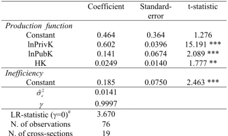
Table A5 – Stochastic frontier estimation results (without time trend)

Coefficient

Standard-error

t-statistic

Production function

Constant 0.464 0.364 1.276

lnPrivK 0.602 0.0396 15.191 ***

lnPubK 0.141 0.0674 2.089 ***

HK 0.0249 0.0140 1.777 **

Inefficiency

Constant 0.185 0.0750 2.463 ***

2

ˆ_ε

σ 0.0141

γ 0.9997

LR-statistic (γ=0)# 3.670

N. of observations 76 N. of cross-sections 19

# The LR statistic critical value at 10% for a mixed chi-square distribution with 2 degrees of freedom is 3.808, according to the tabulation of Kodde and Palm (1986). *, ** and *** denote level of significance indicating 10%, 5% and 1% respectively.

Table A6 – SFA efficiency scores (without time trend)

1970 1980 1990 2000 Average Ranking (average)

Australia 0.816 0.804 0.801 0.887 0.827 8

Austria 0.785 0.780 0.784 0.784 0.783 12

Belgium 0.903 0.918 0.961 0.977 0.940 2

Canada 0.902 0.879 0.843 0.901 0.881 7

Germany 0.713 0.715 0.745 0.756 0.732 19

Denmark 0.852 0.845 0.878 0.969 0.886 5

Spain 0.956 0.910 0.905 0.867 0.910 4

Finland 0.740 0.753 0.740 0.889 0.780 13

France 0.829 0.802 0.811 0.834 0.819 9

UK 0.729 0.736 0.788 0.865 0.779 14