An extensible toolbox for modeling nature
e
society interactions
Tiago Garcia de Senna Carneiro
a,*, Pedro Ribeiro de Andrade
b, Gilberto Câmara
c,
Antônio Miguel Vieira Monteiro
c, Rodrigo Reis Pereira
aaEarth System Simulation Laboratory (TerraLAB), Federal University of Ouro Preto (UFOP), Campus Universitário, Morro do Cruzeiro, Ouro Preto, MG 35900-000, Brazil
bEarth System Science Center (CCST), National Institute for Space Research (INPE), Av. dos Astronautas 1758, São José dos Campos, SP 12227-001, Brazil cImage Processing Division (DPI), National Institute for Space Research (INPE), Av. dos Astronautas 1758, São José dos Campos, SP 12227-001, Brazil
a r t i c l e
i n f o
Article history: Received 21 March 2012 Received in revised form 8 February 2013 Accepted 7 March 2013 Available online 12 April 2013
Keywords:
Natureesociety models
Multi-scale modeling Environmental modeling Discrete event simulation Cellular automata Multi-agent systems
a b s t r a c t
Modeling interactions between social and natural systems is a hard task. It involves collecting data, building up a conceptual approach, implementing, calibrating, simulating, validating, and possibly repeating these steps again and again. There are different conceptual approaches proposed in the literature to tackle this problem. However, for complex problems it is better to combine different ap-proaches, giving rise to a need forflexible and extensible frameworks for modeling natureesociety
in-teractions. In this paper we present TerraME, an open source toolbox that supports multi-paradigm and multi-scale modeling of coupled human-environmental systems. It enables models that combine agent-based, cellular automata, system dynamics, and discrete event simulation paradigms. TerraME has a GIS interface for managing real-world geospatial data and uses Lua, an expressive scripting language.
Ó2013 Elsevier Ltd. All rights reserved.
1. Introduction
Planners and policy makers need models that capture how human actions act on natural systems (Turner et al., 1995). These
models represent coupled natureesociety systems in different ways. Their capacity to capture the impact of human actions in nature depends on the spatial and temporal scales used. It also hinges on the chosen hypotheses about human behavior and environmental response. Despite the challenges involved in building them, these models have an important role. They bring forth unstated assumptions hidden in policy proposals, helping us to understand the possible results of different choices (Moran, 2010).
In this paper, we use the termparadigmto mean a worldview intrinsic to a scientific theory. Models of natureesociety in-teractions use different paradigms, including cellular automata, agent-based models, map algebra, and system dynamics (White and Engelen, 1997;Parker et al., 2003;Karssenberg and De Jong, 2005;Batty, 2012). In many cases using a single paradigm is not enough. For complex problems, it is better to combine different methods to learn more about how human societies interact with nature (Rindfuss et al., 2004).
Most designers of natureesociety modeling tools choose a paradigm and build a toolbox that supports it. Supporting a single paradigm has many advantages. Most paradigms have a lot of documentation and user communities, which helps potential adopters. However, designer choices may also limit a software’s Software availability
Name: TerraME
Developer: Federal University of Ouro Preto (UFOP), Brazil; National Institute for Space Research (INPE), Brazil
Contact:[email protected],[email protected] Programming language: Lua
Optional additional software: MySQL and TerraView License: GNU LGPL (open source)
Website:http://www.terrame.org
*Corresponding author. Tel.:þ55 (31) 3559 1692; fax:þ55 (31) 3559 1660. E-mail addresses:[email protected] (T.G.S. Carneiro),[email protected] (P.R. Andrade), [email protected] (G. Câmara), [email protected] (A.M.V. Monteiro),[email protected](R.R. Pereira).
Contents lists available atSciVerse ScienceDirect
Environmental Modelling & Software
j o u r n a l h o m e p a g e : w w w . e l s e v i e r . c o m / l o c a t e / e n v s o f t
e ”
lows, we refer to this challenge as themulti-paradigm model design problem.
This paper presents a possible response to this question. We were inspired by how Bjarne Stroustrup built Cþþ(Stroustrup, 1994). He designed Cþþin a bottom-up, modular fashion, allow-ing object-oriented, generic programmallow-ing, and procedural pro-gramming styles. Theflexibility of Cþþhas no doubt contributed to its widespread use. Following these ideas, our proposed solution for the multi-paradigm model design problem stems from three conjectures. First, the tool should provide acollection of data types and functions needed by different paradigms. This leads to a bottom-up design based on building blocks that are combined by the modeller. The second conjecture is that natureesociety in-teractions happen in geographical space. Unlike human and capital resources, that are mobile, natural resources are fixed. When dealing with environmental problems, we have to capture geographical features such as soil, climate, vegetation, and biodi-versity in a spatially explicit way. Thus, models for natureesociety interactions need a spatial component that represents natural landscapes and the results of human interactions with them. Third,
natureesociety interactions occur at different scales. Many problems need to be expressed as multi-scale models where matter, energy, and informationflow between different scales. The toolkit should allow the user to break a complex model into simpler sub-models. Each sub-model is a micro-world with its own temporal and spatial resolution and behavior. Sub-models can then be nested and combined in different ways. Thus, our proposed architecture puts together aset of data typeswithmethods to build and connect geospatial micro-worlds.
Based on these conjectures, we have designed and implemented the TerraME toolbox. It has building blocks for model development, allowing the user to specify the spatial, temporal, and behavioral parts of a model independently. Its components are expressive, enabling different approaches to be combined. TerraME’s main aim isflexibility. It does not enforce a unique modeling paradigm, but provides the tools needed by the modeller. TerraME is an open source software distributed under the GNU LGPL license and is available atwww.terrame.org.
In the next section, we consider the challenges for designing software to model natureesociety interactions, pointing out the choices we made. We describe the general architecture of TerraME in Section3. Section4has examples that show the main features of TerraME. Wefinish the paper by reflecting on the contributions and the limits of our proposed solution to the multi-paradigm model design problem.
2. Design choices for natureesociety interaction modeling toolboxes
In this section, we discuss four decisions faced by designers of modeling tools that support natureesociety interactions. In each case, we point out the choices we made in TerraME.
Choosing which modeling paradigms to support.
Selecting the model interface.
Defining how the model interfaces with databases and GIS.
Providing tools for verification, calibration, and validation.
complex patterns from simple rules. In the system dynamics view, the world consists of stocks of energy, information, or matter. Model rules are differential equations definingflows that transport energy, information or matter between stocks. Agent-based models represent autonomous individuals that interact with themselves, the environment, and other agents. Map algebra uses raster maps to allocate properties in space and provides functions over maps to convey change. In the discrete event formalism, an event is an in-dividual temporal episode. Instead of having functions that compute the next step of the simulation, an event-based model has a set of events and conditions when they occur.
Most existing modeling tools are centered on a paradigm, although they may support others. Examples of agent-based modeling tools are NetLogo (Tisue and Wilensky, 2004) and RePast (North et al., 2006). System modeling tools include STELLA (Roberts et al., 1983), Vensim (Eberlein and Peterson, 1992), and Simile (Muetzelfeldt and Massheder, 2003). PCRaster is a map algebra toolbox with extensions for dynamic modeling (Karssenberg et al., 2001,2009;Wesseling et al., 1996). JDEVS is an event-based modeling software (Filippi and Bisgambiglia, 2004). Focusing in a paradigm favors knowledge reuse. Users familiar with one modeling paradigm will be comfortable when facing a new toolbox based on similar ideas. If one knows STELLA, learning Vensim and Simile is straightforward. Models developed in Net-Logo can be ported to RePast without excessive work (Crooks and Castle, 2012). Designers can also extend an existing tool to sup-port other paradigms than their original choice.
The alternative is to build a multi-paradigm modeling tool in a bottom-up way. This is what we did in TerraME since we hold that natureesociety relations are inherently complex. As expressed by Mike Batty:“in modeling, the quest for parsimony, simplicity, and homogeneity is increasingly being confronted by the need for plausibility, richness, and heterogeneity” (Batty, 2012). A multi-paradigm toolbox allows modellers to combine different para-digms when solving a problem. However, such tools are harder to learn since there are many concepts to be grasped. Flexibility comes at a price. We recognize that not all users will be willing to make it, although we believe the effort is worthwhile.
2.2. Selecting the model interface
Modeling toolboxes need to provide analytical power to ex-press complex problems. Nearly all tools use a programming lan-guage with additional high-level statements. Some tools also provide icon-based graphical programming, like the system dy-namicstools STELLA and Simile. Visual interfaces are appealing and enable decision-makers to quickly grasp model behavior. However, it is not easy to express spatial variation using icons. Thus, most spatially-based tools use a programming language as their main interface.
2.3. Interfaces with databases and GIS
Natureesociety models need to work with geospatial data for real-world applications. Many tools useflat files to store model input and output. However, databases are more suitable thanflat files to store these datasets because they provide consistency, durability, and sharing (Gray, 1981). Using a database also helps the user to organize data. The modeller relies on the same database to do exploratory analysis, run the simulation, and examine the re-sults. Most recent GIS (geographical information systems) have interfaces to databases to provide spatial data access and storage. By linking with a GIS, modeling tools inherit its capacity for data handling. Among the toolboxes that provide integration with a GIS are NetLogo, RePast, Simile, and PCRaster.
In TerraME, we chose the TerraLib open source geospatial library (Câmara et al., 2008) to serve as its GIS and database interface. TerraLib supports open source database management systems such as MySQL and PostgreSQL and its vector data model is compatible with OGC (Open Geospatial Consortium) standards. The library has functions to read data in different formats and convert them into regular or irregular cellular spaces. It also ensures persistent stor-age and retrieval of modeling data. It also has tools for viewing data such as TerraView (Câmara et al., 2008). The downside is that adopters of TerraME will also have to use the TerraLib support for geospatial databases. Considering the growing acceptance of open source GIS tools (Steiniger and Bocher, 2009), we believe this is a manageable risk.
2.4. Tools for verification, calibration and validation
The model building steps include conception, structuring, cali-bration, verification, and validation (Jakeman et al., 2006). Tool-boxes should provide services and tools to support its users in all these stages. Faulty results are hard to spot when shown as numbers. Usersfind andfix conceptual and implementation mis-takes more efficiently if real-time visualization interfaces are available during simulations. In TerraME, as in similar tools, we provide a real-time visualization interface of simulation outputs.
Natureesociety models need to be calibrated with spatially explicit data. There is a considerable body of recent research con-cerning data assimilation and calibration (Beven and Binley, 1992; Janssen and Heuberger, 1995;Lin and Beck, 2012). Stochastic data assimilation methods allow models to update their initial condi-tions as new input data becomes available. Applicacondi-tions such as PCRaster have developed sophisticated calibration tools that can be used in hydrology, crop growth, and air pollution (Karssenberg et al., 2009;Verstegen et al., 2012). In TerraME, we chose calibra-tion tools that use aggregated values and spatial explicit model validation methods, such as those proposed byCostanza (1989)and Pontius and Millones (2011).
3. TerraME: terra modeling environment
3.1. System conception and architecture
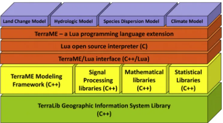
The TerraME architecture is shown inFig. 1. Its lowest tier uses the TerraLib Cþþ library (Câmara et al., 2008). The second tier provides support for modeling in Cþþincluding agent-based, cell-space, systems-oriented and event-based paradigms. The third tier is the interface between TerraME and Lua. It adds data types and functions for model simulation and evaluation to Lua. Other mathematical and statistical libraries can have their APIs exported to the Lua interpreter. The next tier is the Lua interpreter, which takes model source code as input and executes the simulation. The
last tier consists of end user models. The top ofFig. 1shows four examples of models that can be implemented using TerraME.
TerraME considers that a model has spatial, temporal, and
behavioral dimensions. The spatial dimension deals with the geographical area under study and the spatial resolution used for data sampling. The behavioral dimension refers to the rules (for example, agent behavior) and to the indirect techniques (for example, statistical methods) that represent change. The temporal dimension includes the period considered by the model and the frequency when change occurs. To define a model, the user sets up instances of TerraME’s spatial, behavioral, and temporal types, which are described below.
3.2. Spatial types
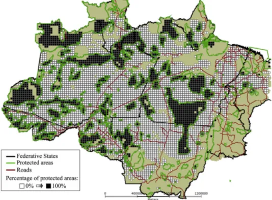
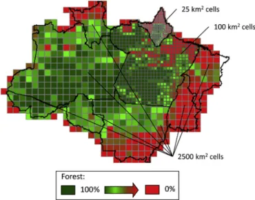
TerraME provides four spatial types:Cell,CellularSpace, Neigh-borhood, and Trajectory. A cell is a spatial location which has persistent and runtime attributes. Persistent attributes are stored in geospatial databases, while runtime values exist only during the simulation. A cellular space is a set of cells representing a geographical area divided in regular or irregular partitions. Cellular spaces can be saved and recovered from TerraLib databases. Each entity of a geospatial database (cell, pixel, point, line, or polygon) is loaded as a cell in TerraME.Fig. 2 shows a database with three different layers: (1) a set of roads represented as lines, (2) Brazilian states within Amazonia represented as polygons, and (3) 2525 km cells composing a sparse grid representing protected areas in Amazonia. Each of them can be read into a cellular space. The third spatial type isNeighborhood, a topological represen-tation of proximity relations. A neighborhood is a set of pairs (c,w), wherec is a neighbor cell and wis the weight of the relation. Neighborhoods connect cells inside the same cellular space or be-tween spaces. Each cell can have more than one neighborhood. TerraME has functions to create simple neighborhoods such as Moore and von Neumann. Complex spatial relations use a gener-alized proximity matrix (GPM). A GPM is a directed graph whose weights express relations between geographic objects (Aguiar, 2006) that can be loaded from a TerraLib database during simula-tions. TerraME does not work with vector geometries explicitly as most operations over such geometries are computationally inten-sive tasks. This is a limitation, but it has the advantage of not computing spatial operations repeatedly during simulations, which reduces computational cost.Fig. 3shows different types of neigh-borhoods. Upper tiles show Moore neighneigh-borhoods. The lower ones depict neighbors built from roads using a GPM.
TerraME supports any algorithm that uses a Euclidean repre-sentation of space. During simulations, it is possible to compute raster-based operations using the (x, y) positions of cells.
Neighborhood relations from exogenous vector-based data, such as connectivity to markets through roads, can change by loading GPMs registered for different simulation times. Once relations are already stored infiles, loading them in different executions of the model reduces simulation time because they do not need to be computed repeatedly.
The fourth spatial type,Trajectory, allows the user to define how to go through a cellular space. A trajectory is an iterator that selects a subset of a cellular space and defines an order for traversing this subspace. Defining trajectories is especially useful for allocating change in space. For example, consider a land change model where the user is interested in modeling the transition from forest to agriculture. The modeller can define a trajectory by selecting all
cells representing forest and ordering them by their potential for change. Cells with higher potential can then be traversedfirst.
3.3. Behavioral types
To describe model behavior, TerraME has two types:Agent and Automaton. Agents are uniquely identifiable individuals situated in space. They can represent actors, institutions, or even whole sys-tems. Each agent has a state, can move over cellular spaces, and can communicate with other agents. TerraME provides functionalities to agents such as synchronous and asynchronous messages, con-nections to cells and other agents, and life span. For model devel-opment, agents can be grouped in aSociety. A society is a collection Fig. 2.Squared cells representing a cellular space for Brazilian Amazonia.
of agents with the same set of properties and temporal resolution. Societies can be created from scratch or retrieved from geospatial databases during the simulation. An agent is related to a society as a cell is to a cellular space.
Anautomatonis a spatial process that has independent states at each location. While an agent acts globally in the cellular space, the automaton acts locally. A single agent with a unique internal state can control several cells. An automaton has many instances that share the same set of states and attributes, but change indepen-dently from each other. At a given time, each instance of an au-tomaton can be in a different state and have different attribute values.
TerraME supports both agents and automata because of the different needs of natureesociety modeling. Societal models need agents that can move freely in space and interact with other agents. By contrast, many natural models (such as hydrological ones) need local variations of global laws. The physical laws are the same, but the local behavior is constrained by natural variations. Thus, the automaton type is better suited for modeling natural processes.
3.4. Temporal types
Once spatial structures and behavioral rules are described, it is necessary to define temporal structures. TerraME has two temporal types:EventandTimer. An event is a time instant when the simu-lation engine executes operations. A timer is a clock that registers a continuous simulation time. It manages an event queue ordered according to their priorities and timestamps. Fig. 4 shows how event scheduling works in TerraME. It contains a timer with a queue of four events. As each event is removed from the head of the queue, the timer’s clock is updated with its timestamp. After that, the event’s action is executed and the event may be deleted or requeued according to its result.
3.5. The environment type
In TerraME, the Environment type allows the user to set up multi-scale models. An Environment represents a micro-world containing data and commands to be executed. It includes the spatial, behavioral, and temporal parts of a model. Environments can be nested, supporting multi-scale models. Thus, combining different environments, users can build complex models.
When developing multi-scale models, the userfirst defines one environment for each model. Then, the internals of each environ-ment are set by defining appropriate instances of TerraME’s types. Breaking up a multi-scale model in different and independent
environments favors interdisciplinary research. Each environment may use a different combination of disciplinary knowledge.Fig. 5 shows one environment that covers the whole Amazon region with 50 50 km2 cells. It has two nested environments, one modeling the Pará state at 1010 km2and the other modeling the Amapá state at 55 km2.
3.6. Calibration and high performance tools
TerraME provides a genetic algorithm for model calibration. It optimizes model parameters to find the best adjustment, using goodness of fit metrics to avoid local minima. It can calibrate several parameters simultaneously, even when the model is sto-chastic and the error function is noisy (Fraga et al., 2010). Currently, we are using the goodness-of-fit measure proposed byCostanza (1989). Future versions of TerraME will include other goodness-of-fit metrics and optimization methods to improve calibration. We have also built a high performance layer to use multiple cores in shared memory architectures. High performance services can be used during model calibration to explore larger search spaces (Silva et al., 2011). A version for distributed memory architectures is currently under development.
4. Examples of dynamic models in TerraME
This section shows case studies that explore the functions of TerraME. We focus mainly on the toolbox instead of showing details of each model.
4.1. A simple land change model
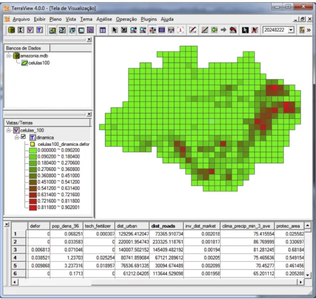
Thefirst example is a land change model whose spatial support is a cellular space of 2525 km2cells representing the Brazilian Amazonia rain forest (shown inFig. 6). This model is a simplified version of the model developed by (Aguiar, 2006).
Thefirst part of the model (shown inFig. 7) describes the spatial entities. An object of typeCellularSpaceis created to read data from the Amazonia database. It requires a database location, the name of the theme within the database, and the attributes to be read. The “amazonia”CellularSpaceconnects to a Microsoft Access database and loads the attributes“percent_defor”(percentage of deforesta-tion, from zero to one), “distance_urban” (distance to urban (1) Get first EVENT
1:32:00 cs:load( ) (2) Update current time
1:32:10 ag1:execute( )
1:38:07 ag2:execute( )
1:42:00 cs:save() (2) Update current time
(3) Execute the ACTION ()
. . .
(4) ACTION return valuefalse
return valuetrue
(5) Schedule EVENT again
Fig. 4.Timer and event, the temporal types of TerraME.
centers),“inv_distance_market”(inverse of the square of distance to markets), and“protection_area”(percentage of protected areas in the cell). These attributes are read for all cells. The last line de-fines a Moore neighborhood for each cell.
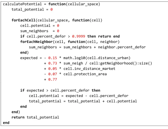
Once the attributes are read into the cellular space, we define a function called calculatePotential()to estimate the deforestation potential of each cell, as shown inFig. 8. It takes a cellular space as argument and uses the second order functionsforEachCell()and
forEachNeighbor(). A second order function takes an object and another function as arguments and applies this function to every element of the given object. We use forEachCell() totraverse a
cellular space, applying a function to all cells. Inside this function, we callforEachNeighbor()to traverse the neighborhood of each cell. In this example,forEachNeighbor()is used to sum the deforestation of all neighbors of a cell. The expected deforestation for each cell is a weighted sum of the average deforestation of its neighbors, its distance to urban centers, its connection to markets, and its per-centage of protected areas. Each cell will get a new attribute called
potentialthat represents its deforestation potential, computed as the difference between the expected deforestation and the current deforestation. The function returns the total potential for change, calculated as the sum of each individual potential.
Fig. 6.Brazilian Amazonia database. The attribute percentage of deforestation is used to color the map, with green representing the cells with forest and red the percentage of deforestation. (For interpretation of the references to color in thisfigure legend, the reader is referred to the web version of this article.)
After calculating the potential of each cell, the model allocates 30,000 km2of deforestation in the Brazilian Amazonia over a 50-year time span. To do this, it uses the algorithm presented inFig. 9, which takes a cellular space and its total potential for change as inputs. It
defines atrajectoryto traverse the cells that have a positive defores-tation potential, running from higher to lower potential values. To select the cells with positive potential for change, it uses the parameterfilter. By taking the attribute“potential”as reference, the Fig. 8.Land change potential procedure.
parametersortarranges the cells from higher to lower potential values. The deforestation area of each cell is then allocated as a function of its potential for change. There is an extra check to avoid the percent of deforestation of a cell going over 100%. Deforestation takes place until at least 99.9% of the initial demand has been allocated.
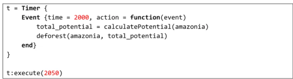
To wrap up the model, we define its temporal component, composed by atimerwith a singleevent, as shown inFig. 10. The event callscalculatePotential()to compute the potential and then
deforest()to allocate deforestation. The simulation starts in 2000 and runs until 2050.Fig. 11shows three parameters of the model and the evolution of deforestation along a simulation.
4.2. A multi-scale continenteoceaneatmosphere model
The second example simulates a water cycle involving atmo-sphere, continent, and ocean, as follows:
Water in the continentflows by gravity into the ocean;
The height of the ocean is kept the same among its cells;
Water in the ocean evaporates to the atmosphere;
Water vapor in the atmosphere goes to higher altitudes by convection;
High concentrations of water vapor turn into rain, moving water from the atmosphere to the continent.
The model has three cellular spaces. The atmosphere has a spatial overlay with continent and ocean, while some cells in the border of the continent touch other cells in the ocean.Fig. 12shows the layers and the waterflows.
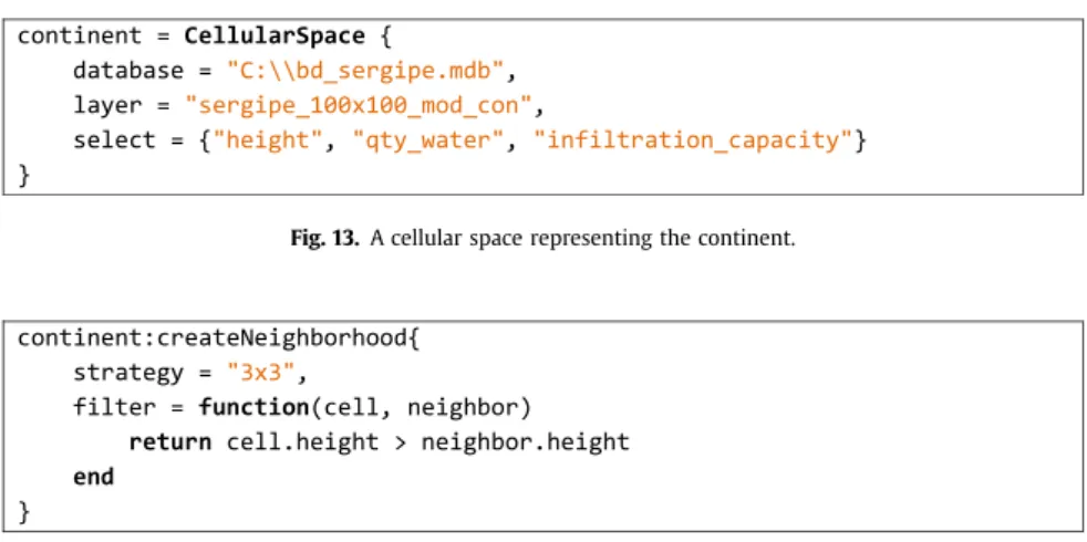
Thefirst step to implement this model is to define three cellular spaces (ocean,athmosphere, andcontinent).Fig. 13shows the source code for reading the continent cellular space from a database. The continent has three attributes: height, quantity of water, and infiltration capacity. The other cellular spaces are created in a similar way.
The next step defines the neighborhoods. In the continent, the neighborhood of a cell depends on its height and that of its adjacent cells. Only cells with a lower height belong to a cell’s neighborhood. This strategy sets up a local drainage direction for each cell to simulate the waterflow by gravity.Fig. 14shows the code to create the continent’s neighborhood using afilter over a 33 neighbor-hood. In the end of this procedure, cells where all 33 neighbors are higher will have no neighbors. Such cells correspond to depression areas.
We also need to set connections between cellular spaces to simulate evaporation, precipitation, and discharge. Fig. 15shows how to connect the atmosphere to the continent using crea-teNeighborhood(). The argumenttargetindicates that a connection will be created between cellular spaces, from the one that calls the function to its target. The geometric matching between the cellular spaces is defined by the argumentstrategy. The strategy“coord” connects two cellular spaces whose spatial positions are the same. Other connections in the model are created similarly. As we have more than one neighborhood associated to each cell, we need to give a name to the new neighborhood. In this case, the name is “atmosphere_continent”.
After describing the spatial entities and connecting them, we now set the waterflows. For the sake of simplicity, we show only Fig. 10.A timer with a single event to simulate deforestation.
the continent’s behavior, as the other cellular spaces use similar strategies. Waterflows downstream (runoff) and also permeates the continent (infiltration). We express these two processes sepa-rately in the model.
In the runoff calculation, water in the higher cellsflows to the lower ones. Recall the continent’s neighborhood is a local drainage. Using the neighborhood, we divide the waterflow from a cell to its neighbors, as shown inFig. 16. To compute the waterflows, we need to keep two copies of each cell. One contains the water that will flow out of the cell. The other will receive water from upstream neighbors, which will be kept for the next iteration. For this pur-pose, TerraME has two versions of the attributes of a cellular space in memory. One stores past values of each cell’s attributes, while the other stores the current (updated) values. This helps to simulate processes that occur in parallel in space. Past attributes are read only, as changes take place in the current time. Before updating the cells, it is necessary tosynchronize()the cellular space. This updates the past values with the current attributes, so we can start another simulation step.
Water infiltration to the continent is a continuous process that needs to be discretized within the simulation. It is described as an event-driven function that computes a numerical integration al-gorithm using the built-in functionintegrate(), as shown inFig. 17. When the simulation triggers the event to execute water infi ltra-tion, the integration is computed for each cell using the period between the current time and the last time the event was executed. The main parameter ofintegrate()is theequationto be integrated. In this example, the numerical integration uses an infiltration()
function that states the water in a cell will be reduced by 0.03 units
per unit of time. The other arguments are the integrationmethod
(“euler”), aninitialvalue, the triggeringevent, and the integration
step.
After creating the behavior within the continent, we define temporal entities.Fig. 18shows the timer that controls the conti-nent’s simulation. It has two events, which may haveprioritiesto define their execution order. Lower values denote higher priority, with zero being the default value. Thefirst event simulates water balance flows in the continent, while the second simulates the water infiltration. This timer and the cellular space representing the continent are then joined to make up an Environment. Using similar procedures as those that set up the continent environment, we can create the ocean environment and the atmosphere environment.
The next step describes how water moves between cellular spaces: discharge (continent to ocean), rain (atmosphere to conti-nent), and evaporation (ocean to atmosphere).Fig. 19describes the source code for the water discharge. As water arrives in the lower cells on the border of the continent, the model sends water from the continent to the ocean. In this case, functionsgetNeighborhood()
and forEachNeighbor() use the name of the neighborhood that connects the continent to the ocean as their argument.
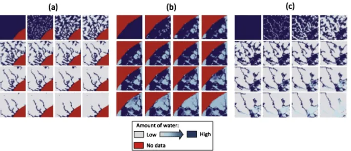
The three environments (ocean, continent, and atmosphere) are enclosed in a global one, as shown inFig. 20. The global environ-ment also has a timer that triggers events to distribute the initial flow of water, make it rain, and execute evaporation and discharge. The event that executes rain has a parameterperiodto indicate that it will execute three times less frequently than the other events. To change the amount of rain along the simulation, one could change functionexecute_rain() or reduce its periodicity. Finally, we set the global environment to be executed until time 2000. During the simulation, the global environment synchronizes the timers so that all events occur in the correct order.Fig. 21shows theflow of water in each cellular space at the end of a simulation. It is possible to see the emergence of global patterns of water from the local rules defined by the model.
4.3. A simple predatoreprey model
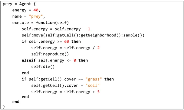
The last example describes a predatoreprey model using an agent-based approach. In this model, preys and predators are represented as individuals that live in a cellular space. The type
Agentencapsulates the attributes and behavior of autonomous in-dividuals. A prey has two properties, energy and name, and a function,execute(). Energy represents its currentfitness, starting with 50 quanta, while name distinguishes preys from predators. Fig. 12.Atmosphereecontinenteocean database and waterflows.
Fig. 13.A cellular space representing the continent.
Fig. 16.Continent water runoff balance.
Fig. 17.Continent water infiltration.
The functionexecute()has a single parameter representing the prey itself. It describes the actions executed by the prey at each time step. In the beginning, the prey loses one quantum of energy to move from its current cell to a random neighbor. Then it checks its energy. When it has 60 or more quanta of energy, the prey re-produces asexually, creating a descendant in the same cell. When its energy is equal or less than zero, the prey dies. Finally, if there is grass in the cell, the prey feeds on it, converting the cell’s cover from grass to soil to increasing its own energy byfive quanta.Fig. 22 represents the prey agent.
A predator is described similarly. It loses energy, moves, re-produces, and dies in the same way as a prey. The difference is that it looks for preys in the cell it belongs. We useforEachAgent()to go through a collection of agents, applying a function to each one. In this example, we useforEachAgent()to represent how predators feed on preys. A predator looks for a prey in the same cell it is located. If there is a prey, the predator kills and eats it, increasing its energy by half of the prey’s energy. At each time step, the predator stops searching for other preys afterfinding thefirst one (Fig. 23).
Fig. 19.Source code for water discharge.
Fig. 20.The world environment.
The second part of this model creates one society ofpredators,
one of preysand a cellular space where they will be located. The agents defined previously are used as prototypes that will be cloned to create bothsocieties. In the example, both societies have 200 agents cloned from their respective prototypes. The model also creates an environment composed by the cellular space and the societies. To put agents in the cellular space, we call the function
createPlacement()using a random strategy. A timer defines cycles of preys, predators, and grass regrowth (Fig. 24).
The initial distribution of agents and the result of one simu-lation are shown inFig. 25. Green cells arefilled with grass. Black asterisks represent preys, while red asterisks represent preda-tors. In the beginning, all of the cells are green since the cellular space isfilled with grass. As the simulation proceeds, preys feed grass, which changes the color of cells to white. The number of agents within each society also changes, as they feed, reproduce, and die.
5. Discussion andfinal remarks
In this section, we consider the lessons learned when designing TerraME. We start by recalling our conjectures: a toolkit for modeling natureesociety interactions needs to provide a set of data types with methods to build and connect geospatial micro-worlds. Thus, the lowermost level of TerraME has two data types:Celland
Agent. Cells represent the spatial partitions, with attributes that capture the variations of the natural and the human-built worlds. Agent represents autonomous individuals that can change the landscape. Two containers come right above both types. A set of cells representing a geographic area of interest with a given reso-lution and extent makes up aCellularSpace. A set of agents that have the same set of attributes and basic behavior compose aSociety. Both sets can have their entities loaded directly from a geospatial database, which simplifies dealing with real-world data. Some simulation toolkits have added interfaces to geospatial databases as Fig. 22.Describing a prey as an agent.
an extension from their original concepts. By contrast, manipu-lating geospatial data is native in TerraME.
Another innovation in TerraME is the idea of environment. An environment represents a micro-world with one or more cellular spaces and one or more societies. Inside an environment, there is temporal coherence between its events. Using the idea of envi-ronments, models can be composed of sub-models with different spatial and temporal resolution and behavior. This bottom-up logic allows for considerableflexibility. Simple models can be built using a single cellular space or a single society, without the need to define environments. Complex models will use environments to imple-ment micro-worlds separately and couple them.
TerraME’sflexibility comes at a price, however. To understand why, consider some of the alternative toolkits. If the user’s problem can be expressed as sets of operations over maps, then map algebra toolkits such as PCRaster (Karssenberg et al., 2001) provide higher-level operations. Instead of iterating over every cell of a map as TerraME does, map algebra functions take a map (or a cellular space) as an atomic unit. Single statements in map algebra need a considerable number of lines in TerraME. Nevertheless, if the
problem requires combining agents with maps, it is probably easier to express such models in TerraME than in a map algebra toolkit.
We recognize that prospective users will pay a price for the flexibility provided by TerraME. The learning curve will be steeper than that of a single-paradigm model. Also, there are no previous examples of similar tools that the user is likely to be familiar with. All of this may place a barrier for first-time users of TerraME. Nevertheless, we consider that there is space for a multi-paradigm modeling tool. Some problems will be too complex tofit in a single paradigm. Also, users that want to combine different approaches can benefit for having these concepts supported in a single tool.
When comparing natureesociety modeling tools, it is useful to consider the lessons learned from programming languages in general. It is unlikely that a single programming language willfit the needs of all software developers. There is room for scripting, object-oriented, functional and multi-paradigm languages. The same view applies to modeling. The community will benefit for multiple solutions. We believe that TerraME is a new approach to natureesociety modeling, which will find its niche alongside existing and mature tools.
Fig. 24.Societies and other objects for the predatoreprey model.
improving the paper.
References
Aguiar, A.P.D., 2006. Modeling Land Use Change in the Brazilian Amazon: Exploring Intra-regional Heterogeneity. PhD thesis. In: Remote Sensing Program. INPE, Sao Jose dos Campos.
Batty, M., 2012. A generic framework for computational spatial modelling. In: Heppenstall, A., Crooks, A., See, L., Batty, M. (Eds.), Agent-based Models of Geographical Systems. Springer, Dordrecht, NL, pp. 19e50.
Beven, K., Binley, A., 1992. The future of distributed models: model calibration and uncertainty prediction. Hydrological Processes 6 (3), 279e298.
Câmara, G., Vinhas, L., Ferreira, K., Queiroz, G., Souza, R.C.M., Monteiro, A.M., Carvalho, M.T., Casanova, M.A., Freitas, U.M., 2008. TerraLib: an open-source GIS library for large-scale environmental and socio-economic applications. In: Hall, B., Leahy, M. (Eds.), Open Source Approaches to Spatial Data Handling. Springer, Berlin, pp. 247e270.
Costanza, R., 1989. Model goodness of fit e a multiple resolution procedure.
Ecological Modelling 47 (3e4), 199e215.
Crooks, A., Castle, C., 2012. The integration of agent-based modelling and geographical information for geospatial simulation. In: Heppenstall, A., Crooks, A., See, L., Batty, M. (Eds.), Agent-based Models of Geographical Sys-tems. Springer-Verlag, Heidelberg.
Eberlein, R.L., Peterson, D.W., 1992. Understanding models with Vensim (TM). Eu-ropean Journal of Operational Research 59 (1), 216e219.
Filippi, J., Bisgambiglia, P., 2004. JDEVS: an implementation of a DEVS based formal framework for environmental modelling. Environmental Modelling and Soft-ware 19 (3), 261e274.
Forrester, J.W., 1961. Industrial Dynamics. MIT Press, Cambridge, MA.
Fraga, L., Carneiro, T., Lana, R., Guimarães, F., 2010. Calibração em Modelagem Ambiental na Plataforma TerraME usando Algoritmos Genéticos (Enviromental Modelling Calibration using TerraME using Genetic Algorithms), 42 Brazilian Symposium on Operations Research, Bento Gonçalves, Brazil.
Gray, J., 1981. The transaction concept: virtues and limitations. In: 7th International Conference on Very Large Data Bases (VLDB). IEEE Computer Society, Cannes, France, pp. 144e154.
Ierusalimschy, R., Figueiredo, L.H., Celes, W., 1996. Luaean extensible extension
language. Software: Practice & Experience 26 (6), 635e652.
Jakeman, A.J., Letcher, R., Norton, J., 2006. Ten iterative steps in development and evaluation of environmental models. Environmental Modelling & Software 21 (5), 602e614.
Janssen, P.H.M., Heuberger, P.S.C., 1995. Calibration of process-oriented models. Ecological Modelling 83 (1e2), 55e66.
Karssenberg, D., Burrough, P.A., Sluiter, R., de Jong, K., 2001. The PCRaster software and course materials for teaching numerical modelling in the environmental sciences. Transactions in GIS 5, 99e110.
Moran, E.F., 2010. Environmental Social Science: HumaneEnvironment Interactions
and Sustainability. Wiley-Blackwell, Malden, Mass.
Muetzelfeldt, R.I., Massheder, J., 2003. The Simile visual modelling environment. European Journal of Agronomy 18, 345e358.
North, M.J., Collier, N.T., Vos, J.R., 2006. Experiences creating three implementations of the repast agent modeling toolkit. ACM Transactions on Modeling and Computer Simulation 16 (1), 1e25.
Parker, D.C., Manson, S.M., Janssen, M.A., Hoffmann, M.J., Deadman, P., 2003. Multi-agent systems for the simulation of land-use and land-cover change: a review. Annals of the Association of American Geographers 93 (2), 314e337.
Pontius Jr., R.G., Millones, M., 2011. Death to Kappa: birth of quantity disagreement and allocation disagreement for accuracy assessment. International Journal of Remote Sensing 32 (15), 4407e4429.
Rindfuss, R.R., Walsh, S.J., Turner, B.L., Fox, J., Mishra, V., 2004. Developing a science of land change: challenges and methodological issues. Proceedings of the Na-tional Academy of Sciences 101 (39), 13976e13981.
Roberts, N., Anderson, D., Deal, R., Garet, M., Shaffer, W., 1983. Introduction to Computer Simulation: a System Dynamics Modeling Approach. Addison-Wes-ley., Reading, MA.
Silva, S., Lima, J., Carneiro, T., 2011. Parallel Calibration of Spatial Dynamic Models in TerraME, IADIS. International Conference on Applied Computing Rio de Janeiro, Brazil, pp. 451e456.
Steiniger, S., Bocher, E., 2009. An overview on current free and open source desktop GIS developments. International Journal of Geographic Information Science 23 (10), 1345e1370.
Stroustrup, B., 1994. Design and Evolution of Cþþ. Addison-Wesley, New York. Tisue, S., Wilensky, U., 2004. NetLogo: a Simple Environment for Modeling
Complexity. Boston: International Conference on Complex System.
Tomlin, C.D., 1990. Geographic Information Systems and Cartographic Modeling. Prentice-Hall, Englewood Cliffs, NJ.
Turner, B., Skole, D., Sanderson, S., Fischer, G., Fresco, L., Leemans, R., 1995. Land-use and Land-cover Change (LUCC): Science/Research Plan, HDP Report No. 7. IGBP Secretariat, Stockholm.
Verstegen, J.A., Karssenberg, D., Van der Hilst, F., Faaij, A., 2012. Spatio-temporal uncertainty in Spatial Decision Support Systems: a case study of changing land availability for bioenergy crops in Mozambique. Computers, Environment and Urban Systems 36 (1), 30e42.
von Neumann, J., 1966. In: Burks, A.W. (Ed.), Theory of Self-reproducing Automata. Illinois.
Wesseling, C.G., Karssenberg, D., Van Deursen, W.P.A., Burrough, P.A., 1996. Inte-grating dynamic environmental models in GIS: the development of a Dynamic Modelling language. Transactions in GIS 1, 40e48.
White, R., Engelen, G.,1997. Cellular automata as the basis of integrated dynamic regional modelling. Environment and Planning B: Planning and Design 24, 235e246.
Wooldridge, M.J., Jennings, N.R., 1995. Intelligent agents: theory and practice. Knowledge Engineering Review 10 (2).