REPOSITORIO INSTITUCIONAL DA UFOP: Is the pseudogap a topological state?

Current Perspectives

Is the pseudogap a topological state?

Alfredo A. Vargas-Paredes

a,n

, Marco Cariglia

b

, Mauro M. Doria

c

a_{Departamento de Física, Universidade Federal Rural de Pernambuco, 52171-900 Pernambuco, Brazil} b_{Departamento de Física, Universidade Federal deOuro Preto, 35400-000 Ouro Preto Minas Gerais, Brazil} c_{Departamento de Física dos Sólidos, Universidade Federal do Rio de Janeiro, 21941-972 Rio de Janeiro, Brazil}

a r t i c l e

i n f o

Article history:

Received 19 May 2014 Received in revised form 15 September 2014

Available online 22 September 2014

Keywords: Magnetism Superconductivity Pseudogap Order parameter Skyrmion

a b s t r a c t

We conjecture that the pseudogap is an inhomogeneous condensate above the homogeneous state whose existence is granted by topological stability. We consider the simplest possible order parameter theory that provides this interpretation of the pseudogap and study its angular momentum states. Also we obtain a solution of the Bogomol'nyi self-duality equations andfind skyrmions. The normal state gap density, the breaking of the time reversal symmetry and the checkerboard pattern are naturally explained under this view. The pseudogap is a lattice of skyrmions and the inner weak local magnetic

field falls below the experimental threshold of observation given by NMR/NQR and

μ

SR experiments.

&2014 Elsevier B.V. All rights reserved.

1. Introduction

The discovery of the high temperature (highTc) superconduc-tors by Bednorz and Müller (1986)[1]brought new paradigms to the_field of condensed matter physics. Three-dimensional super-conductivity originates in two-dimensional layers where Cooper pairs are formed and outlive elsewhere. The understanding of any layered compound demands its study at several doping, achieved by changing the number of carriers available in the layers. These properties are best displayed in the so-called temperature versus doping diagram where the critical temperatureTcdefines a dome shaped curve whose onset and disappearance take place at critical doping values. In this phase diagram superconductivity is one among many other possible electronic states that involve mag-netic, charge and pairing degrees of freedom that either coexist, cooperate or dispute the same spatial locations within the layers. Besides the superconducting and the anti-ferromagnetic state there is another characterized electronic state, the pseudogap state, that lives below a temperatureTn

versus doping line in this phase diagram. Interestingly this line approaches the supercon-ducting dome from above by increasing the doping, always with a negative slope and, at some doping value, intersects and crosses the dome, ending at zero temperature, where it defines a so-called quantum critical point. The pseudogap was revealed in 1989, soon

after the discovery of Bednorz and Müller, by the observation of a sharp decrease of the nuclear spin susceptibility in the cuprate layer atoms (CuO2)[2]. This sharp decrease of the NMR Knight shift K indicated the existence of a (aboveTc) normal state gap, the pseudogap. The nature of the pseudogap remains so far unknown and a true challenge to the field. It is not clear whether the pseudogap gap lineTn

is a thermodynamical or crossover transi-tion[3]. Among the known properties of the pseudogap, are the normal state gap and the spontaneously broken symmetries. The pseudogap state breaks the time reversal symmetry because left-circularly polarized photons give a different photocurrent from right-circularly polarized photons below the line Tn

, as shown more than 10 years ago by Kaminski et al. [4]. Recently these results have been con_firmed through high precision measure-ments of polar Kerr effect[5,6], which are also clearly suggestive of a phase transition atTn

, below which arises afinite Kerr rotation [7]. The pseudogap also breaks translational invariance symmetry within the layers and this modulation wasfirst observed through scanning tunneling microscopy, initially coined as the checker-board pattern, a tetragonal lattice with 4aperiodicity, whereais the CuO2unit cell length. This periodicity wasfirstly found inside the vortex cores[8]of Bi2Sr2CaCu2O8þx, butsoon after incommen-surate patterns were also observed in the normal state of this compound [9], below the pseudogap line in the absence of a magneticfield. It is quite remarkable that in the pseudogap phase carriers within the layers arrange themselves into a periodic pattern not necessarily commensurate with the crystallographic Contents lists available atScienceDirect

journal homepage:www.elsevier.com/locate/jmmm

Journal of Magnetism and Magnetic Materials

http://dx.doi.org/10.1016/j.jmmm.2014.09.042 0304-8853/&2014 Elsevier B.V. All rights reserved.

n

Corresponding author.

E-mail address:[email protected](A.A. Vargas-Paredes).

structure[10]. Nowadays the checkerboard pattern is seen as a consequence a charge density wave [11]. Recent work using resonant elastic x-ray scattering (REXS) correlation done by Ghiringhelli et al. [12] found concrete evidence of this charge-density-wave in the underdoped compound YBa2Cu3O6þxwith an incommensurate periodicity of nearly 3.2a, both above and below Tc. Thus it is quite clear that a theoretical attempt to explain the pseudogap must take into account the normal state gap and also the broken symmetries. It happens that a magnetic order is expected to arise due to the breaking of the time reversal symmetry. Time reversal symmetry means that a state remains unchanged upon time reversal. We know that the velocity (mo-mentum) and also the magnetic_field both reverse sign under a time-reversal operation. Magnetic spins reverse direction when time reverses direction, therefore magnetic order breaks time reversal symmetry and may be the reason for it. The presence of any kind of magnetic order leads to a local magnetic field that must be experimentally accessed by several magnetic probes. Indeed there has been an intense search for this predicted spontaneous local magneticfield inside the highTc superconduc-tors in the pseudogap phase. Polarized neutron diffraction experi-ments [13,14] indicate a magnetic order below the pseudogap. NMR/NQR[15,16]andμSR[17,18]experiments set an upper limit to the magneticfield between the layers, which must be smaller than 0.1 Gauss. A proposal of magnetic order with the layers has been put forward by C.M. Varma[13,14,19,20], who claims that microscopic orbital currents cause this order, and consequently, the breaking of the time reversal symmetry.

Recently we have shown that an above the homogeneous (normal) state gap and the broken symmetries can be understood in the context of an order parameter description, and for this reason, suggested this interpretation for the pseudogap[21]. Thus the pseudogap is a gapped topological state made of skyrmions, whose microscopic nature is still controversial. We recall that the description of a condensate through an order parameter was proposed by Ginzburg and Landau much before the BCS unveiled the microscopic mechanism behind superconductivity. According to Gorkov and Volovik [22] a system described by an order parameter that breaks the time reversal symmetry must have an accompanying magnetic order that yields a local magneticfield near to the sample surface even in the absence of an externalfield. Indeed our description of the pseudogap exactly_fits the Gorkov and Volovik scenario with the local magneticfield found around the layers and not just near to the sample surface. This magnetic field originates from spontaneous circulating supercurrents in the layers that give rise to an inhomogeneous excited state which is stable since it is prevented from decaying into the homogeneous ground state by its topological stability. This tetragonal lattice of skyrmions breaks time reversal symmetry and also translational invariance has an energy gap above the homogeneous state that we associate to the pseudogap. We obtain the numerical value of the pseudogap density as a function of the local magneticfield between the layers, which is assumed to fall below the experi-mental threshold of observation set by NMR/NQR[15,16]andμSR

[17,18]experiments. In this paper we provide a detailed study of this order parameter approach to the pseudogap state and derive its angular momentum properties.

2. The theory

We seek here the simplest possible theory able to describe a condensate, the pseudogap, through an order parameter such that it lies above the homogeneous state separated by a gap, hereafter called the normal state gap, and presents broken symmetries. Besides the supercurrents created by its inhomogeneity must be in

conformity with the experimental threshold imposed by the maximum observed internalfield. Because of its assumed simpli-city the present theory does not describe the transition at Tn

, as we only try to capture the major qualitative features of the pseudogap. Thus the present description is restricted to tempera-tures below but near to theTn

line, and aboveTc, such that the condensate energy, which regulates the superconducting dome and defines Tc, can be safely ignored. Thermal fluctuations are not included here and so the discussion is restricted to mean field considerations. Even in this simpli_fied context we_find that to describe both the pseudogap and the superconducting states there must be at least two components,Ψ=

( )

ψψ

u

d . This simplest

possible theory is just the sum of the kinetic and thefield density energies

⎡

⎣ ⎢ ⎢ ⎢

⎤

⎦ ⎥ ⎥ ⎥

∫

Ψ

π

= |

→ |

+ →

F d x

V D

m h

2 8 ,

(1)

3 2 2

wheremandqare the Copper pair mass and charge, respectively. We assume minimal coupling to thefield through the covariant derivative→D =( / )= i →∇−( / )q c A→ and→h = ∇→×→A. Undoubtedly the lowest free energy state of Eq.(1)is the null homogeneous state Ψ=0, thus with no supercurrents and no resulting local magnetic field, →h =0 that we identify with the superconducting state restricted to exist under the superconducting dome. Our claim is that above this homogeneous null state lives an inhomogeneous gapped state, topologically stable, conjectured to be the pseudo-gap. In this paper we give a detailed derivation of the pseudogap from Eq.(1)and obtain its angular momentum properties.

This simple theory has a global SU(2) rotational invariance [23,24]that arises as a natural consequence of the presence of two-components. We believe that this invariance is explicitly broken by extra terms in the free energy, not considered in this simple theory. Even without considering this explicit breaking we find that this naively introducedSU(2)symmetry has possibly only local meaning and is associated to the group of spatial rotations, which turns Ψ into a truly spinorial order parameter. It is not possible to bring the two-component order parameter into a one-component form, Ψ′ =UΨ, Ψ′ =T (ψ′ 0) _{by an SU(2) rotation,}

=

†

UU 1in case of an inhomogeneous state. It is only possible to get rid of one of the components in case of an homogeneous solution. For a spatially inhomogeneous solution,Ψ( )→x , the rota-tion to one component form can only be done locally, U x( )→. Therefore the free energy of Eq. (1) cannot be reduced to one component in case of an inhomogeneous solution. Under a local rotationU x( )→ an extra term appears in the covariant derivative,

→

′ =→+ → −

D D UD U 1_{so thatF =}

_∫

_{d x D(| ′}→_{Ψ′|/2 )/m V} k

3 2

. We consider this a signal of a non-abelian gauge symmetry in the pseudogap phase. This possibility has been considered elsewhere[25,26]but will not be treated here. From the free energy of Eq. (1) we obtain the following variational equations:

Ψ →

= D

m

2 0, (2)

2

π ∇

→

×→h = → c J 4

,

(3)

where the supercurrent density is given by

⎡ ⎣⎢

⎤ ⎦⎥ Ψ Ψ Ψ Ψ →

= †→ + → †

J q

m D (D ) . (4)

the above equations. The local magneticfield itself works as the small parameter helpful to solve these equations recursively by the following procedure. The order parameterΨ is obtained from Eq. (2)neglecting the interaction with thefield, which means that the equation to solve is truly→∇2Ψ=0. Once in power of this solution Ψ, and the supercurrent obtained in this order, Eq.(3)is used to derive→h from a known source. This iterative procedure is repeated recursively, and so, de_fines a perturbative scheme. We carry it just to the first iteration, which means that the local magnetic field must be very weak. Another important ingredient to added in our search of the solution of the above equations is the geometry, namely a stack of layers, such that the order parameter is assumed to evanesce away from each one of them. Thus we seek a Fourier solution of→∇2Ψ=0,Ψ=_ei k x→·→+k x Ψ_→

k k

( )

( , ) 3 3

3, where the wave vector

along the layer is →

≡ ˆ + ˆ ≡ |→|

k k x1 1 k x2 2, and k k. (5)

This solution must satisfy|→k| +2 k3=0

2

between layers, therefore displaying evanescence away from the layers means thatk3= ±ik.

To be of finite energy, the order parameter is chosen Ψ=_ei k x→·→− | |k x Ψ_→

k

( ₃) _{for a layer at}

=

x3 0. Thus between the layers

the order parameter does not vanish, which means that the present treatment assumes a metallic medium and not a vacuum. InterestinglyΨ solves→∇2Ψ=0 above and below but not at the layer itself (x3=0). The Fourier coefficientsΨ→k are so far free, and

can be determined through the angular momentum properties of the order parameter.

Although the above scheme contains the basic sought ideas, it does not unfold the topological stable solutions that exist in the layered system. To unveil them a dual view of the kinetic energy [21]must be obtained, as shown in the next section.

3. The dual view of the theory

In this section we construct a dual formulation of the kinetic energy density. To make our demonstration clearer we express three-dimensional indices explicitly such that repeated indices mean a summation according to the Einstein convention

Ψ

Ψ δ Ψ |→D | ₌ †

m m D I D

2 1

2 ( i ) ij ( j ), (6)

2

and introduce the two-dimensional identity

⎛ ⎝

⎜ ⎞

⎠ ⎟ =

I 1 0

0 1

and the Clifford algebra associated to the Pauli matrices s_i, =

i 1, 2, 3

σ σ = δ

{

i, j

}

2 ijI, ₍₇₎

σ σ = iε σ

[ ,i j] 2 ijk k. (8)

The two-dimensional unity can be expressed in terms of the Pauli matrices

δ =σ σ − ε σ

Iij i j i ijk k. (9)

Then we the kinetic energy acquires a new form

⎡

⎣ ⎢ ⎢

⎤

⎦ ⎥ ⎥ Ψ

σ Ψ ε Ψ σ Ψ |→ |

= | | − †

(

D

m m D i D D

2 1

2 i i ijk( i ) k j ) . ₍₁₀₎

2

2

Manipulation of the second term of the r.h.s of Eq.(10)gives that

= ⎡

⎣⎢

⎤ ⎦⎥ ⎡

⎣⎢

⎤ ⎦⎥ ε Ψ σ Ψ

Ψ σ Ψ Ψ σ Ψ

Ψ σ Ψ Ψ σ Ψ

= − →∇· → × → − → × →

+ →· → × → − → × → ·→

†

† †

† †

D D

i D D

D D D D

( ) ( )

2 ( ) ( )

1

2 ( ) ( ) . (11)

ijk i k j

The antisymmetry of the Levi–Civita symbol allows us to express

=

Ψ σ†→· → × → = − → × → ·→ = −_{D D}Ψ _{D D}Ψ†σ Ψ q→· →Ψ σ Ψ†

ich

( ) ( ) ,

(12)

in terms of→h. Finally we reach the dual view of the kinetic energy

=

= ⎡

⎣ ⎢ ⎢

⎤

⎦ ⎥ ⎥ Ψ σ Ψ

Ψ σ Ψ

Ψ σ Ψ Ψ σ Ψ |→ | ₌|→·→ | ₊ →

· →

+ →∇· → × → − → × →

†

† †

D m

D m

q mch

m D D

2 2 2 ( )

4 ( ) ( ) . ₍₁₃₎

2 2

The last term is a total derivative and yet it is a non-vanishing contribution because of the exponential evanescence of the order parameter away from the layer. In fact we find that this total derivative term describes the normal state gap associated to the pseudogap.

3.1. The variational and thefirst-order equations

The mathematical identity obtained in the previous section is used here to obtain a new perspective of the problem. Using Eq. (13)we can write the free energy of Eq.(1), as follows:

=

= ⎧ ⎨ ⎪

⎩ ⎪

⎡

⎣ ⎢ ⎢ ⎢

⎤

⎦ ⎥ ⎥ ⎥

⎫ ⎬ ⎪

⎭ ⎪

∫

σ Ψ

Ψ σ Ψ

Ψ σ Ψ Ψ σ Ψ π

= |→·

→ |

+ →· →

+ →∇· → × → − → × → + →

†

† †

F d x

V D

m

q mch

m D D

h

2 2 ( )

4 ( ) ( ) 8 .

(14)

3 2

2

Taking the variation of Eq. (14) for δΨ† and δ→A, we obtain the Ginzburg–Landau equation and Ampere's Law with a new vest

σ Ψ μ σ Ψ →·→ = − →·→

( )

m D h

1

2 B (15)

2

⎡ ⎣⎢

⎤ ⎦⎥ πμ Ψ σ Ψ

π

Ψ σ σ Ψ ∇

→

× →+ →

= → →·→ +

†

†

h

q

mc D c c

( 4 )

2

( ) . . .

(16) B

where μ_B==q mc/2 . The surface term of Eq. (14) does not con-tribute to the above variational because it is a total derivative and δ→A =δΨ†=0in the boundaries of integration. This second view of the Ampere's law provides the following formulation of the supercurrent:

= ⎡

⎣⎢

⎤ ⎦⎥

Ψ σ σ Ψ Ψ σ Ψ →

= †→ →·→ + − →∇× †→

J q

m D c c

q m

2 ( ) . 2 ( ). (17)

Next we introduce the weak local magnetic_field approximation, discussed in the previous section, but now applied to the dual view of the theory. However before doing so, we notice a remarkable feature that can only be seen from the above dual variational equations. Ampere's law, as given by Eq.(16), is exactly solved by assuming the followingfirst-order equations:

σ Ψ

→·→ =D 0, (18)

πμ Ψ σ Ψ →

= − †→

h 4 B . (19)

These equations are at the heart of our approach. The solution of Eqs.(18) and (19) is also a solution of the variational equations of Eqs.(15) and (16) provided that the weak local magneticfield approximation is taken into account. In fact Eqs. (18) and (19) provide a precise meaning for the weak local magnetic _field approximation. A scale transformationΨ→εΨ, where

ε

is a small parameter, leaves Eq.(18)invariant. It is Eq.(19)which sets the scale since under this transformation→h →ε2→h. Therefore introdu-cing a solution of thefirst-order equations into Eq.(15)renders its left hand side null and its right hand side of order

ε

3

. In conclusion the variational equations are automatically solved by the _fi rst-order equations in rst-order

ε

3_{. Therefore we solve the}

first-order equations in the lowest possible order instead of the variational equations. We neglect

ε

3 _{corrections to Eq.(18)which means to} solve→·∇σ →Ψ=0instead. Then Eq. (19) determines the magnetic field in order

ε

2_{. Following this program the free energy must be} obtained under the small magneticfield approximation in order

ε

3_{, to be consistent with the order}

_ε

2 _{kept in the variational} equations. Firstly we show that Eq.(18)can be written differently if we multiply it by →σ: → →·→ = − → × → + →σ

(

σ DΨ

)

iσ DΨ DΨ. The first term in the r.h.s is known as the Rashba interaction. Thus the_fi rst-order equation(18)becomes

Ψ σ Ψ →

= → ×→

iD D . (20)

Under this relation Eq.(13)can be expressed as

= Ψ

πμ Ψ σ Ψ Ψ |→ |

= − †→ + →∇ | | D

m m

2 4 B( ) 4 . (21)

2

2 2 2 2 2

If we discard terms of order

ε

4_{or superior only the last term has to} be kept in the kinetic energy. The_field energy is also neglected since it is of order

ε

4_{since it is proportional to the square of the magnetic} field. Consequently the free energy of Eq.(1)becomes in order

ε

3

=

_∫

_Ψ

= →∇ | | F

m d x

V

4 , (22)

2 3 2

2

In the next section we obtain solutions of thefirst-order equations, Eqs. (18) and (19), for a single and multiple layers, respectively. The energy density given by Eq.(22)is shown to describe a normal state gap.

4. The order parameter

4.1. Single layer

The first-order equation for Ψ, Eq. (18), neglecting terms of order

ε

3_{or higher corresponds to}

σ Ψ →·∇→

=0 (23)

sinceΨ∝ε, and→A ∝ε2_{. In components it becomes,} ⎛ ⎝ ⎜⎜ ⎞ ⎠ ⎟⎟⎛ ⎝ ⎜⎜ ⎞ ⎠ ⎟⎟ ψ ψ ∇ ∇ − ∇ ∇ + ∇ −∇ = i

i 0. ₍₂₄₎

u

d

3 1 2

1 2 3

We seek the solution describing a single layer at x3=0 that

vanishes exponentially away from it forx3<0andx3>0 ⎛ ⎝ ⎜ ⎜ ⎞ ⎠ ⎟ ⎟

∑

Ψ ψ ψ = → ≠ − | | → →

e e k

k ( ) ( ) ,

(25) k

k x i k x u

d 0

. 3

The→k =0 component is excluded since it describes a constant homogeneous order parameter, assumed not to exist here. To

obtain a relation between

ψ

uand

ψ

dcomponents of Eq.(25)we introduce this solution into Eq.(24)

ψ = − ψ | |

+

ik k

x

x , (26)

d u

3

3

where we define ≡ ±

±

k k1 ik2. (27)

The solution of Eq.(26)only applies outside the layer, similarly to the previous section solution. Finally we write the single layer solution as ⎛ ⎝ ⎜ ⎜ ⎜ ⎞ ⎠ ⎟ ⎟ ⎟

∑

Ψ= − | | → ≠ → − | | → ·→ +

c e e

ik k x x 1 (28) k k

k x i k x

0

3

3 3

Any set of Fourier coefficientsc→_k in Eq.(28)provides a solution of Eq.(18)valid until order

ε

3_{. We shall determine in this paper these} coefficients assuming orbital momentum properties for the order parameter. The single layer solution of Eq. (28) satisfies the following relations: ⎛ ⎝ ⎜ ⎜ ⎞ ⎠ ⎟ ⎟

∑

Ψ | | = ′ ′ ′ + ′ ′ → → ′ →⁎ → − + | | → −→·→ − +

c c e e k k

k k

1 ,

(29) k k

k k

k k x i k k x 2

,

( ) ₃ ( )

⎛ ⎝ ⎜ ⎜ ⎞ ⎠ ⎟ ⎟

∑

Ψ σ Ψ=

| | ′ ′ ′ ′ ′ − † → → ′ →⁎ → − + | | → −→·→ − + ix

x c c e e

k k k k (30) k k k k

k k x i k k x

1 3

3 ,

( ) ₃ ( )

⎛ ⎝ ⎜ ⎜ ⎞ ⎠ ⎟ ⎟

∑

Ψ σ Ψ= −

| | ′ ′ ′ ′ ′ + † → → ′ →⁎ → − + | | → −→·→ − + x

x c c e e

k k k k , (31) k k k k

k k x i k k x

2 3

3 _,

( ) ₃ ( )

⎛ ⎝ ⎜ ⎜ ⎞ ⎠ ⎟ ⎟

∑

Ψ σ Ψ=

′ ′ ′ − ′ ′ † → → ′ →⁎ → − + | | → −→·→ − +

c c e e k k

k k

1 .

(32) k k

k k

k k x i k k x 3

,

( ) ₃ ( )

The mean values of the above quantities are calculated through the definition

⎛ ⎝ ⎜ ⎞ ⎠ ⎟ ⎛ ⎝ ⎜ ⎞ ⎠ ⎟

∫

⋯ ≡

∫

∫

∞ ⋯ +

∫

⋯ −∞ + − d x V d x A dx l dx l ( ) ( ) , (33) 3 2 0

3 0 3

wherelis an arbitrary length by takingV¼Al. Consider that

∫

′ =δ

′

→

−→ _→→

d x

A e , (34)

i k k k k 2

( )

whereAis the area of the unitary cell, one obtains that

∫

| | =Ψ

∑

| |

→ ≠ → d x V l c k 2 , (35) k k 3 2 0 2

∫

d xΨ σ Ψ† =

V 0, (36)

3

1

∫

d xΨ σ Ψ† =

V 0, (37)

3

2

∫

d xΨ σ Ψ† =

V 0 (38)

3

3

∫

∇ | | =Ψ

∑

| |

→ ≠

→

d x

V l k c

The mean values vanish for different reasons, while Eqs.(36) and (37) are null because contributions above and below the layer are equal, and the factorx x3/| |3 flips their sign, Eq.(38)is zero because of integration along the layer that renders→k =→k′.

4.2. Multiple layers

The general solution for a stack of layers separated by a distancedis given by

⎛ ⎝ ⎜ ⎜ ⎜ ⎞ ⎠ ⎟ ⎟ ⎟

∑

Ψ= ₋ −

| − | → ≠ → − | − | → → +

c e e

ik k x nd x nd 1 . (40) k n k

n k x nd i k x

0,

( ) .

3

3 3

Because all the layers are assumed to be identical,c→ =c→

k n

k ( )

. We study two different ways to sum over the layers that give distinct but equivalent results, valid for the regions 0<x3<d and

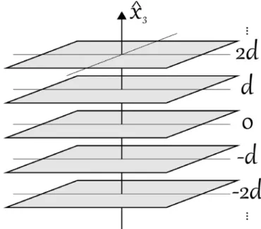
− <d x3<d, as shown inFigs. 1and2, respectively. Basically they

differ on their treatment of the sign provided byx x3/| |3, above and below the corresponding region. The solution that applies to

<x <d

0 3 takes into account that ⎡ ⎣ ⎢ ⎛ ⎝ ⎜ ⎞ ⎠ ⎟⎤ ⎦ ⎥ ⎛ ⎝ ⎜ ⎞ ⎠ ⎟

∑

= − =−∞ +∞ − | − | e

k x d

kd cosh 2 sinh 2 , (41) n

k x nd

3 3 ⎡ ⎣ ⎢ ⎛ ⎝ ⎜ ⎞ ⎠ ⎟⎤ ⎦ ⎥ ⎛ ⎝ ⎜ ⎞ ⎠ ⎟

∑

_| −_{− |} = − =−∞ +∞ − | − | x nd

x nde

k x d

kd sinh 2 sinh 2 , (42) n

k x nd 3

3

3 3

which yield the following multi-layer solution:

⎛ ⎝ ⎜ ⎞ ⎠ ⎟ ⎛ ⎝ ⎜ ⎜ ⎜ ⎜ ⎜ ⎡ ⎣ ⎢ ⎛ ⎝ ⎜ ⎞ ⎠ ⎟⎤ ⎦ ⎥ ⎡ ⎣ ⎢ ⎛ ⎝ ⎜ ⎞ ⎠ ⎟⎤ ⎦ ⎥ ⎞ ⎠ ⎟ ⎟ ⎟ ⎟ ⎟

∑

Ψ= − − → ≠ → → ·→ + c e kd

k x d

ik

k k x

d sinh 2 cosh 2 sinh 2 ₍₄₃₎ k k

i k x

0

3

3

The validity of Eq.(43)is restricted to the region0<x3<d. For the

region shown inFig. 2, namely− <d x3<d, the sum over the layers

consider the x3=0 layer separately, ∑n_≠ e− | − |+e− | | k x nd k x

0 3 3 and

∑ _{≠ (x} −_{nd x/}| −_{nd e}|₎ − | − |+_e− | |_{( /x x}| |₎

n

k x nd k x

0 3 3 3 3 3 3 , to obtain that

⎡ ⎣ ⎢ ⎢ ⎢ ⎛ ⎝ ⎜ ⎜ ⎜ ⎞ ⎠ ⎟ ⎟ ⎟ ⎛ ⎝ ⎜ ⎜ ⎜ ⎞ ⎠ ⎟ ⎟ ⎟ ⎤ ⎦ ⎥ ⎥ ⎥

∑

Ψ= − | | + − → ≠ → → ·→ − | | + ₊

c e e

ik k x x e kx ik k kx 1 2 ( 1) cosh( )

sinh( ) , (44) k

k

i k x k x

kd 0 3 3 3 3 3

In this last expression the single layer solution of Eq. (28) is easily retrieved by taking the limit d→ ∞. To obtain the mean values, similar to the single layer solution, it is required that the mean value be taken over a well-defined unit cell since along the direction perpendicular to the layers l¼d:

∫

d x V3 / ( )⋯ ≡

∫

ddx d d x A/

∫

/ ( )⋯

0 3

2 _{. Then one obtains that} ⎛ ⎝ ⎜ ⎜ ⎞ ⎠ ⎟ ⎟

∫

| | =Ψ

∑

| |

→ ≠ → d x V d c k kd 2 coth 2 , (45) k k 3 2 0 2

∫

d xΨ σ Ψ† =

V 0, (46)

3

1

∫

d xΨ σ Ψ† =

V 0, (47)

3 2 ⎛ ⎝ ⎜ ⎞ ⎠ ⎟

∫

Ψ σ Ψ† =

∑

| |

→ ≠ → d x V c kd sinh 2 , (48) k k 3 3 0 2 2 ⎛ ⎝ ⎜ ⎜ ⎞ ⎠ ⎟ ⎟

∫

∇ | | =Ψ

∑

| |

→ ≠

→

d x

V d k c

kd 8 coth 2 . (49) k k 3 2 2 0 2

In the limitd→ ∞, Eqs.(45), (48) and (49) yield their single layer counterparts, given by Eqs.(35), (38) and (39), respectively. Notice that Eq.(48)is non-zero in contrast with the single layer case. Also Eqs.(46) and (49) have a1/dfactor due to the volume integration, which is also present in Eqs.(36) and (39), as the1/lfactor.

Fig. 1.Pictorial view of a stack of layers separated by a distancedshowing the three-dimensional cell associated to the order parameter solution of Eq.(43).

Fig. 2.Pictorial view of a stack of layers separated by a distancedshowing the three-dimensional cell associated to the order parameter solution of Eq.(44).

5. The broken symmetries

A remarkable difference between the single and the multi-layer solutions is that in the latter case the mean value of the local magnetic _field is non-zero and points perpendicularly to the layers, regardless of the choice of the coef_ficients c→_k, according to Eqs.(19), (46), (47), and (48)

⎛ ⎝ ⎜ ⎞

⎠ ⎟

∫

→ Ψ = − πμ

∑

| | ˆ

→ ≠ → d x V h c kd x

( ) 4

sinh 2 . (50) B k k 3 0 2 2 3

This is a clear consequence of the breaking of the space reversal symmetry in the multi-layer case. Nevertheless the multi-layer solution is derived from thefirst-order equations, defined by Eqs. (18) and (19), which do not break this symmetry. Therefore another solution is expected such that the two possible ways of breaking the space reversal symmetry must be possible. Indeed this other solutionΨ′is obtained by expressing Eq.(26)as ψ′ = ψ

| | ′

−

ik k

x

x . (51)

u d

3

3

The corresponding single layer solution is

⎛ ⎝ ⎜ ⎜⎜ ⎞ ⎠ ⎟ ⎟⎟

∑

Ψ′ = ˜ | |

→ ≠

→ − | | →·→ −

c e e i

k k x x 1 (52) k k

k x i k x

0

3

3 3

and the multi-layer is

⎛ ⎝ ⎜ ⎞ ⎠ ⎟ ⎛ ⎝ ⎜ ⎜ ⎜ ⎜ ⎜ ⎡ ⎣ ⎢ ⎛ ⎝ ⎜ ⎞ ⎠ ⎟⎤ ⎦ ⎥ ⎡ ⎣ ⎢ ⎛ ⎝ ⎜ ⎞ ⎠ ⎟⎤ ⎦ ⎥ ⎞ ⎠ ⎟ ⎟ ⎟ ⎟ ⎟

∑

Ψ′ = ˜

− − − → ≠ → → ·→ − c e kd ik

k k x

d

k x d

sinh 2 sinh 2 cosh 2 ₍₅₃₎ k k

i k x

0

3

3

The mean values are given by

⎛ ⎝ ⎜ ⎜ ⎞ ⎠ ⎟ ⎟

∫

| ′| =Ψ

∑

|˜ |

→ ≠ → d x V d c k kd 2 coth 2 , (54) k k 3 2 0 2

∫

d xΨ σ Ψ′† ′ =

V 0, (55)

3

1

∫

d xΨ σ Ψ′† ′ =

V 0, (56)

3 2 ⎛ ⎝ ⎜ ⎞ ⎠ ⎟

∫

Ψ σ Ψ′† ′ = −

∑

|˜ |

→ ≠ → d x V c kd sinh 2 , (57) k k 3 3 0 2 2 ⎛ ⎝ ⎜ ⎜ ⎞ ⎠ ⎟ ⎟

∫

∇ | ′| =Ψ

∑

|˜ |

→ ≠

→

d x

V d k c

kd 8 coth 2 . (58) k k 3 2 2 0 2

The mean local magneticfield is found to point oppositely to the solution used in Eq.(50)

⎛ ⎝ ⎜ ⎞

⎠ ⎟

∫

→ Ψ′ = πμ

∑

|˜ | ˆ

→ ≠ → d x V h c kd x

( ) 4

sinh 2 . (59) B k k 3 0 2 2 3

The existence of solutions with

∫

(d x V h3 / )→_{in opposite directions,}

given by Eqs.(43) and (53), in case of multi-layers is suggestive of the coexistence of these solutions separated by domain walls.

Their free energy has the same form

= ⎛ ⎝ ⎜ ⎜ ⎞ ⎠ ⎟ ⎟

∑

= | | → ≠ → F md c kd kd 4

2 coth 2 ,

(60) k k 2 2 0 2

as obtained from Eqs.(22), (49) and (58). The reverted magnetic field solution has|c→|

k

2_{replaced by} |˜ |c→

k

2_{in the above expression. In} case that|˜ | = |c→_k c→_k|these two solutions are degenerate in energy and favor the onset of domain walls. We will not treat such coexistence here and concentrate our study only in theΨ solution. A remarkable feature of the present approach is the existence of two kinds of supercurrent densities, namely volumetric and superficial, located between layers and within the layers, respec-tively. The single layer results forΨ σ Ψ†1 andΨ σ Ψ†1 , given by Eqs. (29), show that above and below thex3=0layer such valuesflip

sign because of the factorx x3/| |3. Consequently Eq.(19)shows that the magneticfieldsh1andh2, parallel to this layer, are discontin-uous across thex3=0layer. It is a straightforward consequence of

Maxwell's boundary condition that there is a superficial super-current con_figuration given by

⎡ ⎣⎢

⎤ ⎦⎥

ˆ

x × →h + −→h − = π→

c J

(0 ) (0 ) 4 .

(61) sup

3

These boundary conditions under afixed→J_supreveal the mechan-ism of time reversal and parity breaking. The time reversal symmetry transformation is given by→h → −→h in Eq.(61), which is not invariant under this transformation. The parity symmetry transformation, given by

ˆ

x3→ −

ˆ

x3in Eq.(61), is also not invariant. Only the product of the time reversal and parity transformations (PT) remains invariant under the presence of the surface super-current. We_find that the surface supercurrent leads to the onset of a charge density wave whose properties will be studied elsewhere.

6. The angular momentum states

The layered structure has a preferable direction, defined by the x3axis, an so, we take from the total angular momentum

= =_σ

→

=→× ∇ + →

J x

i 2 , (62)

the componentJ3to determine the coefficientsc→_k. It happens that up to order

ε

3 _{Eq. (18) becomes}

σ Ψ

→·∇→ =0 and it holds that σ

→·∇→ =

J

[ ,_i ] 0, i¼1,2,3. Therefore we study J₃Ψ, which is also a solution since →·∇σ →(J₃Ψ)=0. Although we are not treating a quantum mechanical problem here, the present Hilbert space considerations are useful since the order parameter can be regarded as a superposition of angular momentum statesm

=⎛ ⎝ ⎜⎜ ⎞ ⎠ ⎟⎟

∑

Ψ= α Ψ where JΨ = m+ 1 Ψ

2 , ₍₆₃₎

m

m m 3 m m

where

α

mare arbitrary coefficients. For simplicity we shall not study here admixtures and only puremstates, which means that all but one of the coef_ficients

α

m vanish. Consider the orbital angular momentum component l3=x p1 2−x p2 1, which admits a position representation,p_i=( / )( /= i ∂ ∂xi), and also a wave number

representation, xi= ∂ ∂i( / ki) and pi==ki. For instance, apply the

position space representation,l x3( ), to the up component

ψ

uof Eq.

(28): = ⎜⎛ ⎟

⎝

⎞ ⎠

ψ = ∑→ → − →·→− | |

l x( ) _u( )x _kc_k x k x k ei k x k x

space representation it holds thatlψ_u= ∑→ →_k c k 3 ⎡ ⎣⎢ ⎤ ⎦⎥ −_{l k e( )} i k x→·→− | |k x =

3 3 ⎡ ⎣⎢ ⎤ ⎦⎥ ∑→ → → ·→− | | l k c( ) e

k k

i k x k x

3 3 the last expression follows since a sum over a total derivative is null. Thusl3can be thought of as directly acting on the coef_ficients c→_k. In wave number space the eigenvector eigenvalue problem for the l3 operator is easily soluble:

=

= ±

± ±

l km m km

3 , thus ( )k±m and ±=m are the sought eigenstates

and eigenvalues, respectively. For any two functions, fand g, in wave number space, it holds that l f k g k3[ ( ) ( )]=[l f k g k3 ( )] ( )+

f k l g k( )[3 ( )]. For instance,l k3( )= 2

=

+ −

l k k3( ) 0. There are two sets

of eigenvectors of J3: c→_k =ε

(

k k_±/

)

m. The normalization 1/km is introduced to avoid growth of the coefficientsc→_k for largek, and the multiplicative constant

ε

is arbitrary. The total angular momentum eigenvector problem becomes, J3Ψm,±==(±m+

Ψ _± ) m 1

2 , , but the property − = +

−

k k k k

( / )m ( / )m _{shows that there is}

truly just one set of eigenvectors,Ψm≡Ψm,+, since Ψm,−=Ψ−m,+,

as long as m ranges from positive to negative values. Writing ϕ

=

± ±

k ke i gives thatc→_k =εe im± ϕand shows that the two signs, ±m, are associated to rotations in opposite directions by angles

ϕ

±m . Therefore the order parameters become

⎛ ⎝ ⎜ ⎞ ⎠ ⎟ _⎛ ⎝ ⎜ ⎞ ⎠ ⎟ ⎛ ⎝ ⎜ ⎜ ⎜ ⎜ ⎛ ⎝ ⎜ ⎞ ⎠ ⎟ ⎞ ⎠ ⎟ ⎟ ⎟ ⎟

∑

Ψ =ε

→ ≠ + → ·→ + k k e kd kx ik k kx sinh 2

cosh ( )

sinh ,

(64) m

k

m _{i k x}

0

3

3

wherex3=x3−d/2. Interestingly the mean values for the angular

momentum order parameter,

Ψ

m, are independent of m, since ε

|c→_k| =2 2

⎛ ⎝ ⎜ ⎜ ⎞ ⎠ ⎟ ⎟

∫

|Ψ | =ε

∑

→ ≠

d x

V d k

kd 2 1 coth 2 , (65) m k 3 2 2 0

∫

d xΨ σ Ψ† =

V m m 0, (66)

3

1

∫

d xΨ σ Ψ† =

V m m 0, (67)

3 2 ⎛ ⎝ ⎜ ⎞ ⎠ ⎟

∫

Ψ σ Ψ† =ε

∑

→ ≠ d x V kd 1 sinh 2 , (68) m m k 3 3 2 0 2 ⎛ ⎝ ⎜ ⎜ ⎞ ⎠ ⎟ ⎟

∫

∇ |Ψ | =ε

∑

→ ≠

d x

V d k

kd 8 coth 2 . (69) m k 3

2 2 2

0

We_find quite remarkable that the mean magnetic_field, which relies on Eq.(19), and the above Eqs.(66)–(68), is angular momentum (m)

independent. The same holds for the free energy which defines the normal state gap, given by Eqs. (22) and (69), also shown to be m independent. The single layer limit with de_finite angular momentummis simply retrieved from the above equations at the limit d→ ∞ once noticed that the behavior1/d is just a consequence of the volumeV=Ad, and so, in case of the single layer, dcan be replaced by an arbitrary lengthl. We shall not treat here admixtures of differentmstates and concentrate only in the pure cases.

7. The tetragonal lattice

To reach further understanding of the order parameter we simplify matters by restricting the Fourier components, defined as

≡

k1 g n1 1, k2≡g n2 2 (g1=2 / ,π L g1 2=2 /πL2) for a orthorhombic cell =

A L L1 2, to a small set n1= −1, 0, 1 and n2= −1, 0, 1 with

= =

n1 n2 0excluded (no homogeneous state). Then the sum over

→

k is restricted to the eight points ofFig. 3. We shall also restrict our analysis to the tetragonal symmetry which means that

= =

L1 L2 L andg1=g2=g=2 /πL and in this case unit cell A=L 2

will be interpreted as that of the checkerboard pattern. Then the order parameter becomes

Eq.(70)describes the multi-layer order parameter with restricted Fourier components in a well-defined angular momentum state, as defined byJ3whose eigenvalues are given by Eq.(63). Because of the restricted Fourier space it has the property thatΨm+8=Ψm.

Again we notice that mean values acquire very simple forms, which aremindependent

⎡ ⎣ ⎢ ⎢ ⎛ ⎝ ⎜ ⎞ ⎠ ⎟ ⎛ ⎝ ⎜ ⎞ ⎠ ⎟ ⎤ ⎦ ⎥ ⎥

∫

d x|Ψ | =ε +

V gd

gd gd

4 2 coth

2 2 coth

2

2 , ₍₇₁₎

m 3

2 2

∫

d xΨ σ Ψ† =

V m m 0, (72)

3

1

∫

d xΨ σ Ψ† =

V m m 0, (73)

3 2 ⎡ ⎣ ⎢ ⎢ ⎢ ⎢ ⎢ ⎛ ⎝ ⎜ ⎞ ⎠ ⎟ ⎛ ⎝ ⎜ ⎞ ⎠ ⎟ ⎤ ⎦ ⎥ ⎥ ⎥ ⎥ ⎥

∫

d xΨ σ Ψ† =ε +

V 4 gd gd

1 sinh 2 1 sinh 2 2 , (74) m m 3 3 2 2 2 ⎜ ⎟ ⎜ ⎟ ⎜ ⎟ ⎜ ⎟ ⎛ ⎝ ⎜ ⎞ ⎠ ⎟ ⎛ ⎝ ⎜ ⎜ ⎜ ⎜ ⎡ ⎣⎢ ⎛ ⎝ ⎞ ⎠ ⎛ ⎝ ⎞ ⎠ ⎤ ⎦⎥ ⎛ ⎝ ⎜ ⎞ ⎠ ⎟ ⎡ ⎣⎢ ⎛ ⎝ ⎞ ⎠ ⎛ ⎝ ⎞ ⎠ ⎤ ⎦⎥ ⎛ ⎝ ⎜ ⎞ ⎠ ⎟ ⎞ ⎠ ⎟ ⎟ ⎟ ⎟ ⎛ ⎝ ⎜ ⎞ ⎠ ⎟ ⎛ ⎝ ⎜ ⎜ ⎜ ⎜ ⎧ ⎨ ⎩ ⎡ ⎣⎢ ⎤ ⎦⎥ ⎡ ⎣⎢ ⎤ ⎦⎥ ⎫ ⎬ ⎭ ⎛ ⎝ ⎜ ⎞ ⎠ ⎟ ⎧ ⎨ ⎩ ⎡ ⎣⎢ ⎤ ⎦⎥ ⎡ ⎣⎢ ⎤ ⎦⎥ ⎫ ⎬ ⎭ ⎛ ⎝ ⎜ ⎞ ⎠ ⎟ ⎞ ⎠ ⎟ ⎟ ⎟ ⎟ Ψ ε π π π π ε π π π π = − + + − − + + + − + + + + − + − + + + + π π π π π π − − − − gd

e m gx m gx gx

e m gx i m gx gx

gd

e m g x x e m g x x gx

e m g x x e m g x x gx

2

sinh 2

cos

2 cos 2 cosh

sin

2 sin 2 sinh

2

sinh 2

cos

2 ( ) cos 2 ( ) cosh 2

sin

2 ( ) sin 2 ( ) sinh 2

,

(70) m

i m

m

i m i m

i m i m

( /2)

1 2 3

( /2)

1 2 3

( /2)

1 2 ( /4) 1 2 3

((( 1) )/4)

1 2 ((( 1) )/4) 1 2 3

⎡

⎣ ⎢ ⎢

⎛

⎝ ⎜ ⎞

⎠

⎟ ⎛

⎝

⎜ ⎞

⎠ ⎟ ⎤

⎦ ⎥ ⎥

∫

d x∇ |Ψ | =ε + V

g d

gd gd

32 2 coth

2 2 coth

2

2 . ₍₇₅₎

m 3

2 2 2

They are straightforwardly obtained from Eqs. (65)–(69), once noticed that there are four identical contributions coming from→k along the axis and other four coming from the diagonals ofFig. 3, and each set contributes withk¼gandk= 2g, respectively.

8. The experimental values

We show here that the normal (above the homogeneous) state gap can be determined by assumption of the experimental value for the local magneticfield between layers. To completely deter-mine the multi-layer order parameter, given by Eq. (70), the constant

ε

must be obtained. This indefiniteness is also present in the free energy obtained from Eqs.(22) and (69).

= ⎡

⎣

⎢ ⎛

⎝ ⎜ ⎞

⎠

⎟ ⎛

⎝ ⎜ ⎞

⎠ ⎟⎤

⎦ ⎥ ε

= +

F m

g

d coth

gd

coth gd

4 32

2

2 2 2 . (76)

2 2

The so-called infrared limit, or limit of very small wave number, of the above expression shows undoubtedly the existence of a normal state gap density

= ε → ∞ →

F L d

m

( ) 48 ( / ) .

(77)

2 2

As previously discussed, the constant

ε

is determined by small magnetic _field condition set by experimental limit of NMR/NQR [15,16]andμSR[17,18]experiments. To establish this connection between theory and experiment we obtain the mean value of the local magnetic _field from Eq. (19). Interestingly for a

Ψ

m state

∫

(d x V h3/ )→=0_{for a single layer while for a stack of layers} ⎡

⎣ ⎢ ⎢ ⎢ ⎢ ⎢

⎛ ⎝ ⎜ ⎞

⎠

⎟ ⎛

⎝

⎜ ⎞

⎠ ⎟ ⎤

⎦ ⎥ ⎥ ⎥ ⎥ ⎥

∫

πμ ε

π π

→

= − + ˆ

β d x

V h d

L

d L

x

16 1

sinh

1

sinh 2

.

(78) 3

2

2 2

3

The vanishing of the meanfield for a single layer but not for multi-layers is a consequence of a“solenoid”effect. The meanfield of the single supercurrent loop vanishes but for a stack of current loops it does not vanish, since it is non-zero inside and zero outside. Because Eq.(78)applies for anymthis solenoid interpretation is not directly related to circulating supercurrents within the layers. Next we take that this experimental threshold sets the theoretical mean value

∫

d x→ =

V h hexp, ₍₇₉₎

3

where we choose to work with hexp₌0.01Gauss. The ratio d L/

must also be known to determine the value of

ε

, wheredis the distance between two consecutive layers andLde_fines the size of the tetragonal unit cell within a layer. For numerical purposes we have in mind the compound YBa Cu O2 3 7 0.08₋ as this material presents the checkerboard pattern [27] withL=4a=1.6 nm, as we takea¼0.4 nm andd¼1.2 nm. Thus this ratio is given by

= d

L 0.75. (80)

In convenient units the Bohr magneton isμ_B=9.2 Gauss nm3, and then we obtain the numerical value of

ε

2

ε2=_5.3×₁₀−4_{nm .}−3 (81)

Finally we obtain the free energy, which is the normal state gap

= −

F 0.5 meV nm .3 (82)

For comparison we give the approximate values for the super-conducting gap density of metals and cuprates. They are

− −

104meV nm 3and 10 meV nm 3_{, respectively. This follows from} the BCS formulaFgap= Δ2 ng, where2Δis the energy required to

break a single Cooper pair and ng represents the density of available Cooper pairs, namely ng=0.187Δn E/ F, n and EF being

the electronic density and the Fermi energy, respectively, for metals_n∼_{0.1 nm}−3_,

Δ_/E ∼₁₀−

F 4and2Δ∼1.0 meV, while for the

cuprates the gap is 10 times larger than that of metals, Δ∼

2 10 meV, and ng ∼1.0 nm−

3

, since there are a few Cooper pairs [28] occupying the coherence length volume, ξ ξab c2 , where

ξab∼1.5 nm,ξc∼0.3 nm. In the next section we show that the

stability of this inhomogeneous state is due to topology, which prevents its decay into the lower energy homogeneous state (F¼0).

9. The topological charge

The order parameter

Ψ

mdescribes a lattice of skyrmions and to understand its topological properties we invoke the Moebius strip, formed by rotating one end of 180°and joining it with the other end. Once glued in this way it cannot be returned to the 0° con_figuration. This introduces a discrete number which counts the number of twists present in the Moebius strip. In case of the skyrmions the number of skyrmion cores within a layer plays the role of the twists in the Moebius strip.Figs. 4–6show these skyrmion cores because superficial supercurrents circulate around them. The skyrmion cores are sinkholes and at the same sources of magneticfield stream lines that cross the layer. These streamlines form closed loops around a given layer, which is then perforated twice. The condition that→∇·→h =0cannot be violated makes the rupture of these streamline loops nearly impossible, the fact that brings stability to the

Ψ

mskyrmion solution. Thus similar to the twists in the Moebius strip, the closed loops of magnetic field streamlines cannot be made disappear in favor of a no loop

a

b

c

d

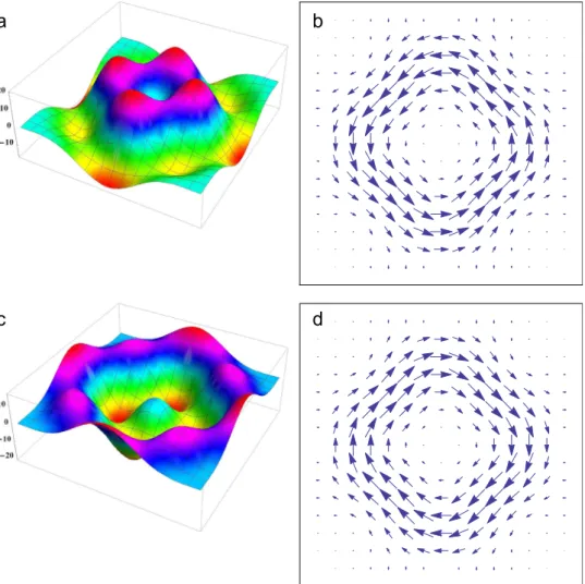
Fig. 5.The subplots (a) and (c) show the local magneticfield,h3, and the subplots (b) and (d) the surface supercurrent,Js, for theJ3=3/2= and J3= −3/2= states, respectively.

a

b

c

d

Fig. 4.The subplots (a) and (c) show the local magneticfield,h3, and the subplots (b) and (d) the surface supercurrent,Js, for theJ3=1/2= and J3= −1/2= states, respectively.

configuration. From a mathematical perspective the topological stability stems from the existence of two closed surfaces that can be mapped one into the other, namely a torus into a sphere. The torus is a consequence of the lattice pattern since the unit cell has periodic boundary conditions. The sphere is a consequence of the global rotational symmetrySU(2)of the order parameter that can be identi_fied with anS2-sphere. The mapping of the torus into the sphere defines the second homotopy group ofS2_,Π

=

S Z

( )

2 2

, which is the topological charge, or skyrmionic number. Thus the integerZ defines the number of possible magnetic field configurations around a layer, which is ultimately de_fined by the number of cores. This is the skyrmion's topological charge and is given by the following expression:

⎡

⎣ ⎢ ⎢ ⎛

⎝

⎜⎜ ⎞

⎠ ⎟⎟

⎤

⎦ ⎥ ⎥

∫

π

= ∂ ˆ

∂ × ∂ ˆ ∂ · ˆ

=

d x h

x h

x h

Q 1

4 ,

(83) x

2

1 2

0 3

wherehˆ =→h h/|→|. The topological charge is not invariant under the time reversal symmetry operation →h → −→h. We find that this skyrmionic topological charge is a function of the angular mo-mentumm, as shown inTable 1.Table 1becomes cyclic form>3, which means the statem¼0 has the same topological charge of

them¼4 state, the statem¼1 has the same charge of them¼5

state and so on. To calculate the topological chargeQwe integrate numerically Eq.(83)using the software Mathematica. Wefind an

upper bound limit to the existence of the topological with regard to the unit cell size, calledLmax, but not a lower bound limit. The checkerboard pattern L¼1.6 nm falls within this limit, L<L_max.

SurprisinglyLmaxfor the casem¼0 is different from the remaining ones, and there are skyrmions only in the range1.2≲d L/ < ∞, whereas for the remaining it holds that0.01<d L/ < ∞.

Fig. 6.The subplots (a) and (c) show the local magneticfield,h3, and the subplots (b) and (d) the surface supercurrent,Js, for the J3=5/2= and J3= −5/2=states, respectively.

Table 1

Limits of the skyrmionic charge for the eigenvectorsΨm,_±.

m Ψm

Q d

Lmax

J3

4 þ1 0.01 ₋7₌

2

3 þ2 0.01 ₋5₌

2

2 2 0.01 ₋3₌

2

1 1 0.01 ₋1₌

2

0 þ1 1.2 ₊1₌

2

þ1 þ2 0.01 ₊3₌

2

þ2 2 0.01 ₊5₌

2

þ3 1 0.01 ₊7₌

A remarkable property of the present model is that the mean magnetic field value taken in any two-dimensional unit cell parallel to the layer at0<x3<dis

⎡

⎣ ⎢ ⎢ ⎢ ⎢ ⎢

⎛ ⎝ ⎜ ⎞

⎠

⎟ ⎛

⎝

⎜ ⎞

⎠ ⎟ ⎤

⎦ ⎥ ⎥ ⎥ ⎥ ⎥

∫

πμ ε

π π

→

= − _β + ˆ

d x

A h d

L

d L

x

16 1

sinh

1

sinh 2

.

(84) x

2

2

2 2

3 3

exactly as given in Eq.(78).

Further understanding of the present model is brought by Figs. 4–6. They contain plots that are all obtained from the order parameter

Ψ

m, given by Eq.(70). Themstates are also called by theirJ3values, namely,=(m+1)

2 , according to Eq.(63). The cases =

= ±

J₃ 1

2 (m¼0 andm¼ 1),± = 3

2 (m¼1 and m¼ 2), and± = 5 2 (m¼2 and m¼ 3) are shown inFigs. 4_–6, respectively. Each of

thesefigures contains four plots associated to the sameJ3modulus, two for the positiveJ3state, and the other two for the negativeJ3 state. The surface supercurrent →J_s and the local magnetic _field componenth3are shown along a selected layer. The surface super-current is shown through arrows that indicate its circulation within the layer and the h3 three-dimensional plot has the interesting feature of having positive and negative values, confirming the presence of magnetic _filed stream lines crossing the layer. Thus the subplots of Figs. 4–6 correspond to the following. Subplots (a) and (b) displayh3andJsfor themstate, respectively, whereas subplots (c) and (d) are associated to theh3 andJs−m−1state, respectively. Comparison between subplots (b) and (d) for each of these three _figures show that the surface supercurrents for the cases m and −m−1are the reverse of each other. Comparison between subplots (a) and (c) indicate an apparent reversal ofh3sign for all the threefigures. In fact this reversal does not exist because subplots (a) and (c) must have the same mean value given by Eq. (68). They do have the same mean magnetic_field sign (negative) determined by Eq.(78). Therefore it is quite remarkable thatFigs. 4–

6display subplots with both senses of angular momentum, which means surface supercurrents circulating in opposite senses and yet the mean magneticfield points in one single direction for all cases. We look in more details each one of the_figures. Subplots (a) and (b) of Fig. 4 describe the J₃= 1₂= (m=0) state. Indeed periodic boundary conditions show that each corner carry one-fourth of the circulation of a single skyrmion at the unit cell in agreement with Table 1that gives, for this case, thatQ=+1. The corner of the unit cell hash3<0and is where the skyrmion core is located. Subplots

(c) and (d) of Fig. 4 describe the J₃= − 1₂= state, whose super-current circulation is just in the opposite direction, andQ= −1. The h3plot is not the reverse of the previous case, as it seems to be, since both have the same value of

_∫

(d x A h2/ ) 3. Subplots (a) and (b) ofFig. 5describe the J₃= 3=

2 (m=1)state. Nevertheless in this case near to the corner there two skyrmions instead, and according toTable 1Q=+2. The corner of the unit cell hash3<0and is where

the skyrmion core is located. Subplots (c) and (d) ofFig. 4describe the J₃= − 1₂= state, whose supercurrent circulation is just in the opposite direction andQ= −2.Fig. 6shows circulation around the center of the unit cell in the opposite direction of previousfigures. Subplots (a) and (b) ofFig. 6describe the J₃= 5=

2 (m=2) state. According toTable 1Q= −2. Subplots (c) and (d) ofFig. 4describe the J₃= − 1₂= state, whose supercurrent circulation is just in the opposite direction andQ=+2.

10. Conclusions

We show here that a very simple theoretical framework upholds properties to describe a topological state that we con-jecture to be the pseudogap. To account for this the theory must contain at least two order parameters. We have studied the angular momentum properties of this state and calculated the gap that separates it from the homogeneous state under the condition that the local magnetic_field falls below the threshold set by NMR/NQR andμSRexperiments. This inhomogeneous state is a lattice of skyrmions that breaks time reversal symmetry and leads to the checkerboard pattern.

Acknowledgments

The authors thank Edinardo Ivison Batista Rodrigues for allow-ing the use ofFigs. 1and2from his master thesis entitled“The Lichnerowicz-Weitzenböck formula applied to superconductors with one and two-components”. Mauro M. Doria and Alfredo. A. Vargas-Paredes acknowledge the Brazilian agency CNPq, Facepe and Inmetro forfinancial support.

References

[1]J. Bednorz, K. Müller, Z. Phys. B: Condens. Matter 64 (2) (1986) 189. [2]H. Alloul, T. Ohno, P. Mendels, Phys. Rev. Lett. 63 (1989) 1700.

[3]A. Shekhter, B.J. Ramshaw, R. Liang, W.N. Hardy, D.A. Bonn, F.F. Balakirev, R. D. McDonald, J.B. Betts, S.C. Riggs, A. Migliori, Nature 498 (2013) 75. [4]S. Kaminski, A. Rosenkranz, H.M. Fretwell, J.C. Campuzano, Z. Li, H. Raffy, W.

G. Cullen, H. You, C.G. Olson, C.M. Varma, H. Hochst, Nature 416 (2002) 610. [5]J. Xia, E. Schemm, G. Deutscher, S.A. Kivelson, D.A. Bonn, W.N. Hardy, R. Liang,

W. Siemons, G. Koster, M.M. Fejer, A. Kapitulnik, Phys. Rev. Lett. 100 (2008) 127002.

[6]R.-H. He, M. Hashimoto, H. Karapetyan, J.D. Koralek, J.P. Hinton, J.P. Testaud, V. Nathan, Y. Yoshida, H. Yao, K. Tanaka, W. Meevasana, R.G. Moore, D.H. Lu, S.-K. Mo, M. Ishikado, H. Eisaki, Z. Hussain, T.P. Devereaux, S.A. Kivelson, J. Orenstein, A. Kapitulnik, Z.-X. Shen, Science 331 (6024) (2011) 1579. [7]H. Karapetyan, M. Hücker, G.D. Gu, J.M. Tranquada, M.M. Fejer, J. Xia,

A. Kapitulnik, Phys. Rev. Lett. 109 (2012) 147001.

[8]J.E. Hoffman, E.W. Hudson, K.M. Lang, V. Madhavan, H. Eisaki, S. Uchida, J. C. Davis, Science 295 (5554) (2002) 466.

[9]M. Vershinin, S. Misra, S. Ono, Y. Abe, Y. Ando, A. Yazdani, Science 303 (5666) (2004) 1995.

[10]K. McElroy, D.-H. Lee, J.E. Hoffman, K.M. Lang, J. Lee, E.W. Hudson, H. Eisaki, S. Uchida, J.C. Davis, Phys. Rev. Lett. 94 (2005) 197005.

[11]J.-X. Li, C.-Q. Wu, D.-H. Lee, Phys. Rev. B 74 (2006) 184515.

[12]G. Ghiringhelli, M. Le Tacon, M. Minola, S. Blanco-Canosa, C. Mazzoli, N. B. Brookes, G.M. De Luca, A. Frano, D.G. Hawthorn, F. He, T. Loew, M.M. Sala, D. C. Peets, M. Salluzzo, E. Schierle, R. Sutarto, G.A. Sawatzky, E. Weschke, B. Keimer, L. Braicovich, Science 337 (6096) (2012) 821.

[13]B. Fauqué, Y. Sidis, V. Hinkov, S. Pailhès, C.T. Lin, X. Chaud, P. Bourges, Phys. Rev. Lett. 96 (2006) 197001.

[14]Y. Li, et al., Phys. Rev. B 84 (2011) 224508.

[15]S. Strässle, J. Roos, M. Mali, H. Keller, T. Ohno, Phys. Rev. Lett. 101 (2008) 237001. [16]S. Strässle, B. Graneli, M. Mali, J. Roos, H. Keller, Phys. Rev. Lett. 106 (2011) 097003. [17]G.J. MacDougall, A.A. Aczel, J.P. Carlo, T. Ito, J. Rodriguez, P.L. Russo, Y.J. Uemura,

S. Wakimoto, G.M. Luke, Phys. Rev. Lett. 101 (2008) 017001.

[18]J.E. Sonier, V. Pacradouni, S.A. Sabok-Sayr, W.N. Hardy, D.A. Bonn, R. Liang, H. A. Mook, Phys. Rev. Lett. 103 (2009) 167002.

[19]C.M. Varma, Phys. Rev. B 73 (2006) 155113. [20]P. Bourges, Y. Sidis, C. R. Phys. 12 (2011) 461.

[21]M. Cariglia, A.A. Vargas-Paredes, M.M. Doria, Europhys. Lett. 105 (3) (2014) 31002.

[22]G.E. Volovik, L.P. Gor'kov, Sov. Phys. JETP 61 (1985) 843.

[23]M.M. Doria, A.R.C. de Romaguera, F.M. Peeters, Europhys. Lett. 92 (1) (2010) 17004.

[24]M.M. Doria, A.A. Vargas-Paredes, J.A. Helayel-Neto, Modern Phys. Lett. B 26 (11) (2012) 1230005.

[25]A.A. Vargas-Paredes, M.M. Doria, J.A.H. Neto, J. Math. Phys. 54 (1) (2013) 013101.

[26]P.A. Marchetti, F. Ye, Z.B. Su, L. Yu, Europhys. Lett. 93 (5) (2011) 57008. [27]Z. Islam, X. Liu, S.K. Sinha, J.C. Lang, S.C. Moss, D. Haskel, G. Srajer, P. Wochner,

D.R. Lee, D.R. Haeffner, U. Welp, Phys. Rev. Lett. 93 (2004) 157008. [28]B. Batlogg, Phys. Today 44 (6) (1991) 44.