Rev. Bras. Econ. vol.66 número3

(1)

Finance Premium of Public Non-Financial

Corporations in Brazil

Fernando N. de Oliveira

∗

, Alberto Ronchi Neto

†

Contents: 1. Introdução; 2. Theoretical Background; 3. Data; 4. Empirical Analysis; 5. Robustness Analysis; 6. Conclusion.

Keywords: Monetary Transmission Mechanism; Credit Channel; Balance Sheet Channel. JEL Code: G30, G32

Our objective in this paper is to analyze empirically the relationship between the external finance premium of non-financial corporations in Brazil with their default probability and with their demand for inven-tories. As for the former relation, we find that corporations that have greater external finance premium have greater probability of default. As for the latter, we find that the external finance premium is positive and statistically significantly correlated. The results confirm previous results of the literature that indicate that the balance sheet channel of monetary policy is relevant in Brazil.

Nosso objetivo nesse trabalho é analisar empiricamente como o prêmio de financiamento externo de empresas não-financeiras no Brasil se relaciona com a probabilidade de default e com o nível de estoques. No primeiro exercí-cio, as empresas com maior prêmio de financiamento externo apresentaram uma maior probabilidade de default. Com relação ao segundo exercício, o prêmio de financiamento externo apresentou uma correlação positiva e es-tatisticamente significante com o nível de estoques. A análise confirmou resultados anteriores da literatura que indicam que o canal do balanço pat-rimonial da política monetária é relevante para o Brasil.

1. INTRODUÇÃO

In Brazil, the credit channel is a recent phenomenon. The high inflation before the Real Plan pre-vented credit market’s development. Even after the economy reached price stability, the real interest rate high volatility and the internal and external shocks that were commonplace in Brazil dampened

∗_{Central Bank of Brazil Research Department Rio de Janeiro and Assistant Professor IBMEC/RJ. E-mail:}_{fernando.nascimento@} bcb.gov.br

(2)

this process. Over the last years, however, the gradual removal of some factors that used to make the country susceptible to these shocks allowed the interest rate reductions and the credit supply expan-sion. In this context, the credit channel grows in importance.

The credit channel’s theory enhances how credit market imperfections amplify monetary policy effects. In this framework, the external finance premium is the key variable, defined as the difference between the cost of raising funds externally and the opportunity cost of internal funds. However, as Graeve (2008) depicts, a major problem for empirical studies in this area is that the external finance premium is unobservable.

In this way, great part of empirical work that tries to test this monetary transmission mechanism set proxies to external finance premium and verifies differences in business cycle responses and corporate investments between groups of firms separated according to constraints faced in credit market access. Gertler and Gilchrist (1994) and Oliveira (2009), for example, used financial indicators to reflect the external finance premium dynamic and the firm size to measure the credit market access, focusing on firms from United States and Brazil respectively. Both papers show that small firms have a more sensitive business cycle to changes in external finance premium. This result is considered an evidence of credit channel working in these economies.

In this paper, we use financial indicators usually related with credit market imperfections to show the existence of common factors between the external finance premium and the firm’s default prob-ability and study the sensitivity of business cycle, represented by inventories, to the external finance premium.

Our database comes from Economática and Comissão Valores Mobiliários (CVM). Our database con-sist of a unbalanced panel data formed with information of non-financial publicly held companies listed at Bovespa from the third quarter of 1994 to third quarter of 2009. Insolvency and global long-term debt rating were the criteria that we chose to measure the firm’s credit market access. The concept of insol-vency adopted was the beginning of a bankruptcy or recovery legal procedure. This information was obtained from Bovespa’s Daily Information Bulletin (Boletim Diário de Informações – BDI) and CVM’s publicly held companies register. The rating’s information was obtained in Fitch Ratings, Moodys and Standard & Poors release list. The sample consists of 332 firms, of which 12 are insolvent firms and 37 are firms with ratings for its long-term debt.

Considering that companies that became insolvent through time must have faced more constraints in credit market access, the default probability must be directly proportional to external finance pre-mium. Using Logit and Complementary Log Log regressions to relate a dummy variable created for the insolvent companies and indicators related with the external finance premium, we have obtained evidence supporting this hypothesis.

We selected our credit constrained sample based on our credit restriction criteria and used this sample to relate firm’s inventories and the external finance premium, by estimating a dynamic panel data model System GMM. Our results showed that:

(1) the credit channel in Brazil gained strength after the introduction of primary fiscal surplus, inflation targets and free-floating exchange rate in 1999;

(2) insolvent and no rating firms have the inventories more elastic to the external finance premium;

(3) firms with financing operations directly obtained at the BNDES have inventories less sensitive to the external finance premium; and

(4) economic sectors often highlighted as formed by firms with small scale, history of financial prob-lems and high level of external and unfair competition showed more elasticity of inventories to the external finance premium.

(3)

finance premium and default probability. In the second one, our identification of credit market restric-tions using the insolvency criteria is also original.1

The rest of the paper is structured as follows. Section 2 reviews existing literature focusing on the description of credit channel theory and characteristics often designed to measure credit market access. Section 3 provides data description. Section 4 presents the empirical work. Section 5 does robustness analysis. Section 6 concludes.

2. THEORETICAL BACKGROUND

Following Bernanke and Gertler (1995), there are two mechanisms connecting monetary shocks and the external finance premium. The first one, the bank-lending channel, emphasizes how monetary policy affects bank’s credit supply. The second one, the balance sheet channel, explores the mone-tary policy impacts over borrower’s balance sheet. These mechanisms are broadly called as the credit channel.

In bank lending channel, a monetary contraction causes a decrease in demand deposits, reducing the bank’s loans supply. Even if this reduction doesn’t imply a total restriction to credit costs associated with the establishment of relationships and capture of resources with new lenders would increase the agency costs in loan contracts and raise the external finance premium. Considering that bank deposits do not have a perfect substitute, the capital replacement by banks would generate additional costs that also could raise the external finance premium. In turn, the higher external finance premium would decrease the credit demand, the investment’s level and the economic growth level.

In the balance sheet channel, a tighten monetary policy would affect adversely the firm’s financial position at least in three ways:

(1) reduces the asset prices, diminishing the value of collateral available as guarantee for new and actual loans;

(2) raises the interest expenses, decreasing the company’s cash flow; and

(3) decreases the consumption level, affecting profits and impacting the company’s cash flow again.

The firm’s deteriorated balance sheet raises the counterparty risk for lenders and scrutinizes new credit contracts. Moreover, the reduction in firms net worth increases the moral hazard involved in companies’ management once the owners share value is lower, encouraging riskier investments. This movement raises the external finance premium and restricts the credit supply, the investments level and the aggregate demand.

According to Mishkin (1995), between these mechanisms, the balance sheet channel has been high-lighted by its background theory rationality. Among the elements that stand this mechanism out are the further rationale for asset price effects emphasized in monetarist thinking and the fact that unlike the traditional view in the monetary policy transmission is the short term nominal interest rate, not the long term real interest rate, which drives the monetary shocks effects to real economy.

Great part of empirical works found in literature tries to gauge at the existence of an active credit channel through the balance sheet channel background. The usual way tries to obtain proofs about the financial accelerator importance to corporative sector distinguishing the behavior of business cycle and investment decisions between different groups of firms separated according to financial constraints faced in credit market access.

Gertler and Gilchrist (1994) follow this strategy appraising the importance of financial factors over a non-financial group of firms in United States. This study used firm’s size measured through the

1_{As for the debt ratings as a criterion to measure the credit market access, Gilchrist and HimmelberG (1995), Gilchrist (1998)}

(4)

total assets as the criteria to indicate the firm’s credit market access. They chose four firm’s financial indicators to analyze: inventories, sales, short-term debt and coverage ratio.2 _{The sales level take into} account nonfinancial factors related to changes on demand. The inventories levels are set to explain effects related to credit market frictions that forbids firms to smooth production when sales decline. The short-term debt considers the financing structure role on credit market access. The coverage ratio is a proxy to firm’s overall financial positions. After some empirical exercises, Gertler and Gilchrist conclude that balance sheet effects can be more relevant form smaller firms.

Oliveira (2009) undertakes a similar work as Gertler and Gilchrist (1994) adopting the firm’s size as a measure of credit market access. This study concentrates on Brazil’s economy. The empirical analysis was conducted over a database of public and private firms firms between the third quarter of 1994 and the third quarter of 2007. One point to emphasize in this article is the addition of some factors in order to describe firm’s characteristics related to another agency costs. Besides the usual variables linked to nonfinancial and financial issues (operational revenues, inventories, short term debt and coverage ratio), the ratio of market value to the book value (Market to Book) and the ratio of fixed assets to total assets are considered to capture firm’s growth capacity and level of collateral respectively. Following Gertler and Gilchrist (1994), Oliveira (2009) indicate that smaller firms are more sensitive to balance sheet effects.

Gilchrist and HimmelberG (1995), Gilchrist (1998) investigate the influence of fundamental (expected return and present value) and financial (availability of internal and external funds) factors on firms investment decisions considering capital market imperfections. Among others characteristics, the au-thors adopted the existence of debt rating as a criterion to measure the credit market imperfections. According to the authors, considering that most companies that issues public debt obtains a bond rat-ing, this strategy permits to split the sample into firms that have, or not, issued public debt in the past. If the company didn’t issue debt it must have faced more constraints in credit market access. Their empirical analyses indicated that non- rating firms are more sensitive to financial factors.

3. DATA

Our data comes from Economática and CVM. We had originally collected balance sheet information of 628 non-financial publicly held companies from third quarter of 1994 to third quarter of 2009.

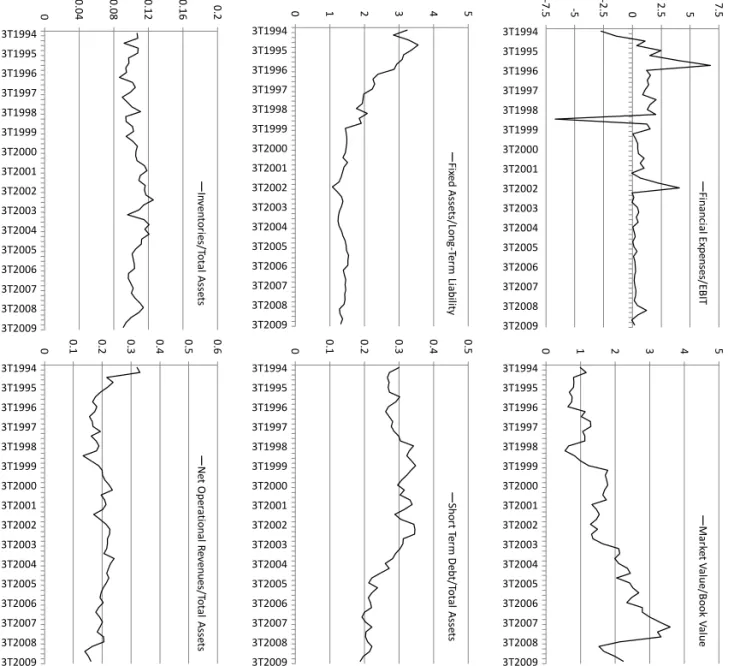
For each company, we build the following ratios: Financial Expenses/EBIT,3Market Value/Book Value, Fixed Assets/Long-Term Liability, Short Term Debt/Total Assets, Net Operational Revenues/Total Assets, and Inventories/Total Assets. The ratios Financial Expenses/EBIT and Short Term Debt/Total Assets aim to control for firm’s financial position and debt structure respectively. The ratios Market Value/Book Value and Fixed Assets/Long-Term Liability are set to express agency costs. These four financial indica-tors were used as a proxy to the external finance premium. The ratios Net Operational Revenues/Total Assets and Inventories/Total Assets were used to obtain a robust business cycle measure over both financial and non financial factors.

We chose the insolvency and global long-term debt rating as the criterions to measure firm’s credit market access. The concept of insolvency adopted was the beginning of a bankruptcy or recovery legal procedures. This information was obtained from Bovespa’s Daily Information Bulletin (Boletim Diário de Informações - BDI) and CVM’s publicly held companies register. We defined the default moment the quarter when the firm appeared asconcordatária4_{in BDI or bankrupted in CVM’s register. We called} theses firms “insolvents”. We created a dummy variable equal to one if the company was insolvent and

2_{The ratio of cash flow to total interest payments.}

3_{Earnings before interest and taxes.}

4_{This is the term in Brazilian Business Recovery Law for companies that have opened a recovery legal procedure due to}

(5)

zero otherwise. The assumption is that firms that became insolvent would have face greater agency costs through time.

The debt rated firms were identified at Fitch Ratings, Moodys and Standard & Poors release list. We created a dummy variable for this criteria assigning the value one if the firm has a rating for its long term debt released at least in two of the three credit rating agencies and zero otherwise. Considering that firms with rating have access to a greater number of funding sources, these companies must be less sensitive to credit market imperfections.

We exclude from our sample:

(1) companies that didn’t have in any quarter available information to calculate the indicators selected for the analysis;

(2) companies from financial sectors (banks, insurance companies, etc.), that have a very different fi-nancing structure comparing to non financial companies; and

(3) companies that belong to Telecommunication and Electric Energy sectors, that in Brazil are tradi-tionally characterized by a strong resilience of business cycle at times of crises.

Table 1 shows a summary statistics to the total sample and the sample separated according to insolvency and rating criterions. Panel A of Table 1 shows the existence of outliers into the data. In order to avoid problems we also excluded from the sample 0.2 percentile from all indicators. Panel B of Table 1 displays the data description after the outliers’ exclusion.

After all exclusions, we obtained an unbalanced panel covering 332 firms. Of these, we identified 12 insolvent and 37 with rating. Table 2 indicates the amount of firms found in each criterion as well the sector it is part of. We adopted Economática’s sector classification. Table 3 presents the indicators correlation matrix. With the exception of the correlation observed between the ratios Net Operational Revenues/Total Assets and Inventories/Total Assets, all the correlations were below 0.1.

Tables 4 and 5 reveal the test’s results to appraise the difference between the indicators averages accordingly with the criterions adopted to measure the firm’s credit market access. Comparing solvent and insolvent firms, considering a 10% significance level, the tests indicated that the averages of the ra-tios Financial Expenses/EBIT, Short Term Debt/Total Assets, Net Operational Revenues/Total Assets, and Inventories/Total Assets for insolvent firms are superior to the averages for the solvent ones. Contrary to this result, the averages of the ratios Market Value/Book Value and Fixed Assets/Long-Term Liability for solvent firms are superior to the averages obtained for the insolvent ones. All this results are as expected.

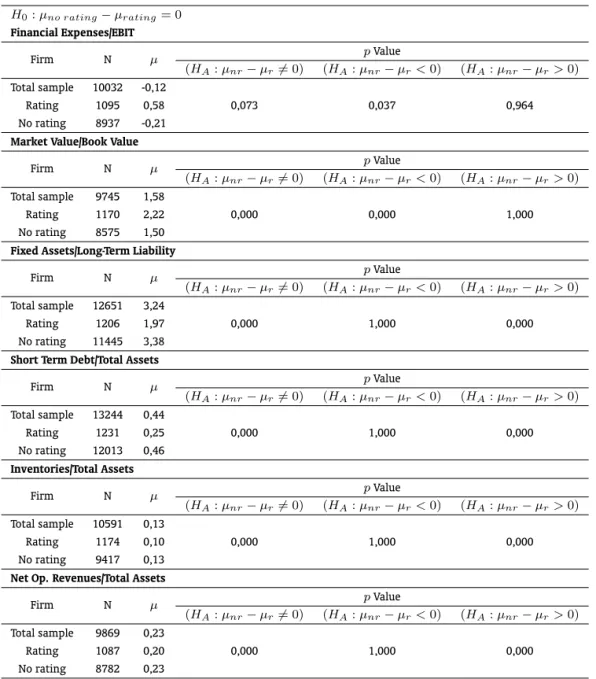
Considering the rating criterion, the tests indicated that the average of the ratios Fixed Assets/Long-Term Liability, Inventories/Total Assets, Short Assets/Long-Term Debt/Total Assets, and Net Operational Revenues/Total Assets for firms without rating are superior to the averages obtained for the ones with rating. In the case of the ratios Financial Expenses/EBIT and Market Value/Book Value the averages for the firms with rating are superior to the average obtained for the ones without rating. Although the results found for the ratios Fixed Assets/Long-Term Liability and Financial Expenses/EBIT were unlike the expected, they can be minimized considering that the medians for firms with and without rating are very similar.5

Due to the small amount of insolvent companies in our sample we employed the Kaplan Meier estimator as a non-parametric test to confirm the parametric tests results.6_{Figure 2 displays the result} of Kaplan Meier estimator to the total sample. Figure 3 contains the result of Kaplan Meier estimator splitting the sample between solvent and insolvent firms.

The results of this test show that the probability for companies to go from solvent to insolvent state decreases as times goes by. This dynamic demonstrates the greater insolvency probability expected for

5_{This can be observed in Table 1.}

(6)

younger companies, which in turn poses one of the primitive factors related to firm’s credit market access commented by Gertler and Gilchrist (1994).7 _{As a second result, the Kaplan Meier estimator} between insolvent firms is very different from the measure obtained for the solvent firms and total sample.

4. EMPIRICAL ANALYSIS

4.1. The relationship between the external finance premium and the default

prob-ability

According to credit channel’s theory there is an inversely proportional relationship between the firm’s financial position and the external finance premium. Furthermore, many researchers have demon-strated that commonly used indicators to denote the firm’s balance sheet condition has predictive power to identify the credit risk in corporative sector.8 _{These relationships suggest the existence of} common factors between the external finance premium and the firm’s default probability.

In order to test this hypothesis we applied the non-linear probability models Logit and Complemen-tary Log Log to relate the insolvency dummy variable and the indicators selected to denote the credit market imperfections. The result of this exercise could present favorable evidences to the use of insol-vency as a criterion to measure credit market access and confirm the indicators selected to denote the external finance premium dynamic.

The Logit regression is the commonly used technique in bankruptcy prediction, presenting advan-tages over others techniques.9_{In order for its implementation, the dependent variable suffers a logistic} transformation, been converted in an odds ratio and after in a log base variable.10 _{Our Logit model has} the following form:

ln

p

1−p

=β0+β1i+β2f ee+β3mb+β4cl+β5std+v (1)

where

i = The ratio Inventories/Total Assets, in order to denote business cycle dynamics;

f ee = The ratio Financial Expenses/EBIT (the inverse of coverage ratio), in order to control for firms financial position;

mb = The ratio Market Value/Book Value (Market to Book), in order to control to the growth potential that the market attributes for companies;

cl = The ratio Fixed Assets/Long-Term Liability, in order to control for the level of collateral available as a guarantee for new and actual loans;

std = The ratio Short Term Debt/Total Assets, in order to control for the firm’s financing structure;

v = random error component.

7_{Gertler and Gilchrist (1994) enhance that the informational frictions that affects the external finance premium apply mainly to}

younger firms, firms with a high degree of idiosyncratic risk, and firms that are not well collateralized. They justify the use of the firm’s size criterion to split their sample of companies asserting that the firm’s size is strong correlated with this three “primitive factors”.

8_{Sanvincente and Minardi (1998) and Brito and Assaf Neto (2008) are some of the papers that presented researches that used}

some indicators usually related to credit market imperfections to bankruptcy prediction in Brazil.

9_{Brito and Assaf Neto (2008).}

(7)

According to Cameron and Trivedi (2005), the Complementary Log Log regression is more appro-priate when one of the outcomes is rare.11 _{This technique assumes an asymmetric distribution for} the random error component. In order for its implementation the dependent variable also suffers a transformation, been converted in a set of exponential terms and after in a log base variable.12 _Our Complementary Log Log model has the following form:

ln(−ln(1−p)) =β0+β1i+β2f ee+β3mb+β4cl+β5std+v (2)

We estimated the equations as a pool of cross sections and allowing for intragroup correlation in standard errors (cluster robust standard errors). Table 6 displays the estimated coefficients for the Logit and Complementary Log Log regressions. The results were very similar. With the exception of the ratio Fixed Assets/Long-Term Liability, both models presented all variables significant at 10% level. Under credit channel’s background, all the coefficients revealed the expected signal.

The coefficients of the ratios Market Value/Book Value and Fixed Assets/Long Term Liability have a negative signal. This indicates that the higher the value of this indicators, the smaller the default probability. The coefficients of the ratios Financial Expenses/EBIT, Short Term Debt/Total Assets, and Inventories/Total Assets have a positive signal. This indicates that the higher the value of this indica-tors, the higher the default probability. Among all the independent variables the ratio Inventories/Total Assets presented the higher coefficient.

Figures 4 and 6 display these relationships in a clearly way. For each indicator we calculated the default’s conditional probability keeping the others equal to the average. In others words, the figures presents the default’s conditional probability for a representative firm with an average value for all the indicators except the one that is emphasized. For each indicator the probabilities obtained from both Logit and Complementary Log Log model can be compared.

4.2. Inventories and the external finance premium

In order to appraise the relationship between inventories and the external finance premium we employed the two stage dynamic panel data model developed by Arellano and Bover (1995) and Blun-dell and Bond (1998), also known as System GMM. This method is an extension of the Arellano-Bond estimator.13

The System GMM combines the original equation at first differences from Arellano-Bond estimator with an equation at levels in a system of equations and employs both lagged levels and differences as instruments. This strategy permits to solve problems that arise in Arellano-Bond estimator when instruments are weakly correlated with the independent variables.14

11_{Typically, the Logit regression is more accurate to measure marginal effects and obtain probability prediction when the analyzed}

events have a proportion close to1

2. Considering that in our final sample we have identified just 12 insolvent firms against 320

solvent firms, providing 92 insolvency events against 6690 solvency events, the application of this technique for comparing effects is recommended.

12_{The Complementary Log Log transformation has the form:}_{P r}₍_d_{= 1}_/X_{) = 1}₋_exp₍₋_exp₍_Xβ₎₎_{. For small values of}

probability, the Complementary Log Log transformation is close to the logistic transformation. As this probability increases, the transformation approaches infinity more slowly than logistic transformation.

13_{Holtz-Eakin et al. (1988) and Arellano and Bond (1991) developed the Arellano-Bond estimator, also known as Difference GMM.}

14_{A recognized and widespread fact in dynamic panel data models’ literature is that the larger the series persistence, the lower}

(8)

We chose the ratio Inventories/Total Assets to denote the corporative business cycle variable. We es-timated a first order univariate process (AR(1)) for this variable using the total sample (1994Q3-2009Q3) and we obtained a coefficient for the autoregressive term around 0.3, demonstrating some persistence degree in this ratio.15 _{This result implies that the first difference of the ratio Inventories/Total} As-sets must present a lower correlation with the lags in level, what could result in weak instruments’ problems. In our exercise, the time dimension couldn’t be considered small, reducing the risk of bias. Nevertheless, we believe that using System GMM we can at least obtain an efficiency gain. The next equation presents our base model:

Ii,t=β0+β1Ii,t−1+β2N ORi,t+β3F EEi,t−1+

β4M Bi,t−1+β5CLi,t−1+δ6ST Di,t−1+ηi+vit (3)

where:

Ii,t = The ratio Inventories/Total Assets, in order to denote business cycle dynamics;

N ORi,t = The ratio Net Operational Revenues/Total Assets, in order to control for non financial factors that could explain differences in firms with different levels of credit market access;16

F EEi,t = The ratio Financial Expenses/EBIT (the inverse of coverage ratio), in order to control for firms financial position. This is our balance sheet variable;

M Bi,t = The ratio Market Value/Book Value (Market to Book), in order to control to the growth poten-tial that the market attributes for companies;

CLi,t = The ratio Fixed Assets/Long-Term Liability, in order to control for the level of collateral avail-able as a guarantee for new and actual loans;

ST Di,t = The ratio Short Term Debt/Total Assets, in order to control for the firm’s financing structure;

ηi = firm’s fixed effect;

vit = random error component.

We avoided seasonality problems considering all variables as changes over the same quarter of the past year. In order to remove universal time related shocks from the errors we included time dummies in the model.17 All the specifications were estimated with robust and Windmeijer correction for standard

lower the correlation between the first difference of this series and the lag of levels. In turn, the use of weak instruments affects the performance of the Arellano-Bond estimator in large and small samples. In large samples, the variance of the estimated coefficients increases asymptotically. In small samples, particularly when the time dimension is reduced, the use of weak instruments may provide bias in coefficients. The System GMM supposes additional assumptions to Arellano-Bond estimator, like the inexistence of correlation between the first difference of instrumental variables and the fixed effects. This assumption allows the use of more instruments, providing estimation advantages comparing with its precursor. Bobba and Coviello (2006) and Biondi and Toneto JR. (2008) enhances this points originally raised by Blundell and Bond (1998). Roodman (2009) provides a revision of GMM dynamic panel data model and shows how to implement these estimators with Stata.

15_{These results weren’t presented entirely due to space limitations, but we can provide this information at request.}

16_{Gertler and Gilchrist (1994) enhance that non financial factors, such as contracting out and others industry effects, could}

explain changes in firm’s business cycle. In this way, including controls for these non financial factors would provide a better measure of variations in firm’s business cycle due to financial factors.

17_{According to Roodman (2009), the inclusion of time dummies make more likely the assumption that the errors are not correlated}

(9)

errors. The model is subject to the following assumptions:E(vit) =E(vit×ηi) =E(vit×vjS) = 0

for alli,j,t,s,i6=j.

Besides the lag of the ratio Inventories/Total Assets, we also treat the ratio Net Operational Rev-enues/Total Assets as a predetermined variable. In this way, in order to validate the System GMM instruments, the following additional moment conditions must be satisfied:

E(Ii,t₋1∆vit) = 0, for all t = 3, . . . , T; E(∆Ii,t−1(ηi +vit)) = 0, for all t = 4, . . . ,T;

E(N ORi,t₋1∆vit) = 0 for all t = 2, . . . , T; andE(∆N ORi,t−1(ηi +vit)) = 0for all t = 3,

. . . ,T; where∆denotes the first difference operator. This identification strategy permits some advan-tages. Allowing these weak exogeneity assumptions the inventories can be viewed as a forward-looking variable that takes into account the expected level of inventories and demand.

Besides the “internal instruments”,18 we also include time dummies and the short term nominal interest rate (Selic) as instruments. In order to avoid the instrument proliferation, the instruments were limited to two lags.19

Table 7 displays the estimated parameters. The Hansen test has as null hypothesis the validity of the instruments. The Difference-in-Hansen test has as null hypothesis the validity of the additional System GMM moment conditions. Both tests don’t reject the null hypothesis.20 _{Considering a 90%} confidence level, the ratios Net Operational Revenues/Total Assets, Market Value/Book Value and Fixed Assets/Long-Term Liability didn’t present statistically significant coefficients.

The lag of the ratio Inventories/Total Assets presented a significant coefficient with a value between zero and one (0.339). This result indicates that the firm’s inventories level follows a stationary process and demonstrates persistence in its dynamic.

The ratios Financial Expenses/EBIT and Short Term Debt/Total Assets also presented significant co-efficients with positive signal. The higher these ratios, the higher the sensitiveness of business cycle measured by the dynamics of inventories.

The others indicators didn’t present coefficient statistically significant.

4.3. The corporative business cycle sensitiveness according to firm’s credit

mar-ket access

We analyzed the corporative business cycle sensitiveness accordingly to firm’s credit market access, measured by insolvency and global long-term debt rating. Firms that face more constraints in credit market access must demonstrate greater sensitiveness to balance sheet effects. In order to test this hypothesis we created the following dummies variables:

• D: dummy variable equal to one if the firm have became insolvent during the period and zero otherwise;

• r: dummy variable equal to one if the firm obtained a rating for its long term debt and zero otherwise.

For each criterion we built a specification of the base model presented in last section including an interaction term obtained from the cross product between the dummies variable and the indicators related to credit market access. We are interested in the significance and signal of these interaction terms and indicators. The equations (4) and (5) denote these specifications:

18_{The lagged levels and the lagged differences from the predetermined variables.}

19_{According to Cameron and Trivedi (2005), for moderate or large time dimension there may be a maximum lag of the dependent}

variable that is used as an instrument, such as not more than its fourth lag.

20_{Both tests Hansen and Difference-in-Hansen lose confidence as the number of instruments increases. However, we did these}

(10)

Ii,t=δ0+δ1Ii,t−1+δ2N OR+i,t+δ3F EEi,t−1+δ4(D∗F EEi,t−1)

+δ5M Bi,t−1+δ6(D∗M Bi,t−1) +δ7CLi,t−1+δ8(D∗CLi,t−1)+

δ9ST Di,t−1+δ10(D∗ST Di,t−1) +ηi+vit (4)

Ii,t=δ0+δ1Ii,t−1+δ2N OR+i,t+δ3F EEi,t−1+δ4(D∗F EEi,t−1)+

δ5M Bi,t−1+δ6(r∗M Bi,t−1) +δ7CLi,t−1+δ8(r∗CLi,t−1)+

δ9ST Di,t−1+δ10(r∗ST Di,t−1) +ηi+vit (5)

The specifications were estimated just for the period following the economic policy tripod estab-lishment.

Considering the specification (4), that includes a dummy variable equal to one for insolvent firms, we expect that the interaction term present the same signal of the respective indicator. Regarding the specification (5), that includes a dummy variable equal to one for debt rate firms, we expect that the interaction term present the opposite signal of the respective indicator. We will take these results as evidences of balance sheet effects, which amplify the monetary policy shocks over corporative business cycle.

Table 9 reveals the estimated parameters. All the indicators coefficients kept the significance and signal observed in base model. In order to appraise the significance of the interaction term and re-spective indicator, besides the individual significance test, we also applied the Wald test to assess the jointly significance of the variables. Tables 10 and 11 summarize the tests results and coefficients of these variables.

We classified the coefficients according to significance and signal obtained. The coefficients that presented individual or joint significance with the expected signal were classified as “valid” (V). The coefficients that presented individual or joint significance with signal against our expectation were classified as “not valid” (NV). The coefficients that didn’t present individual or joint significance were classified as “not conclusive” (NC).

In the specification considering the insolvency criterion, we obtained valid results for the ratios Financial Expenses/EBIT and Fixed Assets/Long-Term Liability. The ratio Market Value/Book Value pre-sented a not conclusive result. The ratio Short Term Debt/Total Assets prepre-sented a not valid result. In the specification considering the rating criterion, the ratios Fixed Assets/Long-Term Liability and Short Term Debt/Total Assets presented valid results. The other ratios presented not conclusive results. Except for the ratio Market Value/Book Value, all the ratios presented at least one valid result at the adopted criterions.

5. ROBUSTNESS ANALYSIS

In order to appraise the dynamic panel data model that we have presented in last section, we conducted four experiments in this section:

1. We estimated the model preceding and following the economic policy “tripod” establishment in Brazil, based on primary fiscal surplus, inflation targets and free-floating exchange rate. This period consider the sample after the fourth quarter of 1999;

2. We analyzed the “‘BNDES” effect;

(11)

The specifications constructed in order to appraise these experiments are presented next. They followed the same assumptions and instruments’ rule choice assumed in base model.

5.1. The relationship between the corporative business cycle and the external

fi-nance premium preceding and following the establishment of the economic

policy “tripod” in Brazil

We estimated the base model preceding and following the economic policy “tripod” establishment in Brazil, based on primary fiscal surplus, inflation targets and free-floating exchange rate. This issue is important for credit channel, once the monetary policy suffered significant changes after this event. Ta-ble 8 displays the results for both specifications. The only significant variaTa-bles in the period preceding the tripod establishment were the lag of the dependent variable and the ratio Net Operational Rev-enues/Total Assets. The coefficients of indicators introduced to denote the external finance premium weren’t significant. In the period following the tripod establishment, considering a 90% confidence level, only the ratio Net Operational Revenues/Total Assets didn’t present a significant coefficient. The coefficients of all ratios related with external finance premium were significant and presented signal as expected. We interpreted this result as evidence that the credit channel gained strength after the tripod establishment.

5.2. The “BNDES effect” analysis

A particular feature about Brazil’s credit market is the involvement of BNDES (The Brazilian Devel-opment Bank). This institution is a key player in the implementation of government’s industrial policy and the main long term financing provider. The funds offered by BNDES have better cost and maturity conditions compared with other financing agents from Brazil’s credit market. Furthermore, the long term interest rate charged for funds obtained in the development bank21_{are just marginally affected by} the short term interest rate that Central Bank controls. In such a context, firms that have more access to BNDES funds must present more resilience to external finance premium variation. In order to evaluate this hypothesis we used the same method applied in last subsection. We collected available informa-tion about BNDES’s direct operainforma-tions and identified in our sample the firms that obtained finance lines for large-scale investment projects in the institution. Table 12 reveals these companies according to its sector. We used this information to create the following dummy variable:

• BNDES: dummy variable equal to one if the firm obtained finance line for large-scale investments and zero otherwise.

The equation (6) denotes a model specification including the interaction term calculated as the cross product between the dummy variable and the indicators related to balance sheet effects:

Ii,t=γ0+γ1Ii,t−1+γ2N ORi,t+γ3F EEi,t−1+γ4(BN DES∗F EEi,t−1)+

γ5M Bi,t−1+γ6(BN DES∗M Bi,t−1) +γ7CLi,t−1+γ8(BN DES∗CLi,t−1)+

γ9ST Di,t−1+γ10(BN DES∗ST Di,t−1) +ηi+vit (6)

Once again, we are interested in the significance and signal of the interaction terms and respective indicators. Due to the rule considered in the dummy variable creation, we expect that the interaction terms present the opposite signal revealed by the indicators. This result would indicate that firms in our

(12)

sample that obtained funds with BNDES to finance large-scale investments presented more resilience to credit market imperfections.

Table 13 shows the estimated parameters. We also estimated this specification for the period after the tripod establishment in Brazil. Comparing these results with the ones that we obtained in the base model estimation, the ratio Financial Expenses/EBIT was the only indicator that lost significance.

Table 14 summarizes the coefficients and significance tests for the indicators related to credit market imperfections. We classified the indicators following the same rule applied in the experiment from the last subsection: the coefficients that presented individual or joint significance with the expected signal were classified as “valid” (V). The coefficients that presented individual or joint significance with signal against our expectation were classified as “not valid” (NV). The coefficients that didn’t present individual or joint significance were classified as “not conclusive” (NC).

While the ratio Financial Expenses/EBIT didn’t present individual significance, the Wald test pointed that the indicator and its interaction term are jointly significant. With this result, we considered the ratio Financial Expenses/EBIT as valid. We also obtained a valid result for the ratio Fixed Assets/Long-Term Liability. The others ratios presented not conclusive results.

5.3. The sector’s corporative business cycle sensitiveness

After the identification of a credit channel working, the discussions must be addressed to micro issues. In such context the knowledge about how the different sectors in economy behave facing credit market imperfections grows in importance for monetary and industrial policies. In order to contribute with this issue, in this subsection we intend to rank the sectors accordingly with the sensitiveness to the external finance premium.

Our sample represents 15 sectors: agriculture and fisheries, foods and beverages, retail, construc-tion, electro-electronics, industrial machinery, mining, non-metallic minerals, pulp and paper, oil and gas, chemical, metallurgy and steelmaking, textile, transportation, and vehicles and spare parts. Fol-lowing the methodology applied in last subsections, we calculated interaction terms crossing a dummy variable created for each sector in our sample with the indicators related to the credit market imperfec-tions.

In order to obtain the sector’s sensitiveness we estimated one specification for each sector. We kept the same indicators and instruments in all specifications to provide comparable results. The equation (7) denotes the general specification:

Ii,t=γ0+γ1Ii,t−1+γ2N ORi,t+γ3F EEi,t−1+

γ4(S∗F EEi,t−1) +γ5M Bi,t−1+γ6(S∗M Bi,t−1) +γ7CLi,t−1+

γ8(S∗CLi,t−1) +γ9ST Di,t−1+γ10(S∗ST Di,t−1) +ηi+vit (7)

The dummy sector is represented in equation with the term “S”. After we evaluate the coefficient’s significance of the indicator and interaction terms, we added the coefficients if they were individu-ally or jointly significant (“valid” - V) and disregard if they didn’t present significant coefficients (“not conclusive” - NC).

Due to space restrictions, we opted to expose just the coefficients indicators related to credit market imperfections and interaction terms for each sector’s specification.22 _{Summarizing the results that we} didn’t present, in all specifications the coefficient of the ratio Inventories/Total Assets have kept the significance, positive signal and value between zero and one. The ratio Net Operational Revenues/Total assets remained not significant. The Hansen and Difference-in-Hansen tests have continued to indicate the validity of instruments and System GMM moments conditions.

(13)

Tables 15 to 18 denote the estimated parameters for the ratios Financial Expenses/EBIT, Market Value/Book Value, Fixed Assets/Long-Term Liability, and Short Term Debt/Total Assets. Tables 19 and 20 reveal for each indicator the sector’s ranking classification according to the total marginal effect obtained adding the coefficients of the indicator itself and respective interaction term.

The sector that appeared in more ranks with positive sensitiveness was the textile, with three in-dicators (Market Value/Book Value, Fixed Assets/Long-Term Liability, and Short Term Debt/Total Assets). The sectors that appeared two times were foods and beverages (Financial Expenses/EBIT and Short Term Debt/Total Assets), chemical (Financial Expenses/EBIT and Market Value/Book Value), transporta-tion (Market Value/Book Value and Fixed Assets/Long-Term Liability), vehicles and spare parts (Fixed Term Liability and Short Term Debt/Total Assets), and paper and pulp (Fixed Assets/Long-Term Liability and Short Assets/Long-Term Debt/Total Assets). The sectors agriculture and fisheries (Financial Ex-penses/EBIT), electro-electronics (Market Value/Book Value), and construction (Fixed Assets/Long-Term Liability) appeared once.

The sectors that appeared in more ranks with negative signal were electro-electronics (Financial Expenses/EBIT and Short Term Debt/Total Assets), construction (Financial Expenses/EBIT and Market Value/Book Value), retail (Market Value/Book Value and Fixed Assets/Long-Term Liability), foods and beverages (Market Value/Book Value and Fixed Assets/Long-Term Liability), and agriculture and fish-eries (Fixed Assets/Long-Term Liability and Short Term Debt/Total Assets). The sectors mining (Fixed Assets/Long-Term Liability), paper and pulp (Financial Expenses/EBIT), and metallurgy and steelmaking (Fixed Assets/Long-Term Liability), appeared just once.

6. CONCLUSION

In this paper we investigated the relationship between the external finance premium and firm’s default probability and appraised in different levels the sensitivity of corporative business cycle to the external finance premium.

Using Logit and Complementary Log Log regressions we found that some commonly indicators used to express the external finance premium present an explanatory power for the firm’s default probability. We interpret this result as evidence supporting the insolvency as a good proxy to credit market access and the external finance premium. This result is important once we didn’t identify the use of this criterion in literature.

We used the System GMM estimator to appraise the relationship between the business cycle and external finance premium. The additional moment conditions that this estimator assumes permits to avoid weak instruments’ problems arising when variables with persistence are employed. Moreover, our identification strategy allowed us to treat inventories as a forward- looking variable considering the expected inventory itself and sales. This strategy avoided us to assume the stronger assumption of exogeneity between inventories and sales.

When we estimated the base model splitting our sample preceding and following the tripod estab-lishment in Brazil, we found results indicating a stronger credit channel after this event. Considering that after this event the Brazilian credit market have developed significantly, assuming a trajectory of reduction for interest rates and expansion in credit volume, this result seems coherent. This also indicates a better effectiveness of monetary policy through credit channel in the more recent period.

(14)

use of these resources for investments must provide a better financial condition and capacity to new investments, easing the balance sheet effects over the firms.

Our analyses using the insolvency and the existence of rating for firm’s long term debt to separate the sample according to the credit market access indicated that insolvent and no rating firms are more sensitive to the external finance premium. Companies that face different levels of constraints in credit market access demonstrate a different response to monetary policy shocks through credit channel.

For us, the results in this paper make it clear as well as confirm previous results in the literature, such as Oliveira (2009), showing that the balance sheet channel is relevant in Brazil to explain the effects of monetary policy on the real sector of the economy.

BIBLIOGRAPHY

Arellano, M. & Bond, S. (1991). Some tests of specification for panel data: Monte Carlo evidence and an application to employment equations. Review of Economic Studies, 58(2):277–297.

Arellano, M. & Bover, O. (1995). Another look at the instrumental-variable estimation of error-components models.Journal of Econometrics, 68(1):29–52.

Bernanke, B. S. & Gertler, M. (1995). Inside the black box: The credit channel of monetary policy trans-mission. Journal of Economic Perspectives, 9(4):3–10.

Bernanke, B. S., Gertler, M., & Gilchrist, S. (1999). The financial accelerator in a quantitative business cycle framework.The Handbook of Macroeconomics, 1(21):1341–1393.

Biondi, R. L. & Toneto JR., R. (2008). Regime de metas inflacionárias: Os impactos sobre o desempenho econômico dos países.Estudos Econômicos, 38(4):873–903.

Blundell, R. & Bond, S. (1998). Initial conditions and moment restrictions in dynamic panel data models. Journal of Econometrics, 87(1):115–143.

Bobba, M. & Coviello, D. (2006). Weak instruments and weak identification in estimating the effects of education on democracy. Working paper n. 569., Inter-American Development Bank (IADB).

Bond, S. (2002). Dynamic panel data models: A guide to micro data methods and practice. Working paper cwp09/02. London, Institute for Fiscal Studies.

Brito, G. A. S. & Assaf Neto, A. (2008). Modelo de classificação de risco de crédito de empresas. Revista Contabilidade & Finanças, 19(46):18–29.

Cameron, A. C. & Trivedi, P. K. (2005). Microeconometrics: Methods and applications. First edition. Cambridge, Cambridge University Press.

Cameron, A. C.; Trivedi, P. K. (2009). Microeconometrics using Stata. Stata Press, College Station. Texas.

Gertler, M. & Gilchrist, S. (1994). Monetary policy, business cycles and the behaviour of small manufac-turing firms.The Quarterly Journal of Economics, 109(2):309–340.

Gilchrist, S.; Himmelberg, C. P. (1998). Investment, fundamentals, and finance. NBER working paper series 6652, National Bureau of Economic Research.

Gilchrist, S. & HimmelberG, C. P. (1995). Evidence on the role of cash flow for investment. Journal of Monetary Economics, 36(3):541–572.

(15)

Hall, S. (2001). Credit channel effects in the monetary transmission mechanism. Winter, Bank of England Quarterly Bulletin.

Holtz-Eakin, D., Newey, W., & Rosen, H. S. (1988). Estimating vector autoregressions with panel data. Econometrica, 56(6):1371–1395.

Hubbard, R. G. (1995). Is there a credit channel for monetary policy? Federal Reserve Bank of St. Louis Review, 77(3):63–77.

Mishkin, F. S. (1995). Symposium on the monetary transmission mechanism. Journal of Economic Per-spectives, 9(4):27–48.

Mishkin, F. S. (1996). The channels of monetary transmission: Lessons for monetary policy. NBER working paper series 5464, National Bureau of Economic Research.

Oliveira, F. N. (2009). Effects of monetary policy on corporations in Brazil: An empirical analysis of the balance sheet channel. Forthcoming, Brazilian Review of Econometrics.

Rajan, R. G. & Zingales, L. (1998). Financial dependence and growth. American Economic Review, 88(3):559–586.

Roodman, D. (2009). How to do xtabond2: An introduction to difference and system GMM in stata. The Stata Journal, 9(1):86–136.

Sanvicente, A. Z.; Minardi, A. (1998). Identificação de indicadores contábeis significativos para a previsão de concordata de empresas. Working paper, Instituto Brasileiro de Mercado de Capitais.

Torabi, M. R. & Ding, K. (1998). Selected measurement and statistical issues in health education evalua-tion and research. The International Electronic Journal of Health Education, 1:26–38.

(16)

Fernando N. de Oliveira e Alberto R onchi Neto Figur e 1: Financial Indicators time series -7

.5 -5 -2.5 0 2.5 5 7.5

3T1994 3T1995 3T1996 3T1997 3T1998 3T1999 3T2000 3T2001 3T2002 3T2003 3T2004 3T2005 3T2006 3T2007 3T2008 3T2009 F in a n ci a l E xp e n se s/ E BI T

0 1 2 3 4 5

3T1994 3T1995 3T1996 3T1997 3T1998 3T1999 3T2000 3T2001 3T2002 3T2003 3T2004 3T2005 3T2006 3T2007 M a rk e t V a lu e /Bo o k V a lu e

0 1 2 3 4 5

3T1994 3T1995 3T1996 3T1997 3T1998 3T1999 3T2000 3T2001 3T2002 3T2003 3T2004 3T2005 3T2006 3T2007 3T2008 3T2009 F ix e d A ss e ts /L o n g -T e rm L ia b ili ty

0 0.1 0.2 0.3 0.4 0.5

3T1994 3T1995 3T1996 3T1997 3T1998 3T1999 3T2000 3T2001 3T2002 3T2003 3T2004 3T2005 3T2006 3T2007 S h o rt Te rm D e b t/ To tal A ss e ts 0 0 .0 4 0 .0 8 0 .1 2 0 .1

6 0.2

3T1994 3T1995 3T1996 3T1997 3T1998 3T1999 3T2000 3T2001 3T2002 3T2003 3T2004 3T2005 3T2006 3T2007 3T2008 3T2009 In v e n to rie s/ To ta l A ss e ts

0 0.1 0.2 0.3 0.4 0.5 0.6

(17)

Table 1: Financial indicator’s descriptive statistics

Panel A: Data description - With outilers

Firms N µ σ min 25% 50% 75% max

Total Sample

Financial Expenses/EBIT 10072 0,60 126,57 -2539 -0,36 0,33 1,15 11321,6 Market Value/Book Value 10976 1,89 14,07 -323,99 0,37 0,85 1,81 985,2 Fixed Assets/Long-Term Liability 14189 6,85 115,56 6,9E-05 0,57 1,31 2,51 8528,8 Short Term Debt/Total Assets 14923 1,53 71,55 3,8E-07 0,19 0,31 0,49 8555,3 Inventories/Total Assets 11974 0,11 0,1 3,3E-06 3,1E-02 9,6E-02 0,17 0,72 Net Op. Revenues/Total Assets 11247 0,22 0,24 -14,02 0,1 0,19 0,28 2,00 Solvents

Financial Expenses/EBIT 9915 0,58 127,56 -2539 -0,35 0,33 1,14 11321,6 Market Value/Book Value 9650 1,79 10,06 -323,99 0,37 0,86 1,84 501,6 Fixed Assets/Long-Term Liability 12500 6,17 88,75 6,9E-05 0,51 1,33 2,6 5349 Short Term Debt/Total Assets 13199 1,68 76,08 3,8E-07 0,2 0,32 0,51 8555,3 Inventories/Total Assets 10441 0,13 9,8E-02 3,3E-06 5,4E-02 1,13E-01 0,18 0,72 Net Op. Revenues/Total Assets 9755 0,23 0,25 -14,02 0,11 0,20 0,30 2,00 Insolvents

Financial Expenses/EBIT 157 1,79 11 -24,16 -0,92 0,38 2,28 88,92 Market Value/Book Value 125 -0,26 5,39 -32,36 -0,42 -5,7E-02 0,5 13,54 Fixed Assets/Long-Term Liability 197 0,94 0,89 7,7E-03 0,22 0,73 1,47 7,18 Short Term Debt/Total Assets 197 0,89 1,51 0,10 0,38 0,58 0,86 13,88 Inventories/Total Assets 183 0,15 0,12 3,13E-04 6,4E-02 9,3E-02 0,24 0,52 Net Op. Revenues/Total Assets 158 0,27 0,22 -0,20 1,3E-01 0,23 0,4 1,05 With rating

Financial Expenses/EBIT 1097 6,16E-01 17,24 -289,25 0,06 0,33 0,95 334,33 Market Value/Book Value 1172 2,17 3,58 -26,42 0,73 1,51 2,78 73,18 Fixed Assets/Long-Term Liability 1206 1,97 5,16 1,7E-03 0,81 1,31 2 138,02 Short Term Debt/Total Assets 1240 0,26 0,30 3,8E-07 0,16 0,23 0,31 9,75 Inventories/Total Assets 1176 0,10 8,3E-02 1,4E-03 4,1E-02 8,4E-02 0,14 0,51 Net Op. Revenues/Total Assets 1087 0,20 0,18 -8,3E-06 0,1 0,17 0,23 1,25 No rating

Financial Expenses/EBIT 8975 5,94E-01 133,95 -3E+03 -4,7E-01 0,33 1,19 11321,6 Market Value/Book Value 8603 1,71 10,59 -323,99 0,33 0,78 1,67 501,59 Fixed Assets/Long-Term Liability 11491 6,52 92,55 6,9E-05 0,46 1,32 2,67 5349 Short Term Debt/Total Assets 12156 1,82 79,28 1,9E-05 0,2 0,34 0,54 8555,29 Inventories/Total Assets 9448 0,13 9,9E-02 3,3E-06 5,7E-02 1,16E-01 0,19 0,72 Net Op. Revenues/Total Assets 8826 0,23 0,25 -1,4E+01 0,11 0,21 0,31 2

(18)

Panel B: Data description - Without outilers∗

Firms N µ σ min 25% 50% 75% max

Total Sample

Financial Expenses/EBIT 10032 -0,12 13,66 -264,1 -0,35 0,33 1,15 145,9 Market Value/Book Value 9745 1,58 3,96 -22,72 0,37 0,85 1,81 73,2 Fixed Assets/Long-Term Liability 12651 3,24 11,32 7,9E-04 0,51 1,32 2,56 385,2 Short Term Debt/Total Assets 13244 0,44 0,54 1,9E-04 0,20 0,32 0,51 7,8 Inventories/Total Assets 10591 0,13 0,10 2,2E-05 5,4E-02 1,12E-01 0,18 0,5 Net Op. Revenues/Total Assets 9869 0,23 0,18 -0,05 0,11 0,20 0,30 1,7 Solvents

Financial Expenses/EBIT 9875 -0,15 13,70 -264,1 -0,34 0,33 1,14 145,9 Market Value/Book Value 9622 1,60 3,96 -22,72 0,38 0,86 1,83 73,18 Fixed Assets/Long-Term Liability 12454 3,28 11,41 7,9E-04 0,51 1,33 2,59 385,2 Short Term Debt/Total Assets 13050 0,43 0,54 1,9E-04 0,20 0,32 0,50 7,8 Inventories/Total Assets 10410 0,13 0,10 2,2E-05 5,4E-02 1,12E-01 0,18 0,48 Net Op. Revenues/Total Assets 9713 0,23 0,18 -0,05 0,11 0,20 0,30 1,72 Insolvents

Financial Expenses/EBIT 157 1,79 11,00 -24,16 -0,92 0,38 2,28 88,92 Market Value/Book Value 123 0,23 3,81 -20,60 -0,42 -4,6E-02 0,50 13,54 Fixed Assets/Long-Term Liability 197 0,94 0,89 7,7E-03 0,22 0,73 1,47 7,18 Short Term Debt/Total Assets 194 0,73 0,67 0,10 0,37 0,57 0,81 5,92 Inventories/Total Assets 181 0,14 0,11 3,1E-04 6,4E-02 9,2E-02 0,24 0,47 Net Op. Revenues/Total Assets 156 0,28 0,21 2,1E-04 0,13 0,23 0,40 1,05 With rating

Financial Expenses/EBIT 1095 5,8E-01 10,92 -208,69 0,06 0,33 0,95 144,40 Market Value/Book Value 1170 2,22 3,40 -13,04 0,73 1,52 2,78 73,18 Fixed Assets/Long-Term Liability 1206 1,97 5,16 1,7E-03 0,81 1,31 2,00 138,02 Short Term Debt/Total Assets 1231 0,25 0,13 3,3E-04 0,17 0,23 0,32 0,88 Inventories/Total Assets 1174 0,10 0,08 1,4E-03 4,1E-02 8,4E-02 0,14 0,44 Net Op. Revenues/Total Assets 1087 0,20 0,18 -8,3E-06 0,10 0,17 0,23 1,25 No rating

Financial Expenses/EBIT 8937 -2,1E-01 13,96 -3E+02 -4,6E-01 0,33 1,18 145,94 Market Value/Book Value 8575 1,50 4,02 -22,72 0,33 0,78 1,66 72,14 Fixed Assets/Long-Term Liability 11445 3,38 11,78 7,9E-04 0,47 1,32 2,66 385,24 Short Term Debt/Total Assets 12013 0,46 0,56 1,9E-04 0,20 0,34 0,53 7,76 Inventories/Total Assets 9417 0,13 0,10 2,2E-05 5,7E-02 1,16E-01 0,19 0,48 Net Op. Revenues/Total Assets 8782 0,23 0,18 -5,3E-02 0,11 0,21 0,31 1,72

∗_{We excluded 0.2 percentiles from the financial indicators.}

(19)

Table 2: Firm’s description according to sectors and credit market access criterion.

Sector Solvents Insolvents With rating Without rating

Foods and beverages 36 1 7 30

Retail 17 0 0 17

Construction 30 0 4 26

Electro-electronics 14 2 0 16

Industrial machinery 7 0 0 7

Mining 6 0 2 4

Non-metallic minerals 3 1 0 4

Pulp and paper 9 0 3 6

Oil and gas 9 0 2 7

Chemical 25 3 3 25

Metallurgy and steelmaking 40 0 6 34

Textile 34 0 1 33

Transportation 14 1 4 11

Vehicles and Spare Parts 21 1 1 21

Agriculture and fisheries 5 0 0 5

Others 50 3 4 49

Total 320 12 37 295

Note:We exclude from our sample: (1) companies that didn‘t have in any quarter available information to calculate the indicators selected for the analysis;

(20)

Table 3: Financial indicators correlation matrix

Market Fixed Short Term Inventories/ Net Op. Expenses/ EBIT Value/Book Assets/Long- Debt/Total Total Revenues/

Value Term Liability Assets Assets Total Assets Financial

1 Expenses/ EBIT

Market Value/

0,0195 1 Book Value

Fixed Assets/

-0,0054 -0,0352 1 Long-Term Liability

Short Term Debt/

-0,0342 -0,0486 -0,0424 1 Total Assets

Inventories/

-0,0115 0,0397 0,0062 0,072 1 Total Assets

Net Op. Revenues/

(21)

Table 4: Equality test of the mean: Solvents x Insolvents

H0:µsolvents−µinsolvents= 0 Financial Expenses/Ebit

Firm N µ pValue

(HA:µs−µi6= 0) (HA:µs−µi<0) (HA:µs−µi>0) Total sample 10032 -0,12

Solvents 9875 -0,15 0,077 0,038 0,962

Insolvents 157 1,79 Market Value/Book Value

Firm N µ pValue

(HA:µs−µi6= 0) (HA:µs−µi<0) (HA:µs−µi>0) Total sample 9745 1,58

Solvents 9622 1,60 0,000 1,000 0,000

Insolvents 123 0,23 Fixed Assets/Long-Term Liability

Firm N µ pValue

Solvents 12454 3,28 0,004 0,998 0,002

Insolvents 197 0,94 Short Term Debt/Total Assets

Firm N µ pValue

Solvents 13050 0,43 0,000 0,000 1,000

Insolvents 194 0,73 Inventories/Total Assets

Firm N µ pValue

Solvents 10410 0,127 0,015 0,007 0,993

Insolvents 181 0,145 Net Op. Revenues/Total Assets

Firm N µ pValue

Solvents 9713 0,228 0,000 0,000 1,000

Insolvents 156 0,278

(22)

Table 5: Equality test of the mean: rating x no rating firms.

H0:µno rating−µrating= 0 Financial Expenses/EBIT

Firm N µ pValue

(HA:µnr−µr6= 0) (HA:µnr−µr<0) (HA:µnr−µr>0) Total sample 10032 -0,12

Rating 1095 0,58 0,073 0,037 0,964

No rating 8937 -0,21 Market Value/Book Value

Firm N µ pValue

(HA:µnr−µr6= 0) (HA:µnr−µr<0) (HA:µnr−µr>0) Total sample 9745 1,58

Rating 1170 2,22 0,000 0,000 1,000

No rating 8575 1,50 Fixed Assets/Long-Term Liability

Firm N µ pValue

Rating 1206 1,97 0,000 1,000 0,000

No rating 11445 3,38 Short Term Debt/Total Assets

Firm N µ pValue

Rating 1231 0,25 0,000 1,000 0,000

No rating 12013 0,46 Inventories/Total Assets

Firm N µ pValue

Rating 1174 0,10 0,000 1,000 0,000

No rating 9417 0,13 Net Op. Revenues/Total Assets

Firm N µ pValue

Rating 1087 0,20 0,000 1,000 0,000

No rating 8782 0,23

(23)

(24)

Figure 3: Kaplan Meier function appraising the default probability to event’s duration between solvent and insolvent firms

Note: Due to the small amount of insolvent companies we employed the Kaplan Meier estimator as a non parametric test to confirm the parametric tests results. According to Torabi and Ding (1998), non parametric tests are indicated in small sample environments. Figure 2 displays the result of Kaplan Meier estimator to the total sample. Figure 3 contains the result of Kaplan Meier estimator splitting the sample between solvent and insolvent firms. The results of this test show that the probability for companies to go from solvent to insolvent state decreases as times goes by. This dynamics

(25)

Table 6: Non linear probability models to appraise the existence of common factors between the exter-nal finance premium and the firm’s default probability

Model Logit Complementary Log Log:

Dependent Variable ln(p/(1−p)) ln(−ln(1−p))

Constant -4,067 -4,037

( 0,000 ) ( 0,000 )

Financial Expenses/EBIT 0,0104 0,010

( 0,024) ( 0,023)

Market Value/Book Value -0,148 -0,132

( 0,011) ( 0,000)

Fixed Assets/Long-Term Liability -0,822 -0,831

( 0,107 ) ( 0,118 )

Short Term Debt/Total Assets 0,336 0,317

( 0,033 ) ( 0,021 )

Inventories/Total Assets 4,934 4,705

( 0,087 ) ( 0,069 )

Wald chi-quadrado(5) 26,43 26,43

Sample 3Q1994 - 3Q2009 3Q1994 - 3Q2009

Note:We estimated the equations as a pool of cross sections and allowing for intragroup correlation in standard errors (cluster robust standard errors). Table 6 displays the estimated coefficients for the Logit and Complementary Log Log regressions. The results were very similar. With the exception f the ratio Fixed Assets/Long-Term Liability, both models present all variables significant o at 10% level. Appraising this result under credit channel’s background, all the coefficients have the expected signal.

(26)

Figure 5: Graphs for the conditional default’s probability evaluated at averages: Fixed Assets/Long-Term Liability and Short Term Debt/Total Assets

0

1

0

.2

0

.4

0

.6

0

.8

-15 -10 -5 0 5

Fixed Assets/Long-Term Liability

Complementary Log Log Logit

0

1

0

.2

0

.4

0

.6

0

.8

0 20 40

Short Term Debt/Total Assets

Figure 6: Graph for the conditional default’s probability evaluated at averages: Inventories/Total Assets

0

1

0

.2

0

.4

0

.6

0

.8

0 1 2 3

Inventories/Total Assets

(27)

Table 7: Base model: dynamic panel data model: studying the relationship between the corporative business cycle and the external finance premium

Dependent Variable Inventories/Total Assets (1)

Constant -0,1120768

(0,000)

Inventories/Total Assets (-1) 0,3388686 (0,002)

Net Op. Revenues/Total Assets -0,0010334 (0,859)

Financial Expenses/EBIT (-1) 0,0000169 (0,007)

Market Value/Book Value (-1) -0,0000779 (0,124)

Fixed Assets/Long-Term Liability (-1) -0,0045212 (0,368)

Short Term Debt/Total Assets (-1) 0,1966661 (0,033)

Hansen (0,184)

Difference-in-Hansen (0,682)

Autocorrelation test A. Bond

(0,004) / (0,402) (1a.order) / (2a.. order)

Total number of instruments 232

Sample n = 248

(28)

Table 8: Base model estimated preceding and following the economic policy “tripod” establishment in Brazil, based on primary fiscal surplus, inflation targets and free-floating exchange rate.

Dependent Variable Inventories/Total Assets

(2) (3)

Constant -0,019 -2,540

(0,722) (0,503)

Inventories/Total Assets (-1) 0,163 0,529

(0,000) (0,000)

Net Op. Revenues/Total Assets 4,76E-01 -6,17E-03

(0,001) (0,392)

Financial Expenses/EBIT (-1) 2,62E-04 2,41E-05

(0,271) (0,085)

Market Value/Book Value (-1) -1,12E-03 -8,92E-05

(0,855) (0,068)

Fixed Assets/Long-Term Liability (-1) 0,045 -0,011

(0,286) (0,040)

Short Term Debt/Total Assets (-1) 0,182 0,186

(0,170) (0,083)

Hansen (0,387) (0,274)

Difference-in-Hansen (0,686) (0,418)

Autocorrelation test A. Bond (0,104) / (0,828) (0,005) / (0,304)

(1a. order) / (2a. order)

Total number of instruments 60 165

Sample n = 70 n = 214

4T94 - 4T98 4T99 - 3T09

(29)

Table 9: Firm’s business cycle sensitiveness according to the credit market access measured through the insolvency and the existence of global rating for the long term debt.

Insolvency Rating

Constant -2,365 -2,667

(0,522) (0,504)

Inventories/Total Assets (-1) 0,527 0,534

(0,000) (0,000)

Net Op. Revenues/Total Assets -6,07E-03 -6,43E-03

(0,395) (0,378)

Financial Expenses/EBIT (-1) 2,41E-05 2,49E-05

(0,082) (0,120)

(Financial Expenses/EBIT) 4,61E-02 -5,75E-05

×Dummy (-1) (0,024) (0,481)

Market Value/Book Value (-1) -8,95E-05 -9,28E-05

(0,066) (0,055)

(Market Value/Book Value) -1,03E-01 -3,26E-02

×Dummy (-1) (0,502) (0,365)

Fixed Assets/Long-Term Liability (-1) -0,011 -0,012

(0,040) (0,018)

(Fixed Assets/Long-Term Liability) -0,437 0,027

×Dummy (-1) (0,225) (0,027)

Short Term Debt/Total Assets (-1) 0,187 0,201

(0,083) (0,073)

(Short Term Debt/Total Assets) -0,276 -0,185

×Dummy (-1) (0,648) (0,082)

Hansen (0,277) (0,290)

Difference-in-Hansen (0,287) (0,406)

Autocorrelation test A. Bond (0,006) / (0,331) (0,005) / (0,331)

(1a.order) / (2a.order)

Total number of instruments 169 169

Sample n = 214 4Q99 - 3Q09

N = 3560

(30)

Table 10: Wald Test: including an interaction term obtained from the cross product between dummies variable created for the insolvency criterion and respective indicators

Sector Indicator coefficient Interaction coefficient Wald Test Tests (A) (B) H0: A = B = 0 Conclusion Financial Expenses / 2,41E-05 4,61E-02 0,0002

V

EBIT (-1) (0,082) (0,024)

Market Value / -8,95E-05 -1,03E-01 0,1235

NC Book Value (-1) (0,066) (0,502)

Fixed Assets/ -0,011 -0,437 0,0293

V Long-Term Liability (-1) (0,040) (0,225)

Short Term Debt/ 0,187 -0,276 0,0834

NV Total Assets (-1) (0,083) (0,648)

Table 11: Wald Test: including an interaction term obtained from the cross product between dummies variable created for the rating criterion and respective indicators

Sector Indicator coefficient Interaction coefficient Wald Test Tests (A) (B) H0: A = B = 0 Conclusion Financial Expenses / 2,49E-05 -5,75E-05 0,2163

NC

EBIT (-1) (0,120) (0,481)

Market Value / -9,28E-05 -3,26E-02 0,1051

NC Book Value (-1) (0,055) (0,365)

Fixed Assets/ -0,012 0,027 0,0308

V Long-Term Liability (-1) (0,018) (0,027)

Short Term Debt/ 0,201 -0,185 0,1989

V Total Assets (-1) (0,073) (0,082)

(31)

Table 12: Firms in our sample that obtained BNDES’s finance lines for large-scale investment projects

Sector BNDES No BNDES

Foods and beverages 15 22

Retail 7 10

Construction 3 27

Electro-electronics 3 13

Industrial machinery 3 4

Mining 4 2

Non-metallic minerals 0 4

Pulp and paper 5 4

Oil and gas 6 3

Chemical 11 17

Metallurgy and steelmaking 11 29

Textile 3 31

Transportation 4 11

Vehicles and Spare Parts 3 19

Agriculture and fisheries 0 5

Others 9 44

Total 87 245

(32)

Table 13: Appraising the "BNDES effect"

(3) BNDES

Constant -2,729

(0,513)

Inventories/Total Assets (-1) 0,529

(0,000)

Net Op. Revenues/Total Assets -6,74E-03

(0,386)

Financial Expenses/EBIT (-1) 1,27E-04

(0,683)

(Financial Expenses/EBIT) -1,09E-04

×Dummy (-1) (0,724)

Market Value/Book Value (-1) -9,02E-05

(0,077)

(Market Value/Book Value) -2,59E-02

×Dummy (-1) (0,338)

Fixed Assets/Long-Term Liability (-1) -0,011

(0,034)

(Fixed Assets/Long-Term Liability) 0,025

×Dummy (-1) (0,012)

Short Term Debt/Total Assets (-1) 0,212

0,083

(Short Term Debt/Total Assets) -0,178

×Dummy (-1) 0,142

Hansen (0,405)

Difference-in-Hansen (0,472)

Autocorrelation test A. Bond (0,005) / (0,336)

(1a. order) / (2a. order) Total number of instruments 169

Sample n = 214 4Q99 - 3Q09

N = 3560

(33)

An

Empirical

Analysis

of

the

External

Finance

P

remium

of

P

ublic

Non-Financial

Corporations

in

Brazil

(A) (B) H0: A = B = 0 Conclusion

Financial Expenses / 1,27E-04 -1,09E-04 0,0237

V

EBIT (-1) (0,683) (0,724)

Market Value / -9,02E-05 -2,59E-02 0,1173

NC

Book Value (-1) (0,077) (0,338)

Fixed Assets/ -0,011 0,025 0,0183

V

Long-Term Liability (-1) (0,034) (0,012)

Short Term Debt/ 0,212 -0,178 0,1713

NC

Total Assets (-1) 0,083 0,142

Note: In order to appraise the significance of the interaction term and respective indicator, besides the individual significance test, we also applied the Wald test to assess the jointly significance of the variables. Table 14 summarizes the tests results and coefficients of these variables for specification including an interaction term obtained from the cross product between BNDES’s dummy variable and respective indicators. We classified the coefficients according to significance and signal obtained. The coefficients that presented individual or joint significance with the expected signal were classified as “valid” (V). The coefficients that presented individual or joint significance with signal against our expectation were classified as “not valid” (NV). The coefficients that didn’t present individual or joint significance were classified as “not conclusive” (NC).

RBE

Rio

de

Janeiro

v.

66

n.

3

/

p.

323–360

Jul-Set