GradientBased Steering for VisionBased Crowd Simulation Algorithms

(1)

Universidade Federal do Ceará

Departamento de Computação

Mestrado e Doutorado em Ciência da Computação

CRAb - Computação Gráﬁca, Realidade Virtual e Animação

Teóﬁlo Bezerra Dutra

Gradient-based Steering for Vision-based Crowd Simulation Algorithms

(2)

(3)

Teófilo Bezerra Dutra

Gradient-based Steering for Vision-based Crowd Simulation Algorithms

Tese apresentada ao Departamento de Computação da Universidade Federal do Ceará como requisito parcial para obtenção do título de Doutor em Ciência da Com-putação.

Orientador: Prof. Dr. Joaquim Bento Cavalcante Neto

Coorientadores: Prof. Dr. Creto Augusto Vidal Dr. Julien Pettré

(4)

Dados Internacionais de Catalogação na Publicação Universidade Federal do Ceará

Biblioteca de Ciências e Tecnologia

D978g Dutra, Teófilo Bezerra.

Gradient-based steering for vision-based crowd simulation algorithms / Teófilo Bezerra Dutra. – 2015.

112 p. : il. color.

Tese (doutorado) – Universidade Federal do Ceará, Centro de Ciências, Departamento de Computação, Pós-Graduação em Ciência da Computação, Fortaleza, 2015.

Orientação: Prof. Dr. Joaquim Bento Cavalcante Neto. Coorientação: Prof. Dr. Creto Augusto Vidal

Coorientação: Dr. Julien Pettré

1. Simulação por computador. 2. Realidade virtual. 3. Computação – métodos de simulação. I. Título.

(5)

(6)

(7)

Acknowledgements

Aos meus pais, Teóﬁlo (Francisco) e Inês, por todo o incentivo que me foi dado a educação, o apoio em todos os momentos da minha vida e por terem me proporcionado sempre tudo o que fosse necessário para o meu bem-estar. À minha irmã, Natália, por ser sempre uma ótima irmã e amiga. À minha amada esposa, Akemi, por todo seu amor, carinho, companheirismo e cumplicidade; e, acima de tudo, por me compreender e me apoiar durante todos os momentos difíceis enfrentados durante a minha jornada acadêmica.

Aos meus amigos de longa data, Thiarley, Soﬁa, Dácio, Vanessa, Bosco, Janaína, Felipe, Marcela, Leo, Thyci, Artur, Clarissa, Tales, Carcarah, Paulo, Tica, Rafael Carmo, Gilvan, só para citar alguns. Aos amigos do grupo de Computação Gráﬁca, Realidade Virtual e Animação (CRAb), sempre dispostos a ajudar, Markos, Martha, Roberto, Rubens, Yuri, Lílian, Laise, Arnaldo, Bustamante, Lenz, Daniel Cavalcante, Daniel Siqueira, Rafael Ivo, Rafael Vieira, Suzana, Daniel Teixeira, Danilo e todos outros que não citei porque é muita gente, mas saibam que vocês são todos são ótimos e foram essenciais para essa conquista.

Aos meus amigos em Rennes, pessoal dos grupos MimeTIC e Hybrid, mas não somente, Steve, Ferran, Ana, Fabien, Fanny, Bruneau, Helen, Anne-Hélène, Ana Lúcia, David, Tristan, Kevin, Panayiotis, Merwan, Da’rya, Orianne, Carl, Thomas, só para citar alguns, que tornaram meu ano em Rennes muito mais agradável. Aos amigos brasileiros em Rennes, Regina, Luciano, Lara e especialmente, Júlio, que teve um papel funda-mental neste trabalho ao me ajudar bastante com minhas limitações matemáticas durante o desenvolvimento do mesmo.

Aos colaboradores do trabalho. Ao Ondřej, não somente pela inspiração que me foi dada pelo seu trabalho, mas também por sua disponibilidade em me ajudar no entendimento do mesmo. E ao Ricardo, por toda a ajuda (e não foi pouca), paciência e amizade; acredito que tudo teria sido bem mais difícil sem a sua ajuda.

Aos meus orientadores, prof. Joaquim Bento e prof. Creto Vidal, por terem acreditado no meu potencial e por todos os ensinamentos passados durante esses anos. Ao meu orientador, Dr. Julien Pettré, por também ter acreditado no meu potencial, por ter me recebido no grupo MimeTIC para o sanduíche e por todos os ensinamentos passados desde que iniciamos essa colaboração. O agradeço ainda por ter dedicado parte do seu tempo para vir a Fortaleza participar pessoalmente da banca examinadora da minha defesa. À profa. Soraia Musse por ter aceitado participar da banca examinadora e, com isso, ter engrandecido a discussão sobre o trabalho com toda a sua experiência de vários anos pesquisando na área de simulação de multidão. E ainda, à profa. Emanuele Santos também por ter aceitado participar da banca examinadora.

Ao Departamento de Computação e ao Programa Mestrado e Doutorado em Ciência da Computação (MDCC) da Universidade Federal do Ceará pela oportunidade.

(8)

(9)

(10)

(11)

Resumo

Alguns dos algoritmos mais recentes para simulação de multidão equipam agentes com um sistema visual sintético para auxiliá-los em sua locomoção. Eles oferecem perspectivas promissoras ao imitarem de forma mais realista a forma como os humanos navegam de acordo com o que eles percebem do seu ambiente. Nesta tese, é proposto um novo laço de percepção/ação para dirigir agentes ao longo de trajetórias livres de colisões que melhoram signiﬁcativamente a qualidade dos simuladores de multidão baseados em visão. Em contraste com abordagens anteriores - que fazem agentes evitarem colisões de maneira puramente reativa - é sugerida a exploração de toda gama de adaptações possíveis e a retenção da que for ótima localmente. Para isto, é introduzida uma função de custo, baseada em variáveis de percepção, que estima a situação atual do agente considerando tanto os riscos de futuras colisões como o destino desejado. São então computadas as derivadas parciais dessa função com respeito a todas adaptações de movimento possíveis. O agente adapta seu movimento de forma a seguir o gradiente descendente. Esta tese possui assim duas principais contribuições: a deﬁnição de um esquema de controle de propósito geral para a orientação de agentes baseados em visão sintética; e a proposição de funções de custo para avaliar o perigo da situação atual. As melhorias obtidas com o modelo são demonstradas em diversos casos.

(12)

(13)

Abstract

Most recent crowd simulation algorithms equip agents with a synthetic vision component for steering. They offer promising perspectives by more realistically imitating the way humans navigate according to what they perceive of their environment. In this thesis, it is proposed a new perception/motion loop to steer agents along collision free trajectories that significantly improves the quality of vision-based crowd simulators. In contrast with previous solutions - which make agents avoid collisions in a purely reactive way - it is suggested exploring the full range of possible adaptations and to retain the locally optimal one. To this end, it is introduced a cost function, based on perceptual variables, which estimates an agent’s situation considering both the risks of future collision and a desired destination. It is then computed the partial derivatives of that function with respect to all possible motion adaptations. The agent adapts its motion to follow the steepest gradient. This thesis has thus two main contributions: the definition of a general purpose control scheme for steering synthetic vision-based agents; and the proposition of cost functions for evaluating the dangerousness of the current situation. Improvements are demonstrated in several cases.

(14)

(15)

List of Figures

Figure 1 – Examples of virtual crowds in a movie (top), in a game (bottom-left) and in an evacuation

scenario (bottom-right). . . 22

Figure 2 – Examples of local (left) and global (right) path planning. . . 22

Figure 3 – Example of a discrete method. The path between A and B is demonstrated by the cells in light gray in the grid, whereas the dark cells represent an obstacle. . . 26

Figure 4 – Example of a roadmap. . . 27

Figure 5 – Ten flock members are searching for an unknown goal. (a) The flock faces a branch point. (b) Since both edges have the same weight, the flock splits into two groups. (c) After dead ends are encountered in the lower left and upper right, edge weights leading to them are decreased. (d) As some members find the goal, edge weights leading to it are increased. (e) The remaining members reach the goal. . . 28

Figure 6 – An example of CPG. The portals are in green and the cells are represented by the colored polygons. A vertex is placed in each one of the cells and two cells are connected if they share a portal. . . 28

Figure 7 – Floor plan of a building and its corresponding CPG. . . 28

Figure 8 – Potential ﬁeld representing an environment with a central obstacle. . . 29

Figure 9 – Tool used for composing scenarios with precomputed ﬁelds of vectors. . . 30

Figure 10 – Overview of the algorithm proposed for creating dynamic potential ﬁelds. . . 30

Figure 11 – Flooding process used to generate the environment’s CPG. . . 31

Figure 12 – Navigation Graphs principles. Top: example of a Navigation Graph in a 2-D academic example. Bottom: Vertices (left) and Edges (right) of a Navigation Graph computed for a natural scene. . . 32

Figure 13 – Example of partitioned scenario, where the buildings are in white and partition cells are in blue. On the left, a BSP (Binary Space Partitioning) partition and, on the right, a partition produced by the algorithm proposed by (LERNER et al., 2006) . . . 32

Figure 14 – Hierarchical representation of a building. . . 33

Figure 15 – Three methods for path finding. (a) The A* algorithm finds the shortest path in the displayed grid, consisting of 1792 nodes and 3321 edges. (b) The PRM-graph is almost six times as small. (c) The CMM-graph is the smallest one containing 44 nodes and 50 edges. 34 Figure 16 – Examples of rules. Seek and flee (left). Pursuit and evasion (right). . . 35

Figure 17 – Clogging eﬀect at a bottleneck reproduced with Helbing’s model. . . 36

Figure 18 – Crowd being repulsed by places with smoke while evacuating a building. . . 36

Figure 19 – Room evacuation simulation using a cellular automata model. It is possible to notice the organization of the agents in a regular grid. . . 37

Figure 20 – Example of guidance ﬁelds. Field updated by user interaction (left) and egocentric ﬁeld (right). . . 38

(16)

Figure 22 – (a) A conﬁguration with eight agents. Their current velocities are shown using arrows. (b) The half-planes of permitted velocities for agent A induced by each of the other agents. The dashed region contains the velocities for A that are permitted with respect to all other

agents. The arrow indicates the current velocity of A. . . 39

Figure 23 – Real data (left) and reproduced behavior (right). . . 40

Figure 24 – Real data (top) and reproduced behavior (bottom). . . 41

Figure 25 – Vision as a geometrical area. A vision of a ﬁsh (left) and a vision of a boid (right). . . 41

Figure 26 – Representation of the agent’s visual perception. . . 42

Figure 27 – Crowd patches used for crowd simulation. . . 44

Figure 28 – Leader following behavior. . . 45

Figure 29 – Altruism force being used to keep groups together. . . 45

Figure 30 – Average patterns of organization of groups with two to four individuals. . . 46

Figure 31 – Social behavior simulated by a data-driven model. . . 47

Figure 32 – Top left: two groups of six agents (marked in brown and white, respectively) are placed in front of each other. The groups have opposing trajectories and must thus cross each other. The top sequence shows the agents’ behavior simulated by a velocity-based model. The bottom sequence shows the interaction between the same groups of agents, with the diﬀerence that this time each of the groups has been assigned a situation agent (large and marked in blue). . . 47

Figure 33 – Simulation of small groups. Example of interpolation between a current and a river-like formation (left) and the group formations (from left to right): line-abreast, V-like, river-like (right). . . 47

Figure 34 – Experimental study on following behavior (left) and simulated following behavior on 1-D and 2-D scenarios (right). . . 48

Figure 35 – “The bearing angle and its time-derivative, respectively αand α˙, allow detecting future collisions. From the perspective of an observer (the walker at the bottom), a collision is predicted whenαremains constant in time. (left)α <0andα >˙ 0: the two walkers will not collide and the observer will give way. (center)the bearing angle is constant (α˙ = 0). The two walkers will collide. (right) α <0 and α <˙ 0: the two walkers will not collide and the observer will pass ﬁrst”. . . 50

Figure 36 – Threshold function. Future collision is detected when the pair (α˙,tti) is below the function and ttii > 0. The plot also illustrates that the lower the ttivalue, the higher the agent’s reaction. . . 51

(17)

Figure 38 – Example scenario. The leftimage shows the obstacles of the environment, the agents (A,

B and C) at their initial positions as well as their goals and velocities. Their current

velocities raise a risk of collision between agents A and B. The right image shows the trace of the collision-free trajectories resulting from our vision-based control loop. . . 55 Figure 39 – The 3-phase control loop. Perception: the agent perceives the surrounding environment

resorting to its synthetic vision. Evaluation: the agent assesses the cost of the current situation. Action: the agent takes an action to reduce the cost of the situation. . . 56 Figure 40 – Images representing the vision of the agentAin Figure 38 (left). (a) Obstacles detected by

agentAfor the situation. (b) and (c) show the time to closest approach (ttca) and distance

at closest approach (dca) for each perceived obstacle (blue encodes a low value, while red

corresponds to a high value). Obstacles with lowttca anddcaconvey a signiﬁcant risk of

collision, which leads to high cost in (d). To solve the problem, the agent determines the partial derivatives of the obstacles cost with respect to direction and speed ((e) and (f), respectively). Collision is avoided by descending the gradient so as to reduce the cost. The resulting trajectories are shown in Figure 38 (right). . . 57 Figure 41 – Illustration of the variables used to model interactions. . . 59 Figure 42 – Plot of the movement cost functionCm(Equation 3.12) withσαg = 2andσs= 3. . . 61

Figure 43 – Plot of the obstacles cost function Co(Equation 3.15) withσttca= 2andσdca= 0.3. . . . 61

Figure 44 – Inﬂuence of the parameters on the agents’ motion. Variation of the obstacles cost function’s parameters σttca and σdca (Equation (3.15)). Images on the left show trajectories and

images on the right show theCo plots. . . 67

Figure 45 – Inﬂuence of the parameters on the agents’ motion. Variation of the goal cost function’s parametersσαg andσs(equations (3.13) and (3.14)). Images on the left show trajectories

and images on the right show theCmplots. . . 68

Figure 46 – Photo of the experiment where six people were positioned on the border of a circle and needed to reach the diametrically opposite position. . . 69 Figure 47 – Comparison of experimental trajectories (a) with the trajectories generated by the proposed

model after fitting the model to data (c). It can be seen that, after calibration, the agents are able to follow the experimental data. Nevertheless, for some particular cases, a different parameter setting might be required. . . 70 Figure 48 – The initial configuration of each scenario. . . 72 Figure 49 – Circle scenario with ellipse-shaped agents. This example illustrates the ability of the

proposed model of representing agents of any shape. The highlighted part shows how the space for maneuvers can be increased by using another kind of representation like this. . . 73 Figure 50 – Comparison of the results for the S-corridor scenario. The agents must traverse the

corridor so as to reach their goals. Trajectories were synthesized without resorting to a global path planner. Note that only for the proposed model (a) the agents could reach the end of the corridor. In the other models ((b) and (c)) most of the agents got stuck at the ﬁrst turn. . . 73 Figure 51 – Comparison of the results for theCorridor scenario. The groups of agents must traverse

(18)

Figure 52 – Comparison of the results for theOpposite scenario. The groups of agents must reach their goals at the opposite side. In both aligned (top) and unaligned (bottom) situations lanes of agents can be observed for all the models. OSV produces strong patterns, the lanes are very far from each other. In RVO2, the agents do not respect personal space. In our model, the agents do not spread as OSV and respect personal space at same time. . . 75 Figure 53 – Comparison of the results for theColumns scenario. Similar to theOpposite scenario

but with columns. For OSV the strong patterns are present, but agents are still able to organize lanes and to avoid the columns. In RVO2, the agents are not able to produce lanes and some get stuck for a while when facing the columns. In the proposed model the lanes are still formed with no emergence of a strong separation as in OSV. . . 76 Figure 54 – Histograms showing the distribution of the speed in theColumns scenariofor the three

tested algorithms: the proposed model, OSV, RVO2. . . 76 Figure 55 – Comparison of the results for theH-corridor scenario. The red agents want to reach

their goals which makes them move to the right. However, two obstacles, composed of non-controlled agents (in yellow), traverse the ﬂow of red agents. In the proposed model, agents anticipated the motion of obstacles and stopped while the obstacles cross the corridor, then they started moving again. In OSV, agents also waited but they formed a line to not get close to the walls. In RVO2, agents stopped too late and some got lost and others were dragged by the obstacles. . . 77 Figure 56 – Comparison of the results for the Multi-obstacle scenario. The same global features

observed in the other scenarios are present in this scenario. In OSV, the agents keep a distance to moving obstacles which seems to be too large, whereas in RVO2, the agents pass too close, and at some point a traﬃc jam can be observed close to the center. . . 78 Figure 57 – Histograms showing the distribution of the distance to the nearest neighbor (NN) of the

same group and to the NN of the opposite group, in the unaligned Opposite scenario for the three tested algorithms: the proposed model, OSV, RVO2. . . 79 Figure 58 – Results for theCrossing scenario. Two groups of unaligned agents moving orthogonally.

The images in the following columns show the groups of agents separated by ﬂow (red goes to the right and blue goes to the bottom) on the top and separated by clusters on the bottom for each of the three tested models. . . 80 Figure 59 – Histograms showing the distribution of the distance to the nearest neighbor (NN) of the

opposite group, in the Crossing scenario for the three tested algorithms: the proposed model, OSV, RVO2. . . 81 Figure 60 – Results for the1-D Periodic Corridor scenario. The image compares the fundamental

diagram (relation between density and speed) of the three tested models and real data. . 82 Figure 61 – Comparison of the results for theCircle scenariowith symmetric (top) and noisy

(bot-tom) initial positions. The goal of the agents is to reach the diametrically opposed position. The agents color encodes the speed: dark blue means the agent is stopped or moving slower than its comfort speed; light green means the agent is moving at its comfort speed; and red means the agent is moving faster than its comfort speed. Results are shown for the proposed model, OSV and RVO2. . . 83 Figure 62 – Histograms showing the distribution of the speed in the Circle scenario for the three

(19)

Figure 63 – Performance comparison for the Opposite scenario. Left: diﬀerent number of agents. Right: diﬀerent camera resolutions (50 agents). . . 84 Figure 64 – Impact of the camera resolution for our model and OSV. In our model the obstacles

perception and anticipation are only slightly aﬀected, even using a 1-D camera resolution. 85 Figure 65 – Performance for the Opposite scenario varying the number of agents and the camera

resolution. . . 85 Figure 66 – Comparison of the results for theOpposite scenariowithmany agentsandstructured

initial positions. The two groups of agents (red and blue) have as goal to switch positions. Results are shown for the proposed model, OSV and RVO2. . . 96 Figure 67 – Comparison of the results for the Opposite scenario with many agents and noisy

initial positions. The two groups of agents (red and blue) have as goal to switch positions. Results are shown for the proposed model, OSV and RVO2. . . 97 Figure 68 – Comparison of the results for the Columns scenario with many agents. The two

groups of agents (red and blue) have as goal to switch positions. Results are shown for the proposed model, OSV and RVO2. . . 98 Figure 69 – Comparison of the results for theCrossing scenariowithmany agentsin four groups.

(20)

1 Introduction

A crowd can be deﬁned as: “a large number of people gathered together in a disorganized or unruly way”1_.

The disorganization, in this case, is related to the lack of a previous organization. However, when people start interacting with each other in a crowd the emergence of self-organized patterns can be observed. A virtual crowd is composed of several moving entities, the so-called agents. Each of those agents needs to reach a goal inside a virtual environment while avoiding collision with each other and with other static and moving obstacles. The field of Crowd Simulation deals with the synthesis of such virtual crowds in order to reproduce the self-organized behavior observed in real crowds. That field is rapidly extending over various application fields, such as civil engineering, architectural design and the entertainment industry to populate games and movie scenes (Figure 1). All those fields demand high-quality and realistic simulations, where the notion of realism, however, can take different meanings. For movies, high-quality animation (visual and behavioral) are demanded and performance is not important since the results are played off-line. Whereas for games and other virtual reality applications, besides the animation’s quality, the performance has an important role, since these kind of applications need to run in real-time. In civil engineering or architectural design, the visual quality of the animation and the application’s performance are less important. In this case, the interest lies in modeling the individuals’ behavior properly to mimic human behavior in emergence situations, for example.

Despite all the recent advances on the ﬁeld of crowd simulation, there is still a long way to pursue regarding the understanding of the human’s perception/motion so as to reproduce more realistic behaviors. It is know from the literature, for example, that the optic ﬂow has an important role on locomotion (GIBSON, 1958; CUTTING et al., 1995). Reproducing human senses on a virtual environment is a challenging task. Since on computer graphics everything is purely visual, focusing on the human vision is very important to understand the role of this sense and how to reproduce it synthetically for going deeper on reproducing more believable human behavior.

1.1 Contextualization

The Crowd Simulation field is a multidisciplinary one, involving several subfields which need to cooperate with one another so that the virtual crowds may be able to reproduce the behaviors observed in real crowds. One of the most important subfields, and consequently, one of those which receives more attention from the research community is the one which deals with how the agents plan their paths towards their goals, a task which is called path planning.

Path planning for crowd simulation is an area of extensive research, and the approaches used in this area can be split into two categories: local and global (Figure 2). Methods for local path planning can also be referred to as methods for collision avoidance, since they are intended to make the agents avoid collisions locally, at short range. Global path planners divide the environment into waypoints which help the agents to traverse complex environments. Usually, global and local path planners are used together, where waypoints provided by global path planners are used as goals for local path planners.

1

(24)

22

Figure 1 – Examples of virtual crowds in a movie (top), in a game (bottom-left) and in an evacuation scenario (bottom-right).

Source: Hercules (PARAMOUNT PICTURES, 2014) (top), Assassin’s Creed Unity left) (UBISOFT, 2014) and Pelechano et al. (2007) (bottom-right).

Figure 2 – Examples of local (left) and global (right) path planning.

Source: Reynolds (1999) (left) and Pettré et al. (2005) (right).

Regarding local path planners, a recent class of agent-based algorithms, called velocity-based algorithms, allowed crowd simulators to make signiﬁcant progresses in the last few years towards new levels of realism and robustness. These algorithms use the velocity of the agents and of the surrounding obstacles to predict the risks of future collision, and allow the agents to react to this risk with anticipation, as real humans do. A speciﬁc category of velocity-based algorithms pushed the notion of realism even further by equipping agents with a synthetic vision component. A number of motion variables are perceived by agents through a virtual retina. These, so-called perceptual variables, serve as input to a motion control loop that steers the agents through dynamic environments.

(25)

23

its high computational cost, opens a new range of possibilities. The results obtained by the ﬁrst approach based on synthetic vision for simulating crowds, proposed by Ondřej et al. (2010), showed a good prospect for this new branch of crowd simulators.

In (ONDŘEJ et al., 2010), the agents react to the visually perceived collision threats (danger) by turning or by slowing down when collision becomes imminent. This simple perception action loop suﬀers from important drawbacks because of the nature of its proof of concept. In particular, that algorithm focuses on the most threatening obstacles only, decelerating and turning to avoid the most imminent collision threat, and disregarding the other obstacles. Moreover, it does not inspect the eﬀects of maneuvers. Therefore, avoidance trajectories can actually lead to collision with some other nearby obstacles. For example, an agent that walks along a wall on its right side may collide with it when trying to escape a collision danger coming from its left.

1.2 Objectives

This work aims at further developing algorithms based on synthetic vision, motivated by several of their interesting properties. They are able to steer agents using a visual apparatus similar to what real humans do when they walk. They abstract moving and static obstacles with no distinction of nature. They consider the real shape of obstacles. They implicitly solve the question of combining and filtering several interactions when projecting them on the virtual retina. As a result, more natural trajectories are expected in comparison with other approaches that rely on information of a different nature. They actually demonstrate their ability to simulate the emergence of self-organized structures of agents under specific traffic conditions, typically observed in the real world. Our developments can bridge crowd simulation to extended application fields, such as Neuroscience, to decipher how humans behave in crowds. Given the wide attention received, developing this new generation of algorithms is very important.

The key idea of this thesis is to revisit the motion control scheme for algorithms based on synthetic vision and to propose a more developed technique with all the advances mentioned previously. The objectives of this work are:

• To develop a new control loop that is more robust to the complex situations which are often met when performing collision avoidance;

• To specify cost functions which use the visual input to evaluate the situation that the agent is in; and

• To propose and evaluate a new model for steering agents equipped with a synthetic vision mechanism, based on the control loop and on the cost functions previously deﬁned. Such a model should consider all visible obstacles and explore all possible kinds of motion adaptations.

1.3 Proposal

(26)

24

function. Since the cost function accounts for both the goal and all the visible obstacles, this is equivalent to selecting a motion that corresponds to the best trade-oﬀ between reaching the agent’s goal and reducing the dangerousness of the situation.

Compared to the previous algorithms based on synthetic vision, the proposed technique considers all visible obstacles whereas only dangerous obstacles were previously considered in other approaches. It explores allpossible kinds of motion adaptations whereas agents previously reacted always the same way when escaping the risk of collision. The proposed method signiﬁcantly improves the quality of crowd simulation results, while all the interesting properties of previous algorithms are preserved.

This work has two main contributions:

• A new motion control loop scheme for simulating crowds in a microscopic fashion; and

• The cost function to evaluate the situation of each agent with respect to its goal and risk of collision with nearby obstacles.

The new control scheme opens new directions for techniques based on synthetic vision and, more gener-ally, for velocity-based crowd simulation models. As the proposed control scheme is deployed in the frame of algorithms based on synthetic vision, its principles can be reused in a diﬀerent context. The cost function is one key-component of the proposed approach, where agents are able to perform locally optimal maneuvers by moving in accordance with the gradient of the proposed cost function. Such cost function can be integrated to other simulation algorithms or to an evaluation framework to estimate the relevance of avoidance maneuvers.

1.4 Organization

The remainder of this thesis is organized as follows. In Chapter 2, the most relevant related works are presented and discussed. Important approaches for crowd simulation are categorized and explained in details in this chapter. The importance of social behavior and methods for evaluating and validating virtual crowd behavior is also discussed. Finally, Ondřej’s work on simulating crowds based on synthetic vision is detailed and discussed, for a better understanding of the improvements achieved with the model proposed in this thesis.

The contributions of this work are detailed in Chapter 3 where the proposed model is described. First, the new 3-phase control loop scheme is introduced as well as the mathematical formalism. In the following sections, the three phases of the loop (perception,evaluation and action) are presented in details.

Chapter 4 gives insights on technical aspects such as the model implementation. Moreover, the char-acterization of the agents’ vision, i.e., the camera resolution, the ﬁeld of view, etc., are detailed. Still in that chapter, the parameterization of the model is discussed. The model has four parameters which allow the agents’ characterization with respect to speed adaptation, orientation adaptation, anticipation time and distance to keep from obstacles. First, it is shown how those parameters can aﬀect the agent’s behavior and, then, it is detailed how the model could be tuned according to experimental data.

(27)

25

approach based on synthetic vision and a representative of geometrical velocity-based models. The evaluation is both qualitative and quantitative. Finally, the performance is also measured and discussed.

(28)

(29)

2 Related work

This chapter is divided in two parts. In the ﬁrst part, a review of the most relevant approaches for simulating crowd behavior found in the literature is performed. Those approaches are categorized and explained in separated sections. Then, a brief review about social behavior is presented. Planning the motion of crowds is not purely to set goals for the agents and to make them traverse the environment avoiding collisions. It is necessary to make these trajectories look as visually pleasant as possible. In the end of this part, it is discussed the problem of evaluating qualitatively crowd behavior and some existing solutions for this problem. In the second part, the model for simulating crowds based on synthetic vision introduced by (ONDŘEJ et al., 2010) is presented with more details. Then, the main drawbacks of this simple approach for simulating crowds using synthetic vision are discussed. This last discussion is followed by the proposals of this work to overcome the drawbacks found in (ONDŘEJ et al., 2010).

2.1 Crowd simulation approaches

The main objective of simulating crowds is to compute the motion of many characters which results from collective behaviors. This objective has received a wide attention from various disciplines and many solutions can be found in the literature as overviewed by recent books (PELECHANO et al., 2008; THALMANN; MUSSE, 2013; ALI et al., 2013). A full animation of a virtual crowd involves not only dealing with motion planning but also with several other aspects such as: avatars’ animation and characterization; techniques for rendering crowds; and development of interfaces for manipulating crowds.

This work focuses on motion planning, or path planning. As briefly presented in the previous chapter, there are local and global path planners. For simple environments, just locally reacting to potential collisions can be enough for the agents to avoid collisions and to reach their goals, and this is what local path planners do. However, when the environment becomes more complex, local path planners can lead the agents to undesirable paths. A global path planner defines a set of waypoints between the initial position of the agent and its final goal. To reach its final goal, the agents must thus pass through each of the waypoints. The navigation between two waypoints is then managed by the local path planner.

In short, a global path planner is in charge of planning a route from the starting point until the goal considering the peculiarities of the environment, and a local path planner is in charge of adapting the route between waypoints so as the agents avoid collisions with local obstacles not tracked by the global path planner. For a better understanding of path planning, this section starts by addressing some literature regarding global path planning.

2.1.1 Global path planning

(30)

28

mental map is created through the processing of the environment, where the existing navigable paths are established.

Most of the existing approaches for global path planning consist of computing the shortest path between vertices in a graph. What differs the approaches from each other are the details related to: the graph formation; the positioning of its vertices; the functions assigned to the vertices and edges; and the algorithm used for computing the shortest path. The approaches discussed in the following subsections were classified into five categories based on the literature (PELECHANO et al., 2008; THALMANN; MUSSE, 2013; ALI et al., 2013): discrete motion planning, probabilistic roadmaps, cell and portal graphs, reactive methods and environment modeling.

2.1.1.1 Discrete motion planning

As stated by (THALMANN; MUSSE, 2013): “Discrete methods are probably the most popular and simple in practice. The basic idea is to use a discrete representation of the environment: a 2D grid lying on the ﬂoor of an environment for navigation planning.”. In this grid, the state of a cell is assigned according to the area which it represents within the environment. Thus, a cell can, basically, be marked as free or occupied by an obstacle. The movement is allowed between adjacent free cells: the problem of reaching a goal is reduced to a search for the shortest path from a given cell to this goal (THALMANN; MUSSE, 2013). An example of a path computed by this method can be seen in Figure 3.

Figure 3 – Example of a discrete method. The path between A and B is demonstrated by the cells in light gray in the grid, whereas the dark cells represent an obstacle.

Source: Bandi and Thalmann (1998).

(31)

29

a goal and several improvements have been added to achieve fast solutions, it is still necessary to run the algorithm again to ﬁnd a new path for each new goal and for each agent in the group”.

The resolution of the discretization, i.e., the number of cells in the grid, affects both the performance and the quality of the trajectories. Coarse resolutions produce low-quality paths, whereas fine resolutions have a high computational cost, sometimes prohibitive for real-time applications (KAPADIA; BADLER, 2013). A solution for this problem of resolution could be the use of a hierarchical discretization, where the grid is refined according to the environment’s geometry (THALMANN; MUSSE, 2013).

2.1.1.2 Probabilistic roadmaps

The Probabilistic Roadmap Method (PRM) (KAVRAKI et al., 1996) is intended to represent the environment in a very simplistic way, which consists of randomly distributing some points in free spaces within the environment and then connecting them creating a graph. A vertex must be connected to a neighbor vertex if and only if the straight line between them is collision free (Figure 4). With the generated graph, it is used a shortest path algorithm (such as in discrete methods) for obtaining the best path between an origin vertex and a destination vertex.

Figure 4 – Example of a roadmap.

Source: Bayazit et al. (2003).

(32)

30

Figure 5 – Ten flock members are searching for an unknown goal. (a) The flock faces a branch point. (b) Since both edges have the same weight, the flock splits into two groups. (c) After dead ends are encountered in the lower left and upper right, edge weights leading to them are decreased. (d) As some members find the goal, edge weights leading to it are increased. (e) The remaining members reach the goal.

Source: Bayazit et al. (2003).

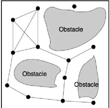
2.1.1.3 Cell and portal graphs

A Cell and Portal Graph (CPG) (TELLER, 1992) represents a method of abstracting the geometry of virtual environments. Generally, within indoor environments, the graph nodes (cells) indicate navigable regions such as rooms, whereas the portals represent entrance/exit points such as doors. For outdoor environments, cells can represent pedestrian pathways and portals are placed between pathways and crossings (LERNER et al., 2006; PELECHANO et al., 2008). After setting up the environment, the problem of navigating in a CPG is reduced to getting from a cell to another through a sequence of cells and portals (PETTRÉ et al., 2005; PELECHANO; BADLER, 2006; PELECHANO et al., 2008). Some examples of CPG can be seen in ﬁgures 6 and 7.

Figure 6 – An example of CPG. The portals are in green and the cells are represented by the colored polygons. A vertex is placed in each one of the cells and two cells are connected if they share a portal.

Source: Lerner et al. (2006).

2.1.1.4 Guidance fields

(33)

31

Figure 7 – Floor plan of a building and its corresponding CPG.

Source: Pelechano et al. (2008).

taking into account the repulsion caused by the obstacles and the attraction caused by the goal. Generally, in a potential ﬁeld method, the environment is discretized in a regular grid, where each cell has a potential value which corresponds to the attraction and repulsion forces acting on it. Once the gradient is computed based on the potential values of each cell, it is possible to follow it to reach low potential values, usually representing a goal. This method has the same problems regarding discretization as those found in discrete methods. Figure 8 shows a representation of a potential ﬁeld in an environment with a central obstacle.

Figure 8 – Potential ﬁeld representing an environment with a central obstacle.

Source: Warren (1989).

In (CHENNEY, 2004), the author proposed a similar approach where tiles with precomputed vector fields are used to compose the field of vectors representing large flows. In other words, through the production of tiles with different configurations it is possible to create scalable scenarios with varied flows. Figure 9 shows the tool used for composing scenarios with tiles.

(34)

32

Figure 9 – Tool used for composing scenarios with precomputed ﬁelds of vectors.

Source: Chenney (2004).

explicit collision avoidance. For this method, the grids’ discretization highly aﬀects the performance because the potential ﬁelds are dynamic and need to be computed for every simulation’s time-step. Figure 10 shows an overview of the algorithm proposed in (TREUILLE et al., 2006).

Figure 10 – Overview of the algorithm proposed for creating dynamic potential ﬁelds.

Source: Treuille et al. (2006).

2.1.1.5 Environment modeling

(35)

33

For that reason, techniques for automatic creation of topological representations have been developed. In (HAUMONT et al., 2003), the authors presented an algorithm for generating volumetric CPGs for indoor scenarios based on an adaptation of the 3-D watershed transform algorithm, computed on a distance-to-geometry sampled field. The environment is “flooded” from the local minima, and each minimum produces a region (room). Portals are created between regions when they get in contact during the flooding process (Figure 11). The algorithm classifies, automatically, each room as a cell and the openings (doors and windows) as portals, thus, being able to generate the CPG of any indoor environment.

Figure 11 – Flooding process used to generate the environment’s CPG.

Source: Haumont et al. (2003).

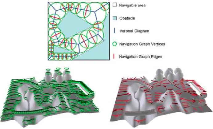
In (PETTRÉ et al., 2005), the authors proposed an approach based on a spatial structuring technique that automatically decomposes multilayered or uneven terrains into corridors giving rise to a navigation graph to be used for path planning. In this method, the space is divided into free spaces and obstacles to be avoided. At ﬁrst, it computes a Voronoi diagram of the free-space and, then, it builds a set of collision-free convex cells along the diagram. The navigation graph is obtained from the adjacency graph of the cells (Figure 12). The novelty of this work was to extend a basic navigation graph for terrains with multiple layers by classifying some areas with free spaces as obstacles based on the terrain’s slope.

(36)

34

Figure 12 – Navigation Graphs principles. Top: example of a Navigation Graph in a 2-D academic example. Bottom: Vertices (left) and Edges (right) of a Navigation Graph computed for a natural scene.

Source: Thalmann and Musse (2013).

Figure 13 – Example of partitioned scenario, where the buildings are in white and partition cells are in blue. On the left, a BSP (Binary Space Partitioning) partition and, on the right, a partition produced by the algorithm proposed by (LERNER et al., 2006)

Source: Lerner et al. (2006).

(37)

35

navigation. The topological map contains nodes which correspond to regions within the environment and edges representing accessibility between regions. The path maps include a quadtree map which supports global, long-range path planning and a grid map which supports short-range path planning.

Figure 14 – Hierarchical representation of a building.

Source: Shao and Terzopoulos (2007).

In (GERAERTS; OVERMARS, 2007), the authors presented the Corridor Map Method (CMM). That method, in an offline construction phase, creates a system of collision-free corridors for the static obstacles in an environment, and then, in the query phase, it plans paths inside the corridors for different types of characters that avoid dynamic obstacles. The authors use a method based on medial axis to represent free-space as a graph where the edges correspond to collision-free corridors. Each edge of the graph encodes a local path together with a maximum clearance radius which can be used to find paths with arbitrary clearance. Figure 15 shows a comparison of the CMM with two other methods.

Several methods aiming at reproducing free-space within environments by using meshes have been pro-posed. In (LAMARCHE; DONIKIAN, 2004), the authors used the Delaunay triangulation to compute a subdivision of convex cells of the free-space while maintaining the information about the local bottlenecks to represent the topological connectivity of 3-D environments. Other approaches explore the Voronoi diagram, as in (HOFF III et al., 1999) where a Voronoi representation of the static environment is precomputed for path planning; and in (SUD et al., 2007a) where the authors presented the Multi-agent Navigation Graph (MaNG) which is built dynamically using discrete Voronoi diagrams. The MaNG is used to compute simultaneously the maximum clearance paths for a set of agents which move with independent goals. In (KALLMANN, 2010), the author proposes a method for ﬁnding optimal paths with arbitrary clearance directly from a tri-angulation. The method proposed introduces a new local clearance property which facilitates the eﬃcient computation of the path clearance in a triangulated mesh.

(38)

36

Figure 15 – Three methods for path ﬁnding. (a) The A* algorithm ﬁnds the shortest path in the displayed grid, consisting of 1792 nodes and 3321 edges. (b) The PRM-graph is almost six times as small. (c) The CMM-graph is the smallest one containing 44 nodes and 50 edges.

Source: Geraerts and Overmars (2007).

dynamic obstacles and the interaction forces among the agents.

2.1.2 Local path planning

Local path planning can be deﬁned as:

The layer of intelligence that interfaces with navigation to move an agent along its planned path by performing a series of successive local searches, taking into consideration locomo-tion constraints such as turning capabilities and limits on movement velocity, as well as dynamic objects in the environment such as other agents (KAPADIA; BADLER, 2013).

(39)

37

The various existing solutions for this problem can be classified in several ways according to their common features. Some authors choose to classify them according to the way the agents are managed. In this case the approaches can be classified as: macroscopic or microscopic. Macroscopic approaches are concerned with the global crowd flow, regardless of the local interactions between agents, whereas microscopic approaches model local interactions between agents which influence each other’s motion. In the case of microscopic approaches, collective behaviors and global patterns emerge as a consequence of the agent’s local interactions. Other authors prefer to classify approaches according to their abilities of collision prediction. In this case, the different approaches are classified as predictive or reactive, depending on whether they allow anticipated reactions based on motion prediction or purely reactive motion. In (ZHENG et al., 2009), the authors present some features to classify approaches for crowd evacuation simulation. In this section, the algorithms were classified in the following categories based on the techniques used for collision avoidance: rule-based, particle-based, cellular automata, guidance fields, velocity-based, data-driven, based on synthetic vision and hybrid.

2.1.2.1 Rule-based models

In 1987, Reynolds presented a rule-based model, where the concept of boids (“bird-oid” contraction) was introduced. The author made these agents called boids behave as a flock through the combination of three simple individual rules, where the boids should: avoid collisions (separation), keep the same velocity (align-ment) and stay close to each other (cohesion). Rule-based models allow characterizing the agents individually with unique behaviors not only focusing on collision avoidance, making it possible to model heterogeneous agents with complex behaviors formed by the combination of simple behaviors. In 1999, Reynolds expanded his previous work by defining steering behaviors for autonomous agents (e.g., seek, flee, pursuit, evasion) (Figure 16).

Figure 16 – Examples of rules. Seek and ﬂee (left). Pursuit and evasion (right).

Source: Reynolds (1999).

(40)

38

2.1.2.2 Particle-based models

The interest in particle-based models arose given their ability to simulate crowd evacuation from buildings considering physical aspects. In (HELBING; MOLNÁR, 1995), the authors proposed a model where the agents move according to repulsive forces (exerted by other agents, objects, walls, etc.) and attractive forces (exerted by friends, objectives, etc.) trying to reach the position of their goals within the environment as comfortably as possible. This model naturally simulates agents’ self-organization in collective phenomena. Combining socio-psychological and physical forces, Helbing et al. (2000) proposed a particle-based model capable of simulating crowds in panic situations. The algorithm managed to reproduce many observed phenomena including: clogging effects at bottlenecks (Figure 17) and the corresponding increase of pressure, jamming at widenings, the “faster-is-slower” effect, inefficient use of alternative exits and initiation of panics by couterflows and impatience.

Figure 17 – Clogging eﬀect at a bottleneck reproduced with Helbing’s model.

Source: Helbing et al. (2000).

This type of model can be adapted to many situations just by adding new attractive and repulsive forces, according to the behavior expected for the crowd. In (COURTY; MUSSE, 2005), a repulsion force was added to Helbing’s model (HELBING et al., 2000) so as to make the crowd avoid places with smoke while trying to evacuate a building (Figure 18). In (BRAUN et al., 2003), the authors extended Helbing’s model to include individualism. Particle-based models have also been used for studying group behavior and their eﬀects on crowd dynamics (MOUSSAÏD et al., 2010; XU; DUH, 2010). Despite being particularly suitable for simulating emergency situations, this type of model can also be adapted for simulating common situations as can be seen in (PELECHANO et al., 2007).

A diﬀerent approach was proposed by (HEIGEAS et al., 2003). In this case, the agents’ interactions were modeled as a mass-spring-damper system, where stiﬀness and viscosity terms change with respect to the relative distance between the agents. Particle-based models are inherently reactive, i.e., agents do not anticipate their motion with respect to other agents in collision course, resulting in visually unpleasant artifacts in sparse environments. However, it is possible to minimize this drawback by adding an evasion force so as to make the agents react to future collisions in advance, as presented in (KARAMOUZAS et al., 2009).

2.1.2.3 Cellular automata models

(41)

39

Figure 18 – Crowd being repulsed by places with smoke while evacuating a building.

Source: Courty and Musse (2005).

simulated.

A cellular automaton evolves in discrete time steps, with the value of the variable at one cell being affected by the values of variables at the neighboring cells. The variables at each cell are updated simultaneously based on the values of the variables in their neighborhood at the previous time-step and according to a set of local rules (PELECHANO et al., 2008; WOLFRAM, 1983).

When used for simulating crowds, those rules are deﬁned to control the agents’ behaviors during the simula-tion.

Although fast and simple to implement, cellular automata models (DIJKSTRA et al., 2001; SCHAD-SCHNEIDER, 2001; TECCHIA et al., 2001; BURSTEDDE et al., 2001; KIRCHNER; SCHADSCHAD-SCHNEIDER, 2002; KIRCHNER et al., 2003) do not allow physical contact between agents, because each cell can be occu-pied by only one agent each time. This restriction causes this type of model to reproduce unrealistic results in high density situations (Figure 19), making them impracticable for some applications such as entertainment. Aiming at creating more realistic behavior in high density situations, in (LOSCOS et al., 2003), the authors adapted their model for collision avoidance to deal with several situations, enabling the cooperation between agents for decision-making, allowing the emergence of pedestrian ﬂow in the crowd.

Figure 19 – Room evacuation simulation using a cellular automata model. It is possible to notice the orga-nization of the agents in a regular grid.

(42)

40

2.1.2.4 Guidance field models

Models based on guidance fields can be used for both global (Section 2.1.1.4) and local path planning. As presented before, guidance fields can be manually defined by setting flow tiles to compose the field (CHENNEY, 2004). In (PATIL et al., 2011), the field is generated procedurally, but it can be influenced by user interaction (Figure 20 left) or by motion flow fields extracted from crowd video footage. Kapadia et al. (2009b) use egocentric fields to determine the optimal path that an agent can take at short-term (Figure 20 right). The main drawback of using local guidance fields is that they can easily lead agents to local minima. Figure 20 – Example of guidance fields. Field updated by user interaction (left) and egocentric field (right).

Source: Patil et al. (2011) (left) and Kapadia et al. (2009b) (right).

As it was briefly presented in Section 2.1.1.4, guidance fields can also be generated by using potential fields. In this case, each cell in the grid has a potential positive value which decreases according to the proximity of the goal. Goal cells must have a zero value so as to attract the agents, whereas obstacle cells must have high values to repulse them. This way, a gradient is formed indicating the path from each cell to the goal. Hughes (2002, 2003) presented a model where partial differential equations were defined to describe crowd dynamics. In this model, the agents are converted to a density field which is used to generate the potential field. Treuille et al. (2006) improved Hughes’s model to reach more realistic crowd behavior. Their model separates agents in groups with common goals, where these groups represent the environment as a grid of cells. Then, for each group, a potential field is computed. In (JIANG et al., 2010), the authors adapted Treuille’s model to deal with more complex environments. Models based on dynamic potential fields have as main advantage the possibility of simulating realistically the behavior of several agents in real-time. Nevertheless the process of generating potential fields is computationally expensive and, consequently, only a small number of groups (goals) is supported. Recently, Dutra et al. (2013) proposed a multipotential field method for allowing scalable behaviors in Treuille’s model (Figure 21).

2.1.2.5 Velocity-based models

(43)

41

Figure 21 – Example of multipotential ﬁelds. Eight potential ﬁelds are used to change momentarily the agents’ main goals.

Source: Dutra et al. (2013).

In the ﬁeld of robotics, there is the concept of Velocity Obstacle (VO), introduced by Fiorini and Shiller (1998), where a robot is capable of avoiding collisions with obstacles based on their velocities. The method consists of selecting a velocity in the velocity-space which allows the robot to avoid collisions with the static and moving obstacles based on their positions and velocities. This concept has been widely used by velocity-based models for simulating crowd behavior. In 2008, van den Berg et al. (2008a, 2008b) presented the concept of Reciprocal Velocity Obstacle (RVO) which extends the VO concept to guarantee safe and oscillation-free navigation among agents by considering the reactive behavior of the other agents, assuming that the agents avoid each other in the same way. Since then many contributions have been made to this approach. In (GUY et al., 2009), the authors presented a parallel algorithm which uses a discrete optimization method. The most recent evolution of velocity-based obstacles is represented by the Optimal Reciprocal Collision Avoidance (ORCA) approach (BERG et al., 2011), which eﬃciently computes the optimal solution (maximum collision free velocity closer to the comfort velocity) in the velocity-space, hence reciprocally avoiding collisions between agents in a near future (Figure 22).

This type of model can treat collisions among several agents and obstacles eﬃciently (thanks to its parallelizable nature) allowing to simulate crowds with visually pleasant trajectories in real-time; however this realism decreases when the crowd density increases. They can also expose artifacts when dealing with symmetric situations.

2.1.2.6 Data-driven models

(44)

42

Figure 22 – (a) A conﬁguration with eight agents. Their current velocities are shown using arrows. (b) The half-planes of permitted velocities for agent A induced by each of the other agents. The dashed region contains the velocities for A that are permitted with respect to all other agents. The arrow indicates the current velocity of A.

Source: Van den Berg et al. (2011).

and according to similar scenarios found in the database.

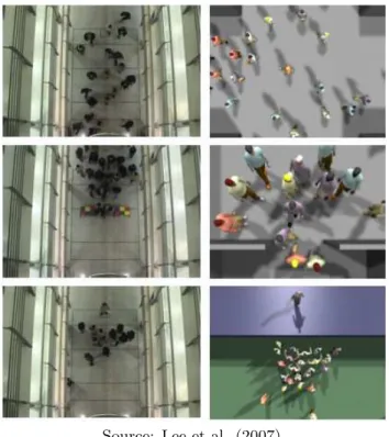
Pettré et al. (2009) presented a model able to simulate and reproduce experimental trajectories obtained from observations of real interactions between walkers. In (LERNER et al., 2009), the authors developed a method which, given a database of behaviors extracted from real crowd footage, is able to select from the database the behavior which is the most representative of the agent’s current situation. Paravisi et al. (2008) adapted Treuille’s model (TREUILLE et al., 2006) to reproduce crowd and group behavior extracted from video footage. The authors, in (JU et al., 2010), presented a method which combines diﬀerent data from several existing crowds to generate a new crowd animation. This data can be obtained from real crowds or virtual ones simulated by other models (Figure 24).

As stated initially, the input data need not necessarily be obtained through computer vision techniques as in (GUY et al., 2011), where the authors use perceptual studies to aﬀect the agents’ personalities, thus generating heterogeneous crowds. Recently, in (CHARALAMBOUS; CHRYSANTHOU, 2014), the authors introduced a structure called perception-action graph (PAG) for accelerating and improving the quality of data-driven crowds. The PAG handles the input examples as a graph, which is used at run-time to eﬃciently synthesize believable virtual crowds.

(45)

43

Figure 23 – Real data (left) and reproduced behavior (right).

Source: Lee et al. (2007).

Figure 24 – Real data (top) and reproduced behavior (bottom).

Source: Ju et al. (2010).

i.e., a behavior recorded in a speciﬁc situation may not work in a diﬀerent context.

2.1.2.7 Models based on synthetic vision

(46)

44

Agents would only interact if falling in such ﬁeld of view.

Figure 25 – Vision as a geometrical area. A vision of a ﬁsh (left) and a vision of a boid (right).

Source: Tu and Terzopoulos (1994) (left) and Silva et al. (2010) (right).

The first explicit simulation of locomotion using the agents’ vision was introduced in (RENAULT et al., 1990). In (NOSER et al., 1995), the authors used the agents’ vision to identify objects within an environment. Kuffner and Latombe (1999) used synthetic vision to allow agents to explore and to navigate within unknown environments. The authors in (PETERS; O’SULLIVAN, 2003) used synthetic vision to find interesting areas in the agent’s vision which could attract its attention and thus improve the feeling of presence within the virtual environment.

Ondřej et al. (2010) proposed a novel synthetic-vision approach for crowd simulation. Their model transforms the visual input of each agent into images containing information which allows detecting risk of collisions with any obstacle or agent in the scene (Figure 26). Agents react to the stimuli by turning to avoid a future collision when detected with anticipation and slowing down to avoid an imminent collision. Despite the good results reported, Ondřej’s model suﬀers from important drawbacks. This model and the model proposed by this thesis are strongly related, for this reason Section 2.2 is dedicated to present and to discuss the Ondřej’s model with more details.

Figure 26 – Representation of the agent’s visual perception.

Source: Ondřej et al. (2010).

(47)

45

the second rule is used to adapt speed according to the agent’s reaction time and the ﬁrst obstacle in the walking direction. Body collisions are avoided by using a particle-based algorithm. Despite resorting to the agent’s vision, it is not clear in the article whether this vision is a synthetic one or a geometrical representation. Recently, Rio et al. (2014) investigated the optical information used to control walking speed in pedestrian following. From the results of this investigation, the authors could derive a visual control law for one-dimensional following. This law is based on the optical expansion of the follower, where the follower accelerates if the leader’s visual angle is decreasing, decelerates if it is increasing, and maintains the current speed if visual angle is constant.

Models based on synthetic vision are very promising, allowing reproducing behaviors more closely to reality than those produced by traditional models, provided that the data obtained through the vision is interpreted properly. Those results come with a high computational cost, although, the rapid evolution of graphic cards suggests this approach will soon become more popular for real-time applications such as games.

2.1.2.8 Hybrid models

Each type of model has advantages and disadvantages. Thus, the idea of combining the best features of the existing models gave rise to the hybrid models. In (PELECHANO et al., 2007), the authors captured the best aspects of rule-based and particle-based models, and created a new model which used psychological, physiological and geometrical rules combined with physical forces to reproduce heterogeneous agents and to guide them within an environment. Yersin et al. (2008) proposed an architecture for simulating crowds which divides the environment in three regions of interest (ROI) according to the distance to the camera (the closer, the more important). Each ROI is ruled by a different technique of path planning. In regions of no interest, the planning is ruled by a navigation graph and collisions are not avoided; in regions of low interest, the planning is also ruled by a navigation graph and collisions are avoided resorting to the Reynolds’s concepts (1999); and finally, in high interest regions, both path planning and collision avoidance are ruled by potential fields, similar to (TREUILLE et al., 2006).

In (XIONG et al., 2010), the authors proposed an architecture where two models (a macroscopic and a microscopic) coexist in a simulation and work in a collaborative way, resorting to the benefits of each when necessary. The environment is divided in partitions and each of them is ruled by one of the models at a given instant. Narain et al. (2009) presented a model based on potential fields, but which solves local collisions using a geometrical model. First, the path of the agents is planned globally and their comfort velocities are set; then, locally, their velocities are adapted according to the density of the cell where the agents lie; after defining the velocities, the minimum distance among the agents is assured. In (SINGH et al., 2011), the authors described a framework that integrates multiple models which are used according to the agent’s current situation. Finally, the authors, in (GOLAS et al., 2014), proposed an approach which blends results from continuum and discrete algorithms, based on local density and velocity variance. Their hybrid method has seamless transitions between the continuum and discrete representations.

(48)

46

2.1.3 Path planning remarks

As it was stated at the beginning of this chapter, path planning is a research field widely explored, motivated by several problems found in the robotics field, entertaining industry and civil engineering, just to name a few. The works presented here are just some of the most relevant works that can be found in the literature. Most of the works can fit into more the one classification, for example, models based on synthetic vision can also be considered velocity-based approaches, since the agents take into account the movement of the obstacles to anticipate their motion. On the other hand, some models need specific classification given their very specific properties. Bicho et al. (2012), for example, proposed an algorithm for simulating crowds based on the modeling of leaf venation patterns and the branching architecture of trees. This model uses the concept of space colonization to model crowd behavior.

In some cases, animating crowds in huge and complex environments for long periods can be very chal-lenging and diﬃcult with the traditional crowd simulators. This need of handling dense populations in large-scale environments gave rise the models based on crowd patches. A crowd patch is a block containing precomputed local crowd simulation. Several patches can be designed with diﬀerent animations. Then, for animating a crowd, it is necessary just to connect patches in space and time (Figure 27). Crowd patches provide endless animation in real-time, nevertheless interactivity is not allowed since the agents cannot adapt their precomputed paths (LEE et al., 2006; YERSIN et al., 2009; JORDAO et al., 2014).

Figure 27 – Crowd patches used for crowd simulation.

Source: Yersin et al. (2009).

(49)

47

2.1.4 Social behavior

Several techniques have been proposed over the years focusing on navigation and collision avoidance in crowds represented as conglomerations of agents with global goals. However, in real crowds there are several social interactions, since people interact with the environment and with each other. While most of the crowd behavior studies consider only interactions among isolated individuals, a recent study demonstrated that up to70% of the pedestrians observed in crowds walk in groups (MOUSSAÏD et al., 2010). In this case, groups

in the sociological sense, i.e., not only referring to the proximity of individuals, but the individuals with social relationships intentionally walking together, such as friends or members of the same family.

Reynolds (1987) in his pioneering work simulated a flock of boids, which is a group formation, using a set of rules (alignment, cohesion and separation). Musse and Thalmann (1997) used sociological concepts to describe a rule-based model for simulating the relationship of groups in a crowd. An agent interacts with a group according to its emotional status, the level of relationship with the group, and its level of dominance. With these characteristics and the rules established by the model, the authors could simulate some sociological effects in crowds, such as grouping, polarization and adding. In 1999, Reynolds introduced more rules for steering agents and, through the combination of some of them, he described the leader following behavior (Figure 28). In (QIU; HU, 2010), the authors simulated intra-group and inter-group relationships in a model based on (REYNOLDS, 1999). In this model, two-dimensional matrices were used to establish the relationships among the agents in the same group and the relationships among groups. Recently, Lemercier and Auberlet (2015) presented behavioral rules based on perception in which agents analyze the situation to adopt different behaviors accordingly (following and group collision avoidance behavior).

Figure 28 – Leader following behavior.

Source: Reynolds (1987).

In (BRAUN et al., 2003), the authors added an altruism force to the particle-based model proposed by Helbing et al. (2000). This force is used to keep the agents belonging to the same family together. The experiments performed with this model showed that the addition of the altruism force made altruist agents tend to rescue dependent agents (Figure 29). Xu et al. (2010) developed a particle-based model to simulate groups of two agents. Then, they studied the impact of these bonding eﬀects on crowd behavior.

(50)

48

Figure 29 – Altruism force being used to keep groups together.

Source: Braun et al. (2003).

tend to walk side by side, forming a line perpendicular to the motion direction; whereas, in high density, the members tend to form a V-like pattern (Figure 30). The authors demonstrated, by adding a group force to a particle-based model, that the V-like pattern facilitates social interactions within the group, but reduces the ﬂow because of its “non-aerodynamic” shape. The authors conclude that: “crowd dynamics is not only determined by physical constraints induced by other pedestrians and the environment, but also signiﬁcantly by communicative, social interactions among individuals”.

Figure 30 – Average patterns of organization of groups with two to four individuals.