AbstrAct Aegialomys xanthaeolus (Cricetidae: Sigmodontinae) inhabits the arid montane areas of

O

S

V

CHARACTERSOF

A

(T

, 1894)

(C

: S

)

E

P

J

R. P

A

R. P

ABSTRACT

Aegialomys xanthaeolus (Cricetidae: Sigmodontinae) inhabits the arid montane areas of western Ecuador and Peru, and higher elevations in the upper Marañón valley in northern Peru. Some researchers have included this species in broader systematic assessments over the years, but there are no comprehensive studies focusing on intraspecific variation. There are sev-eral sources of intraspecific phenotypic variation, including sexual dimorphism and age. These sources may confound the assessment of similarity/dissimilarity among populations, therefore it is essential that non-geographic variation is evaluated before studies on geographical variation and species delimitation are carried out. Here we summarize existing information regarding the geographical distribution of A. xanthaeolus and evaluate variation related to sex and age. We analyzed 19 traditional cranio-dental measurements taken from specimens housed in sci-entific collections, and organized the collecting localities of specimens examined in a gazetteer and plotted them on a distribution map. Uni and multivariate statistical analyses allow us to assert that age variation was significant, as age classes 3, 4 and 5 can be pooled for the subse-quent analysis of geographic variation and that sexual dimorphism is not a consistent compo-nent of variation within this species in the conticompo-nental samples, when considering samples from the same locality, or localities close to each other.

Keywords: Geographic Distribution; Skull; Ontogeny; Sexual Dimorphism; Morphometrics.

INTRODUCTION

The cricetid rodents of the genus Aegialomys are a trans-Andean group, distributed throughout the open habitats of the western Peruvian and Ecuador-ean Andes, including the Galapagos Island (Musser & Carleton, 2005). The most recent contribution

(Weksler et al., 2006) that studied the xanthaeolus

species group of the former genus “Oryzomys” (sensu lato, see Musser et al., 1998; Percequillo, 1998, 2003; Weksler, 2003; Musser & Carleton, 2005), proposed a new generic name, Aegialomys, and recognized two species: Aegialomys galapagoensis (Waterhouse, 1839) and Aegialomys xanthaeolus (Thomas, 1894).

1. Departamento de Ciências Biológicas, Escola Superior de Agricultura “Luiz de Queiroz”, Universidade de São Paulo, Avenida Pádua Dias, 11, Caixa Postal 9, 13418-900, Piracicaba, São Paulo, Brasil.

According to Weksler et al. (2006) Aegialomys xanthaeolus inhabit the dry montane areas at western regions of Ecuador and Peru, reaching the high eleva-tions (about 2500 m) in the upper Marañon valley, northern Peru. These authors describe A. xanthaeolus

as a medium size rodent, with very long and dense dorsal pelage, coarsely grizzled yellowish- or grayish-brown and ventral pelage paler, with ventral hairs al-ways gray-based; with small pinnae and mystacial vi-brissae not extending posteriorly beyond pinnae when laid back; with hind foot with conspicuous tufts of ungual hairs; with tail distinctly longer than head and body, weakly to distinctly bicolored. This species also exhibit small to moderately large skull, with strongly beaded supraorbital ridges, long incisive foramina, usually long palate, large sphenopalatine vacuities, the derived pattern of carotid circulation (type 3 of Voss, 1988), and large auditory bullae.

Over the years, few publications dealt with some biological aspects (karyology, morphological com-parisons, phylogenetic position) of oryzomyine taxa, including Aegialomys xanthaeolus (Thomas, 1894; Heller, 1904; Cabrera, 1961; Gardner & Patton, 1976; Patton & Hafner, 1983; Weksler, 2003, 2006; Weksler et al., 2006), but none of them studied the intra-specific variation structure, aiming to evaluate the validity of some species group taxa associated with this species (Weksler et al., 2006).

According to Reis et al. (1990), description of patterns of variation in morphologic and genetic char-acters within and among populations is essential to detect independent evolutionary subunits, an impor-tant aspect to comprehend species variation and lim-its. Mayr (1969) stated that there are several sources of phenotypic variation among species, which he classi-fied as non-genetic (ontogenetic, seasonal, social, eco-logic and traumatic variation) and genetic (related to sex, continuous and discontinuous variation). These variations can obscure the evaluation and recognition of similarity and dissimilarity among populations (Ab-del-Rahman et al., 2008). It is therefore fundamental that non-geographic variation, such as sexual dimor-phism and ontogenetic variation should be clarified before studies related to geographic variation and spe-cies delimitation are carried out (Thorpe, 1976; Patton & Rogers, 1983; Reis et al., 1990, 2002). In studies fo-cusing on rodents, sample sizes are frequently too small to enable the assessment of all these genetic and non-genetic variation. Therefore, the majority of non-geo-graphic analyses only examine sexual dimorphism and ontogenetic variation (Abdel-Rahman et al., 2008).

Although usually neglected in recent times, study of non-geographic variation attracts the interest

of biologists since Darwin (Abdel-Rahman et al.,

2008). There are several examples that documented shape differences among individuals of one popula-tion or between co-specific populapopula-tions, than among closely related species (Mayr, 1977). Among mam-mals, taxa that have noticeable difference in body size regarding sex belong to the orders Primates and Proboscidea, to the suborders Odontoceti, Pinnipe-dia, Ruminantia and to families Macropodidae and Mustelidae (Weckerly, 1998).

In the present contribution, we evaluate and describe non-geographic variation in Aegialomys xan-thaeolus, especially related to sexual and age variation; and present information on the geographical distribu-tion of this species.

MATERIAL AND METHODS

Samples

We examined specimens from the following museum collections: American Museum of Natural History, New York, United States (AMNH); Natural History Museum, London, England (BMNH); The Field Museum, Chicago, United States (FMNH); Louisiana State University, Museum of Zoology, Ba-ton Rouge, United States (LSUMZ); Museum of Ver-tebrate Zoology, University of California, Berkeley, United States (MVZ); Smithsonian Institution Na-tional Museum of Natural History, Smithsonian In-stitution, Washington D.C., United States (NMNH).

Gazetteer

The collecting localities are organized in alpha-betical order by country, state or province and locality. Descriptions of localities, geographical coordinates and elevation data were obtained as accurately as possible from specimen labels. The following sourc-es were also used to obtain geographic coordinatsourc-es: United States Board on Geographical Names (US-BGN, NIMA; see http://gnswww.nga.mil/geonames/ GNS/index.jsp), Stephens & Traylor (1983), and Paynter (1993).

Definition of Locality Clusters

localities, and thus making more feasible analyses of non-geographic variance. We defined some criteria to pool these localities, in order to avoid the pooling of samples that could be subjected to geographic varia-tion. We only clustered samples: from the same alti-tudinal gradient; that are not separated by large rivers or other geographic accident, such as cliffs, ravines, high mountains (e.g., Andean Cordillera); and, that are surrounding a larger sample, within a radius of

ca. 50 km.

On the other hand, in order to compare the non-geographic variation on the whole distribution of genus (except Galapagos Islands samples) with the non-geographic variation observed in the small clus-ters of localities, we also pooled all available samples in one large Aegialomys sample.

Cranio-Dental Measurements

We obtained measurements (in mm) from the skull and the teeth of all specimens examined. A 0.01 mm precision caliper was used to obtain the mea-surements of the following cranio-dental dimensions:

Total length of skull (TL): measured from the anterior margin of nasals to the posteriormost portion of the occipital;

Condylo-incisive length (CIL): measured from the greater curvature of the upper incisor to the articular surface of the occipital condyle, on the same side of the skull;

Length of diastema (LD): measured from the crown of the first upper molar to the inner side of the base of the upper incisor on the same side of the skull;

Length of molars (LM): measured from the anterior surface of the first upper molar to the posterior surface of the third upper molar, at the crown of the molars;

Breadth of M1 (BM1): greatest breadth of the first up-per molar measure of the base crown, the height of the protocone;

Length of incisive foramen (LIF): the greatest length measured from the anterior edge to posterior edge of incisive foramen;

Breadth of incisive foramen (BIF): the greatest internal breadth, measured on the lateral margins of the inci-sive foramen;

Palatal breadth (PB): measured in the external later-al portion of the maxillary, between the second and third molar;

Breadth of interparietal (BIP): greatest breadth of in-terparietal bone;

Length of interparietal (LIP): greatest length (antero-posterior) of interparietal bone;

Breadth of rostrum 2 (BR2): measured across the ros-trum, at the posterior extremity of the upper edge of the infraorbital foramen;

Length of nasal (LN): measured from the anteriormost end of the nasal to the naso-frontal suture;

Length of palatal bridge (LPB): measured from the posterior margin of incisive foramen to the anterior margin of mesopterygoid fossa;

Least interorbital breadth (LIB): shortest distance through the frontals in the orbital fossa;

Zygomatic breadth (ZB): greatest external distance of the zygomatic arches, close to the squamosal roots, measured across the skull;

Breadth of zygomatic plate (BZP): the shortest distance between the anterior and posterior margin of the infe-rior zygomatic root or zygomatic plate;

Condylo-zygomatic length (CZL): shortest distance between the posteriormost point of occipital condyle and the posteriormost point of the upper edge of the zygomatic notch;

Orbital fossa length (OFL): greatest dimension of the orbital fossa between the squamosal and maxillary roots of zygomatic arch;

Bullar breadth (BB): measured from the petrosal suture with the basioccipital to dorsal process of ectotympanic.

Sexual Dimorphism and Age Classes

Age class 1: First and second molars without apparent wear, with labial flexus open and conspicuous. Third molar is usually non-erupted or newly erupted, with the main cusps still closed, without dentine exposi-tion. Dorsal pelage is predominantly gray and ventral pelage is grayish.

Age class 2: In this class, first and second molars with minor wear, with main cusps high and with small exposure of dentine; some flexi closed, forming fos-sets (especially anteroflexus and posteroflexus). Third molar already showing wear, but minimal to moder-ate. Dorsal pelage is predominantly gray and ventral pelage is grayish.

Age class 3: First and second molar in this class with medium wear, with the cusps conspicuously eroded and with large dentin exposure; nearly all labial flexi closed (especially para-, meso-, and metaflexus) and some fossetes (posterofessete). Third molar exhibit marked wear, with nearly flat to flat surface. Dor-sal pelage is coarsely grizzled yellowish- or grayish-brown, with the aristiform hairs with the tip yellow and ventral pelage is pale yellow.

Age class 4: First and second molar with heavy wear, with flat and indistinct cusps and massive exposure of dentine; most fossetes eroded (para- and metafossete more persistent). Third molar appears quite flat, with major exposure of dentine. Dorsal pelage is coarsely grizzled yellowish- or grayish-brown, with the aristi-form hairs with the tip yellow and ventral pelage is cream.

Age class 5: Three molars are completely worn, with large exposition of dentine. Dorsal pelage is coarsely grizzled yellowish- or grayish-brown, with the aristi-form hairs with the tip yellow and ventral pelage is cream.

Statistical Analysis

The sample was first assessed for univariate nor-mality, according to the Kolmogorov-Smirnov test (KS) and for multivariate normality, according the Mardia Kurtosis test (Sokal & Rohlf, 1997; Kankain-en, et al. 2003).

We calculated descriptive statistics for samples and applied the t test to check for sexual dimorphism. We then employed analysis of variance (ANOVA and MANOVA) and Tukey’s post hoc test to check for age variation. Firstly, in the Aegialomys sample we

implemented the following analyses: age variation with males and females pooled, then age variation with sexes separated; sex variation, comparing males and females from age class 3 and class 4, separately. Secondly, we performed the same analyses in the se-lected largest available clusters of localities. This was conducted to evaluate different approaches to access non-geographic variation.

Principal Component Analysis and Discriminant Function Analysis were computed using a combina-tion of cranio-dental measurements. Principal Com-ponents were extracted from the correlation matrix and canonical variables were extracted for the Discrim-inant Function Analysis (Johnson & Wichern, 1999; Manly, 2005). These multivariate analyses were per-formed with the Aegialomys sample, since as an a priori

evaluation, PCA will summarize the entire variation of the sample, whether non-geographic or geographic.

RESULTS

Geographical Distribution

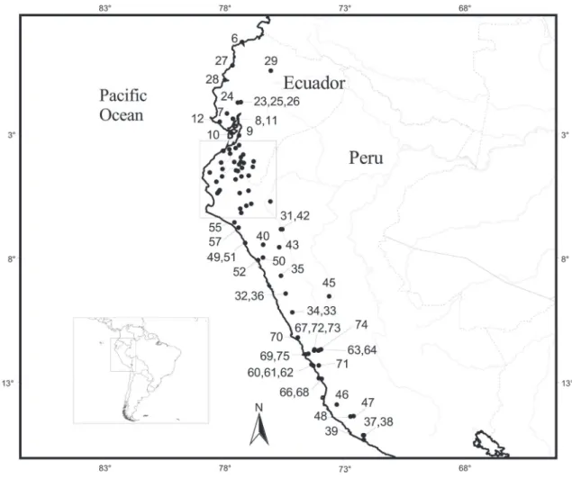
We examined 465 specimens (Appendix A), and based on the information provided by these we elabo-rated a gazetteer with 90 localities from Peru and Ec-uador (Appendix B) and an updated distribution map for the species (Fig. 1 and 2).

The distribution of Aegialomys xanthaeolus is limited by Esmeraldas (Esmeraldas Province, Ec-uador) to the north; by Chavina (Arequipa Depart-ment, Peru) to the south; by Hacienda Buena Vista, Chinchao (Huanuco Department, Peru) to the east; and the coastline of Ecuador and Peru to the west, except from its presence in a continental island, Isla Puna, in Ecuador. Altitudinal records of A. xanthaeo-lus range from sea level, in the localities Esmeraldas, Cuaque and Bahia de Caraquez (all located in Ecua-dor), to 2743 m in the locality 5 miles East of Yanyos (Peru).

This is a trans-Andean species, with most locali-ties (ca. 66%) located on the coastal lowlands of Peru and Ecuador and part of collection samples (ca. 34%) located in the Andean Cordillera, on the upper part of mountain slopes and on the deep portions of river valleys.

Definition of Locality Clusters

numbers of localities in the Table 1 corresponds to the number shown in the gazetteer given in Appendix B.

Intraspecific variation: Age and Sex

The univariate normality test Kolmogorov-Smirnov was applied to each of the nine geographic groups, and all variables showed a normal distribution (results not shown). Accordingly to Manly (2005), if all the individual variables under study are normally distributed, then it is plausible to assume that the mul-tivariate distribution is also normal. Nevertheless, we also performed Mardia Kurtosis test (p = 0,000) and its coefficient was 618.02, showing that all variables are also normally distributed in multivariate space.

Aiming to evaluate sex and age variation we perform a MANOVA with all specimens (Aegialomys

sample) and in the Isla Puna, respectively. The results of

first MANOVA for sex*ages effects are depicted in Ta-ble 2. Both age and sex, as well the interactions between factors were shown to be statistically different. The re-sults of the MANOVA for Isla Puna sample for sex*ages effects revealed (Table 3) that age, sex and interaction between these factors was not statistically different.

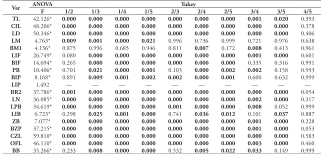
These discrepant results lead us to investigate the variation of univariate level, and we first conduct-ed a series of ANOVA’s and Student’s t analyses to test age and sex variation. Regarding age, we first com-pared the five age classes on the Aegialomys sample. The results (Table 4) showed that all variables, except LIP, showed differences among age classes. The post hoc Tukey test revealed significant difference between classes 1 and 2 for 12 variables, TL, CIL, LD, LM, LIP, BR2, LN, LPB, ZB, BZP, CZL and OFL; even when compared to other age classes, the class 1 is very different. Classes 2 and 3 differ in 12 variables TL, CIL, LD, LIF, BIF, BR2, BIP, LN, LPB, ZB, BZP,

CZL and OFL. Classes 3 and 4 were different on 14 variables, TL, CIL, LD, BM1, LIF, PB, BR2, LN, LPB, ZB, BZP, CZL, OFL and BB. The classes 4 and 5 did not show significant differences.

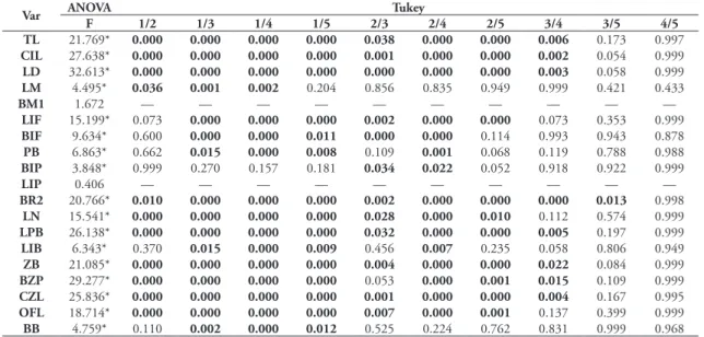
In addition we performed an ANOVA for the age classes within each sex separately. First within males, the results (Table 5) showed that all variables, except BM1 and LIP, showed differences among age classes. The post hoc Tukey test revealed significant dif-ference between classes 1 and 2 for 11 variables, TL, CIL, LD, LM, BR2, LN, LPB, ZB, BZP, CZL and OFL. Classes 2 and 3 are different for 12 variables TL, CIL, LD, LIF, BIF, BIP, BR2, LN, LPB, ZB, CZL and OFL. Classes 3 and 4 were different on 8 variables,

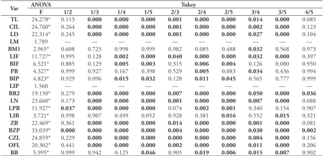
TL, CIL, LD, BR2, LPB, ZB, BZP and CZL. The classes 4 and 5 did not show significant differences again. Second within females, the results (Table 6) showed that all variables showed differences among age classes, except LM and LIP. The post hoc Tukey test revealed significant difference between classes 1 and 2 for LPB and BZP. Classes 2 and 3 differ in 10 variables, TL, CIL, LD, LIF, BR2, LN, ZB, BZP, CZL and OFL. Classes 3 and 4 were different for 13 variables, TL, CIL, LD, BM1, LIF, PB, LIP, LN, ZB, BZP, CZL, OFL and BB. The classes 4 and 5 did not show significant differences.

Subsequently we evaluated the age variation within the best sample, Isla Puna, but this group did

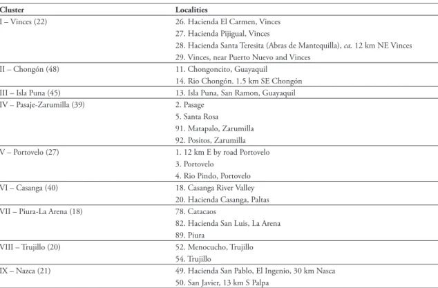
TABLE 1: Composition of Clusters (The numbers preceding the names of localities correspond to the index localities and the number beside the name of the group correspond to the total number of the individuals of the cluster).

Cluster Localities

I – Vinces (22) 26. Hacienda El Carmen, Vinces 27. Hacienda Pijigual, Vinces

28. Hacienda Santa Teresita (Abras de Mantequilla), ca. 12 km NE Vinces 29. Vinces, near Puerto Nuevo and Vinces

II – Chongón (48) 11. Chongoncito, Guayaquil 14. Rio Chongón. 1.5 km SE Chongón III – Isla Puna (45) 13. Isla Puna, San Ramon, Guayaquil IV – Pasaje-Zarumilla (39) 2. Pasage

5. Santa Rosa

91. Matapalo, Zarumilla 92. Positos, Zarumilla V – Portovelo (27) 1. 12 km E by road Portovelo

3. Portovelo

4. Rio Pindo, Portovelo VI – Casanga (40) 18. Casanga River Valley

20. Hacienda Casanga, Paltas VII – Piura-La Arena (18) 78. Catacaos

82. Hacienda San Luis, La Arena 89. Piura

VIII – Trujillo (20) 52. Menocucho, Trujillo 54. Trujillo

IX – Nazca (21) 49. Hacienda San Pablo, El Ingenio, 30 km Nasca 50. San Javier, 13 km S Palpa

TABLE 2: Results for the multivariate analysis of variance per-formed for the fixed effects of a priori ages, sex, and the interaction between them for total sample, on Aegialomys xanthaeolus specimens.

Hotelling’s Trace F

Hypothesis

df Error df Sig.

Age 1.347 3.744 84 934 0.000

Sex 0.150 1.679 21 235 0.035

Age*Sex 0.500 1.390 84 934 0.014 Values significant at the α = 0.05 level.

TABLE 3: Results for the multivariate analysis of variance per-formed for the fixed effects of a priori ages, sex, and the interaction between them for Isla Puna, on Aegialomys xanthaeolus specimens.

Hotelling’s Trace

F Hypothesis df

Error df Sig.

Age 16.346 0.000 36 0 0.890

Sex 34.277 1.904 18 1 0.971

FIGURE 2: Detail of map showing known collection localities for Aegialomys xanthaeolus.

TABLE 4: ANOVA followed by Tukey test between age classes for the entire sample of 19 cranio-dental variables. Values in bold represent statistical difference at 5% in Tukey test and the * represent statistical difference at 5% in ANOVA.

Var ANOVA Tukey

F 1/2 1/3 1/4 1/5 2/3 2/4 2/5 3/4 3/5 4/5

TL 42.126* 0.000 0.000 0.000 0.000 0.000 0.000 0.000 0.001 0.020 0.393

CIL 48.206* 0.000 0.000 0.000 0.000 0.000 0.000 0.000 0.000 0.000 0.378

LD 50.346* 0.000 0.000 0.000 0.000 0.000 0.000 0.000 0.000 0.000 0.406

LM 4.763* 0.009 0.001 0.000 0.021 0.996 0.736 0.999 0.721 0.976 0.638

BM1 4.136* 0.875 0.996 0.685 0.946 0.811 0.007 0.172 0.008 0.413 0.961

LIF 26.749* 0.080 0.000 0.000 0.000 0.000 0.000 0.000 0.001 0.000 0.601

BIF 14.694* 0.265 0.000 0.000 0.000 0.000 0.000 0.000 0.335 0.316 0.991

PB 10.406* 0.701 0.021 0.000 0.001 0.103 0.000 0.002 0.002 0.158 0.993

BIP 8.168* 0.891 0.009 0.001 0.002 0.002 0.000 0.001 0.600 0.632 0.999

LIP 1.492 — — — — — — — — — —

BR2 37.786* 0.001 0.000 0.000 0.000 0.000 0.000 0.000 0.000 0.000 0.054

LN 36.085* 0.000 0.000 0.000 0.000 0.000 0.000 0.000 0.002 0.000 0.317

LPB 34.619* 0.000 0.000 0.000 0.000 0.001 0.000 0.000 0.008 0.052 0.999

LIB 6.723* 0.298 0.025 0.001 0.000 0.741 0.036 0.012 0.101 0.037 0.887

ZB 7.077* 0.000 0.000 0.000 0.000 0.000 0.000 0.000 0.001 0.000 0.228

BZP 37.215* 0.000 0.000 0.000 0.000 0.000 0.000 0.000 0.001 0.000 0.053

CZL 59.810* 0.000 0.000 0.000 0.000 0.000 0.000 0.000 0.000 0.000 0.583

OFL 46.110* 0.000 0.000 0.000 0.000 0.000 0.000 0.000 0.003 0.000 0.460

FIGURE 3: Clusters tested in this study.

TABLE 5: ANOVA followed by Tukey test between age classes for the entire sample of 19 cranio-dental variables in males. Values in bold represent statistical difference at 5% in Tukey test and the * represent statistical difference at 5% in ANOVA.

Var ANOVA Tukey

F 1/2 1/3 1/4 1/5 2/3 2/4 2/5 3/4 3/5 4/5

TL 21.769* 0.000 0.000 0.000 0.000 0.038 0.000 0.000 0.006 0.173 0.997

CIL 27.638* 0.000 0.000 0.000 0.000 0.001 0.000 0.000 0.002 0.054 0.999

LD 32.613* 0.000 0.000 0.000 0.000 0.000 0.000 0.000 0.003 0.058 0.999

LM 4.495* 0.036 0.001 0.002 0.204 0.856 0.835 0.949 0.999 0.421 0.433

BM1 1.672 — — — — — — — — — —

LIF 15.199* 0.073 0.000 0.000 0.000 0.002 0.000 0.000 0.073 0.353 0.999

BIF 9.634* 0.600 0.000 0.000 0.011 0.000 0.000 0.114 0.993 0.943 0.878

PB 6.863* 0.662 0.015 0.000 0.008 0.109 0.001 0.068 0.119 0.788 0.988

BIP 3.848* 0.999 0.270 0.157 0.181 0.034 0.022 0.052 0.918 0.922 0.999

LIP 0.406 — — — — — — — — — —

BR2 20.766* 0.010 0.000 0.000 0.000 0.002 0.000 0.000 0.000 0.013 0.998

LN 15.541* 0.000 0.000 0.000 0.000 0.028 0.000 0.010 0.112 0.574 0.999

LPB 26.138* 0.000 0.000 0.000 0.000 0.032 0.000 0.000 0.005 0.197 0.999

LIB 6.343* 0.370 0.015 0.000 0.009 0.456 0.007 0.235 0.058 0.806 0.949

ZB 21.085* 0.000 0.000 0.000 0.000 0.004 0.000 0.000 0.022 0.084 0.999

BZP 29.277* 0.000 0.000 0.000 0.000 0.053 0.000 0.001 0.015 0.109 0.999

CZL 25.836* 0.000 0.000 0.000 0.000 0.001 0.000 0.000 0.004 0.167 0.995

OFL 18.714* 0.000 0.000 0.000 0.000 0.007 0.000 0.001 0.137 0.399 0.999

not address all age classes, this way the analysis of age variation (ANOVA) were conducted only in the classes 3, 4 and 5 (Table 7) showing that for variables TL, CIL, LD, BR2, LN, LPB, ZB, BZP and CZL there are significant differences between these three age classes. The post hoc Tukey test showed that for 8 variables, TL, CIL, LD, BR2, LPB, ZB, BZP and CZL the age 3 is significantly different from the age 4; for CIL, ZB and BZP, age 3 is significantly different from age 5, and for any variable the class 4 is signifi-cantly different from class 5.

Regarding sexual dimorphism in Aegialomys xanthaeolus, we also compared males and females on

Aegialomys sample with all age classes separately and then in the Isla Puna sample within classes 3 and 4 separately (we could not perform the analysis in class 5 due to small sample sizes), to avoid the influence of age variation in the samples. The results of the analy-sis in the Aegialomys sample are (see Table 8): in the class 1, only PB and BB showed significant difference between sexes; considering class 2, only TL and LN showed significant difference between sexes; regarding class 3, 13 variables showed significant difference: TL, CIL, LD, BIF, BR2, LN, LPB, LIB, ZB, BZP, CZL, OFL and BB; in class 4, only six variables showed sig-nificant difference, TL, CIL, LD, LIB, BR2 and CZL; and finally, specimens classified as class 5 exhibited no significant difference between sexes. On Isla Puna sample (Table 9), 13 variables showed significant dif-ference between sexes, TL, CIL, LD, LM, BIF, PB, LPB, LIB, ZB, BZP, BR2, CZL and OFL, for age

class 3. When considering class 4, only three variables (TL, CIL and LD), showed significant difference be-tween sexes.

To verify how sexual dimorphism is structured along the geography, comparisons were performed

TABLE 6: ANOVA followed by Tukey test between age classes for the entire sample of 19 cranio-dental variables in females. Values in bold represent statistical difference at 5% in Tukey test and the * represent statistical difference at 5% in ANOVA.

Var ANOVA Tukey

F 1/2 1/3 1/4 1/5 2/3 2/4 2/5 3/4 3/5 4/5

TL 24.278* 0.113 0.000 0.000 0.000 0.001 0.000 0.000 0.014 0.000 0.085

CIL 24.760* 0.264 0.000 0.000 0.000 0.001 0.000 0.000 0.002 0.000 0.123

LD 22.314* 0.245 0.000 0.000 0.000 0.001 0.000 0.000 0.027 0.000 0.104

LM 1.789 — — — — — — — — — —

BM1 2.965* 0.608 0.723 0.998 0.999 0.982 0.085 0.488 0.032 0.568 0.973

LIF 11.727* 0.995 0.128 0.002 0.000 0.040 0.000 0.000 0.032 0.000 0.397

BIF 6.521* 0.885 0.129 0.005 0.003 0.315 0.006 0.004 0.126 0.080 0.950

PB 4.327* 0.999 0.927 0.167 0.398 0.529 0.005 0.083 0.034 0.436 0.994

BIP 4.823* 0.929 0.096 0.015 0.032 0.128 0.011 0.045 0.565 0.777 0.999

LIP 1.560 — — — — — — — — — —

BR2 19.150* 0.279 0.000 0.000 0.000 0.007 0.000 0.000 0.050 0.000 0.036 LN 23.660* 0.173 0.000 0.000 0.000 0.001 0.000 0.000 0.007 0.000 0.088

LPB 11.927* 0.037 0.000 0.000 0.000 0.074 0.002 0.001 0.340 0.154 0.907

LIB 3.721* 0.998 0.907 0.499 0.052 0.928 0.381 0.016 0.552 0.015 0.321

ZB 22.469* 0.361 0.000 0.000 0.000 0.014 0.000 0.000 0.001 0.000 0.081

BZP 33.039* 0.000 0.000 0.000 0.000 0.004 0.000 0.000 0.030 0.000 0.002 CZL 24.859* 0.229 0.000 0.000 0.000 0.000 0.000 0.000 0.004 0.000 0.156

OFL 20.302* 0.441 0.000 0.000 0.000 0.002 0.000 0.000 0.011 0.000 0.206

BB 5.995* 0.999 0.942 0.125 0.046 0.905 0.019 0.006 0.015 0.007 0.902

TABLE 7: ANOVA followed by Tukey test between age classes 3, 4 and 5 for the cluster Isla Puna of 19 cranio-dental variables. Values in bold represent statistical difference at 5% in Tukey test and the * represent statistical difference at 5% in ANOVA.

Variable ANOVA Tukey

F 3/4 3/5 4/5

TL 3.797* 0.044 0.185 0.919

CIL 6.841* 0.007 0.029 0.794

LD 4.927* 0.016 0.119 0.944

LM 0.166 — — —

BM1 0.896 — — —

LIF 0.203 — — —

BIF 1.510 — — —

PB 0.014 — — —

BIP 1.097 — — —

LIP 0.278 — — —

BR2 4.943* 0.030 0.055 0.699

LN 3.389* 0.069 0.158 0.877

LPB 4.404* 0.034 0.097 0.818

LIB 0.676 — — —

ZB 11.917* 0.003 0.000 0.145

BZP 5.956* 0.040 0.013 0.305

CZL 5.855* 0.009 0.077 0.938

OFL 1.262 — — —

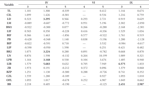
between male and female individuals with age classes separately for the clusters Pasaje-Zarumilla (IV), Ca-sanga (VI) and Nazca (IX; see Table 10); the small sample size of the other clusters precluded us to

conduct these comparative analyses. According to the availability of sample, differents age classes were tested in differents clusters. In the Pasage-Zarumilla (IV) sample, only class 3, 4 and 5 could be tested, the

TABLE 9: Results of Student t tests between sexes for the Isla Puna in age class 3 and 4 on 19 cranio-dental variables, containing the value of t. Values in bold represent statistical difference at 5%.

Variable 3 4

TL 2.745 2.194

CIL 2.923 2.146

LD 2.992 2.612

LM 1.222 -0.557

BM1 0.357 -0.586

LIF 1.760 1.017

BIF 2.726 0.423

PB 0.366 -0.023

BIP 1.343 0.432

LIP 1.601 1.379

BR2 3.015 3.001

LN 2.797 1.339

LPB 2.210 2.926

LIB 3.824 3.379

ZB 2.689 1.336

BZP 2.155 1.640

CZL 2.900 2.090

OFL 3.167 1.521

BB 2.576 -0.030

TABLE 8: Results of Student t tests between sexes for the total sample in each age class on 19 cranio-dental variables, containing the value of t. Values in bold represent statistical difference at 5%.

Variable 1 2 3 4 5

TL -0.988 2.691 2.745 2.194 -0.711

CIL -1.677 1.470 2.923 2.146 -0.431

LD -1.936 1.887 2.992 2.612 0.133

LM -0.850 -0.381 1.222 -0.557 -1.656

BM1 -1.286 -0.642 0.357 -0.586 -1.046

LIF -1.883 0.306 1.760 1.017 -0.599

BIF -0.855 -0.708 2.726 0.423 -1.156

PB -2.478 -0.575 0.366 -0.023 -0.079

BIP 0.560 -0.057 1.343 0.432 0.860

LIP -0.434 1.139 1.601 1.379 -0.585

BR2 -1.299 1.443 3.015 3.001 0.585

LN -0.812 2.993 2.797 1.339 -1.323

LPB -1.536 0.872 2.210 2.926 1.033

LIB -1.109 1.096 3.824 3.379 0.428

ZB -1.952 0.932 2.689 1.336 -0.830

BZP -0.533 1.713 2.155 1.640 -1.658

CZL -1.766 1.322 2.900 2.090 -0.578

OFL -1.679 1.865 3.167 1.521 -0.589

BB -3.105 0.343 2.576 -0.030 -0.867

TABLE 10: Results of Student t tests between sexes for the clusters IV, VI and IX, in age class 3, 4 and 5, on 19 cranio-dental variables, containing the value of t. Values in bold represent statistical difference at 5%.

Variable IV VI IX

3 4 5 4 5 3 4

TL 1.101 1.308 -0.339 — 0.412 1.144 0.674

CIL 1.099 1.426 -0.301 — 0.534 1.216 0.759

LD 0.323 3.295 0.566 0.293 2.721 0.919 0.629

LM -0.089 -0.607 -0.772 0.951 5.196 2.302 -2.050

BM1 -0.922 -0.300 0.077 0.266 -0.288 2.168 -2.301

LIF 0.503 0.350 -0.228 0.416 -0.336 1.529 1.034

BIF 0.366 1.463 -1.856 0.577 -0.522 1.761 0.519

PB -0.428 -0.348 1.148 0.838 -5.196 1.280 -2.128

BIP -0.822 -0.591 0.718 — 3.532 -0.984 -0.617

LIP -0.590 -0.950 1.590 — 0.251 0.421 0.482

BR2 1.075 3.224 0.288 0.891 -0.782 0.668 0.870

LN 0.876 1.598 -0.132 0.264 10.199 1.009 0.321

LPB 1.164 3.168 0.530 0.104 3.676 1.485 0.940

LIB 1.579 5.683 0.632 0.705 7.949 6.575 1.833

ZB 1.973 0.191 -0.212 0.372 0.096 1.379 0.068

BZP 1.251 1.130 -0.300 0.288 -0.726 0.741 0.352

CZL 1.559 1.280 -0.189 — 0.927 1.093 1.010

OFL 1.093 1.017 -0.678 0.252 4.907 1.049 0.662

variables that showed significant difference between sexes were LD, BR2, LPB and LIB (all variables in class 4). In Nazca (IX), only class 3 and 4 were tested, and LIB and BB show difference in class 3 and BB show difference in class 4. In Casanga (VI) no variable showed significant difference.

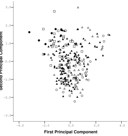
Principal Component analysis was conducted on Aegialomys sample and our results showed that first principal component accounts for 65.45% of variation, the second for 9.08% and third for 5.52% of the varia-tion (Table 11). The variables explaining the variavaria-tion along the first component are TL, CIL, and CZL, all related to the overall size of the skull. The distribution of scores between the first and second components (Fig. 4) revealed a division between specimens assigned to classes 1 and 2 and to classes 4 and 5, without clear overlap between these classes. Nevertheless, specimens identified as class 3 are predominantly overlapped to specimens from classes 2 and 4. Plotting male and female individuals on this PCA analysis (Fig. 5), it is possible to observe no clear distinction between male and female through the multivariate space.

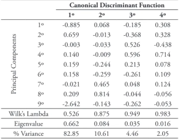
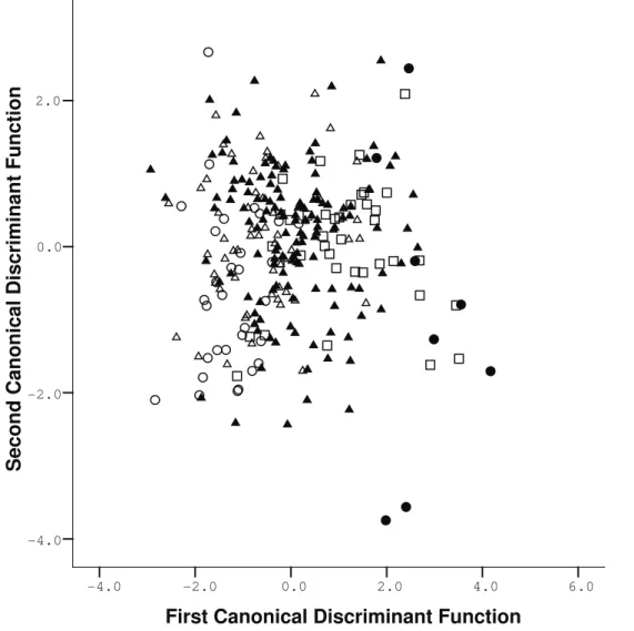
A discriminant analysis for the five age classes was performed on the Aegialomys sample, using the scores of the first nine principal components. Four Ca-nonical Functions explain the total variance; the first

is responsible for 82.85%, the second for 10.61%, the third for 4.46% and the fourth for 2.05% (Table 12). A scatterplot between the first and second canonical function (Fig. 6) evidences that specimens from class-es 1 and 2 are nclass-ested in a cloud in the right corner of the graph. Specimens assigned to classes 4 and 5 are more restricted to the left portion of the scatter plot, whereas class 3 specimens occupy an intermediate po-sition between these two major age groups. The first canonical function is influenced mainly by the first and fifth principal component, which are expressing variation on longitudinal skull size (TL, CIL, CZL) and interparietal size (BIP and LIP) of specimens ex-amined, respectively. Thus, most of the differentiation of groups is distributed along the abcissa axis of the scatterplot graph; the absence of any discriminatory power for the second function is also evident; Wilk’s Lambda shows that only the first and second canoni-cal functions exhibit statisticanoni-cal significant differences between the age classes.

DISCUSSION

Quantitative comparisons of skulls and molars have traditionally been used in systematic studies of Muroidea and these measurements promote an im-portant evidence of differences among populations (Voss, 1991), as documented in this study: we detect-ed a significant variation relatdetect-ed to age and also dif-ferences between males and females of A. xanthaeolus.

According to the univariate results described above, it seems that the age classes with minor tooth wear (1 and 2), are different among themselves and

TABLE 11: Result of Principal Component Analysis. Components that most influence the dispersion of scores are in bold.

Variable Principal Components First Second Third

TL 0.975 -0.156 -0.017 CIL 0.967 -0.167 -0.027

LD 0.935 -0.248 0.026

LM 0.670 0.558 -0.058

BM1 0.641 0.613 -0.107

LIF 0.897 0.121 -0.088

BIF 0.743 0.059 -0.058

PB 0.784 0.405 -0.069

BIP 0.557 0.190 0.443

LIP 0.266 0.098 0.883

BR2 0.892 -0.162 0.011

LN 0.947 -0.061 -0.025

LPB 0.559 -0.636 0.044

LIB 0.699 0.202 0.085

ZB 0.942 -0.137 -0.021

BZP 0.880 -0.204 -0.051

CZL 0.963 -0.197 -0.033

PFL 0.918 -0.145 -0.046

BB 0.725 0.312 -0.149

Eigenvalue 12.436 1.726 1.050 % Variance 65,45% 9,08% 5,52%

TABLE 12: Result of discriminant analysis based on the first nine principal components. Canonical Discriminant Function Coeffi-cients, Wilk’s Lambda, Eigenvalue and Variance (%) are presented.

Canonical Discriminant Function

1º 2º 3º 4º

P

rincipal Components

from all other age classes. In all analyses performed, individuals with moderate tooth wear, from class 3, are different from the adjacent age classes (2 and 4). The specimens classified as age classes 4 and 5, with intense to heavy wear, are similar in all analyses. It is noteworthy that despite the univariate analyses em-ployed (all samples pooled, males and females sepa-rated, Isla Puna sample), all results were quite similar. The multivariate results showed no significant differ-ence related to age in Isla Puna: this suggests that the evidence of significant differences provided by the in-dividual variables on univariate approach is overcome by evidence of no difference provided by all variables together on the multivariate approach. Manly (2005) stated that the use of a multivariate test as distinct from a series of univariate tests is important to control

the rates of type I error, i.e., to find a significant result when there are no differences among samples.

We believe that the major variation found in class 3 within the Aegialomys sample (in multivariate and univariate analysis) could be due to several other factors than strictly age variation (like geographic, sex, environmental, and random factors) and could be misleading: thus, the comparisons we performed (with all pooled sample) suggest that such procedures should be avoided in age or sex analysis. We interpret the age variation observed in Isla Puna in the univari-ate analysis and the absence of such variation found in the multivariate results, as resultant from sexual dimorphism detected in this sample on age class. We believe that classes 3, 4 and 5 are similar (another evidence for that: age class 3 is less different from age

class 5, than to age class 4) and could be grouped to the posterior geographic analyses.

Our results also highlight age-related differences on cranial morphology, mainly including the rostrum (BR2, LN, LD), the zygomatic region (ZB, BZP, OFL) and the overall skull size (TL, CIL).

These trends indicate a pattern of postnatal growth that we can hypothesize to occur as follows: total length of skull condylo-incisive length indicate overall skull size, and which increases at the same rate as body size. As expected from other neurocranium components, the breadth of the bulla increases follow-ing the same pattern of HB and ZB. Temporal space expands by a combination of distance outside of zy-gomatic arches and breadth of zyzy-gomatic plate, the latter growing rapidly in classes 1, 2 and 3, stabilizing afterwards. This suggests an increase in the volume of masticatory muscles in adults, due to an increase

of muscle insertion areas (ZB, BZP, OFL), especially for the temporal and masseteric muscles. Other facial skeleton dimensions (BR2, LN) show an elongation of the rostrum as the individual grows from classes 1 and 2 to classes 3, 4 and 5. On the other hand, both measurements on the molar series showed no significant variation in any age group, indicating that molars do not exhibit ontogenetic quantitative varia-tion, despite noticeable qualitative variation described above on age classes (Carleton & Musser, 1989; Voss, 1991; Giannini et al. 2009). In general, this ontoge-netic variation described for A. xanthaeolus followed the pattern described by Voss (1991) for Zygodonto-mys, and Carleton & Musser (1989) for Microryzomys.

These authors stated that the variation is larger for most craniofacial and incisors measurements, because they have indeterminate growth, revealing a general expansion of the skull as the animal grows older. On

contrary, the dimensions of molars and neurocranium are relatively less variable, which exhibit their growth early in postnatal life.

Proven sex-related differences (uni- and multi-variate) only in the total sample, lead us to consider that this result may be due to geographic variation. Nevertheless, if this is true all age classes should ex-hibit a similar pattern, and this was not observed, only age class 3 exhibited sexual dimorphism. Fur-thermore, it is interesting the result of univariate anal-ysis in Isla Puna that showed significant differences between sexes only in class 3 too (even though the multivariate analysis did not identify dimorphism in the sample).

The results of age and sex analysis show a great variation in the class 3 in A. xanthaeolus. Brandt & Pessôa (1994) also found that sexual dimorphism is

a significant factor in age class 3 of a large sample of Cerradomys langguthi from Triunfo (Pernambuco, Brazil) for seven cranial characters, and considers that sexual dimorphism may be an important source of variation where specimens of age class 3 are consid-ered. Camardella et al. (1998), evaluating a sample of C. langguthi from Viçosa and Palmeira dos Indios (Alagoas, Brazil), revealed that sexual dimorphism is not restricted to age class 3 (11 of 15 variables are di-morphic), being also observed in age classes 2, 4 and 5 (although less conspicuous; only 10 of 15, 6 of 15 and 3 of 15 variables for classes 2, 4 and 5, respectively).

It is probable that males and females indexed with tooth wear corresponding to class 3 exhibit dif-ferent growth rates: males would begin to grow larger before females, resulting in sexual differences; support-ing this assumption is the fact that in Aegialomys (and

also in C. langguthi; Brandt & Pêssoa, 1994) mature adults from age classes 4 and 5 are similar in all cra-nial measurements. It is also possible that age class 3 is inadequately defined (“First and second molar in this class with medium wear, with the cusps conspicu-ously eroded…”), thus encompassing specimens with wide range of cranial size. Another explanation could be related to dietary contents: some specimens (or specimens from a particular area, with more sand soils) could ingest more abrasive food (sometimes along with soil), resulting in relatively young individuals with advanced tooth wear (Patton & Rogers, 1983). This would increase the variation within this intermediate age class and, thus, cause confusion in the classifica-tion of age classes. Moreover, intersexual competiclassifica-tion for food and predation may cause differences in body size between males and females (Shine, 1978).

Regarding body measurements, Clark (1980) found that males were heavier and exhibited longer head and body than females in Aegialomys galapagoen-sis. A. galapagoenis also displays sexual dimorphism for skull measurements (results not show), suggest-ing that there are some degree of sexual dimorphism within the genus. Nesoryzomys swarthy, another Gala-pagos Island endemic Oryzomyini, also exhibit sexual dimorphism, accordingly to Harris & MacDonald (2007). In Galapagos, reproduction is highly sea-sonal, with males of both genera defending larger home range that encompasses home ranges of several females, suggesting high competition for receptive fe-males. Although these authors do not state it clearly, this life history will probably lead to sexual dimor-phism. It is possible that the dimorphism observed on Isla Puna sample is similar as that observed in Galapa-gos, but as data on the life history of A. xanthaeolus is lacking, we are not able to provide any insight on this subject. It is also important to establish that Isla Puna is a continental island, and shares with the continent most of its fauna (see Chapman, 1926).

The absence of sexual dimorphism and pro-nounced age-related craniometric differentiation has been reported for some Muridae rodents, including

Dasymys incomtus (Mullin et al., 2001), Aethomys chrysophilus, Micaelamys namaquensis (Chimimba & Dippenaar, 1994), and Taterillus gracilis (Robbins, 1973); for some Cricetidae rodents, as Transandino-mys talamancae (Musser & Williams, 1985), the ge-nus Microryzomys (see Carleton & Musser, 1989), the genus Zygodontomys (see Voss, 1991), several Ory-zomyini genera (Musser et al., 1998), and the genus

Cerradomys (see Percequillo et al., 2008), and for Pro-echimys brevicauda from family Echimyidae (Patton & Rogers, 1983).

On the other hand, information available re-garding the Akodontini tribe highlighted the exis-tence of sexual dimorphism, even though it is not in all age groups (Macêdo & Mares, 1987; Oliveira, 1992). However, Ventura et al. (2000), evaluating several akodontine morphotypes, did not detect this type of variation. Within the Oryzomyini tribe, sexual dimorphism is a conspicuous feature in some skull characters of the genus Oligoryzomys, such as O. ni-gripes, O. chacoensis and O. fornesi (Myers & Carleton, 1981), and in some insular populations of Aegialomys

(this study; Clark, 1980) and Cerradomys (Brandt & Pêssoa, 1994; Carmadella et al., 1998). As the sexual variation observed in A. xanthaeolus is not consistent (sexual dimorphism was observed only in Isla Puna and in Aegialomys sample, which probably also in-cludes geographic variation), we will pool both sexes to assess geographic variation throughout mainland sam-ples and clusters; for insular populations we will keep males and females separated for all subsequent analysis.

CONCLUSION

Evaluating the non-geographic variation within

Aegialomys xantaheolus, allowed us to assert that, re-garding the samples available and cranial traits ana-lyzed, sexual dimorphism is an important component of variation in class 3 for some samples of this species, differing from most taxa of the tribe Oryzomyini, in which morphometric studies found only a minor or negligible sexual variation in the measured variables. Nevertheless, considering the variation described here regarding age variation and sexual dimorphism, we recommend that non-geographic analysis should be performed as part of the protocol in morphometrical studies on sigmodontine rodents.

RESUMO

delimitação de táxons. Este trabalho representa um estudo inicial com A. xanthaeolus, sumarizando a informação existente a respeito da sua distribuição geográfica e com-preendendo sua variação relacionada ao sexo e à idade. Para tal nos baseamos nas análises de mensuração morfo-métrica tradicional de 19 medidas crânio-dentárias aces-sadas em coleções científicas, e organizamos as localidades de coleta dos espécimes examinados em um índice de lo-calidades e um mapa de distribuição. A análise dos dados teve uma abordagem morfológica em nível quantitativo, através de análises estatísticas uni e multivariadas. Os resultados obtidos nos permitem afirmar que a variação ontogenética é significante, que as classes etárias 3, 4 e 5 podem ser agrupadas para as análises de variação geo-gráfica e que o dimorfismo sexual não é um componente consistente de variação para esta espécie, quando conside-ramos amostras provenientes de uma mesma localidade, ou de localidades próximas umas as outras.

Palavras-Chaves: Distribuição Geográfica; Crânio; Ontogenia; Dimorfismo sexual.

ACKNOWLEDGEMENTS

We thank the curators of the museums visited, Dr. Robert Voss (American Museum of Natural His-tory, New York); Dr. James L. Patton (Museum of Vertebrate Zoology, Berkeley); Dr. Mark S. Hafner (Museum of Zoology, Louisiana State University); Dr. Michael Carleton (Smithsonian Institution, National Museum of Natural History); Dr. Bruce Patterson (The Field Museum, Chicago); Dr. Paula Jenkins (The Natural History Museum, London); Dr. Phil Myers (University of Michigan, Museum of Zoology, Ann Arbor). ARP also would like to thanks Dr. Mario de Vivo for his support and encouragement during his doctorate studies. We also would like to acknowledge to two anonymous reviewers that greatly contributed to the improvement of the manuscript. This contribu-tion was supported by Fundação de Amparo à Pesquisa do Estado de São Paulo (FAPESP 1998/12273-0, Pro-grama Biota 1998/05075-7; FAPESP 2009/03547-5; FAPESP JP 2009/16009-1) and CNPq (2008/476249) and grants from the American Museum of Natural History, the Field Museum, the Smithsonian Institu-tion, the Museum of Comparative Zoology.

REFERENCES

Abdel-Rahman, E.H.; Taylor, P.J.; Contrafatto, G.; Lamb, J.M.; Bloomer, P. & Chimimba, C.T. 2008. Geometric craniometric

analysis of sexual dimorphism and ontogenetic variation: A case study based on two geographically disparate species, Aethomys ineptus from southern Africa and Arvicanthis niloticus from Sudan (Rodentia: Muridae). Mammalian Biology, 74:361-373. Brandt, R.S. & Pêssoa, L.M. 1994. Intrapopulacional variability

in cranial characteres of Oryzomys subflavus (Wagner, 1842) (Rodentia: Cicretidae), in northeastern Brazil. Zoologischer An-zeiger, 233:45-55.

Cabrera, A. 1961. Catalogo de los Mamiferos de America del Sur.

Revista del Museo Argentino de Ciencias Naturales “Bernadino Rivadavia”, 4(part 2):309-732.

Carleton, M.D. & Musser, G.G. 1989. Systematic studies of oryzomyine rodents (Muridae, Sigmodontidae): a synopsis of Microryzomys. Bulletin of the American Museum of Natural History, 191:1-83.

Carmadella, A.R.; Pessôa, L.M. & Oliveira, J.A. 1998. Sexual dimorphism and age variability in cranial characters of

Oryzomys subflavus (Wagner, 1842) (Rodentia: Sigmodontinae) from northeastern Brazil. Bonner Zoologische Beiträge, 48:9-18. Chapman, F.M. 1926. The distribution of bird-life in Ecuador:

a contribution to a study of the origin of Andean bird-life.

Bulletin of the American Museum of Natural History, 55:1-784. Chimimba, C.T. & Dippenaar, N.J. 1994. Non-geographic

variation in Aethomys chrysophilus (De Winton, 1897) and

A. namaquensis (A. Smith, 1834) (Rodentia: Muridae) from southern Africa. South African Journal of Zoology, 29:107-117. Clark, D. 1980. Population ecology of an endemic neotropical

island rodent: Oryzomys bauri of Santa Fe Island, Galapagos, Ecuador. Journal of Animal Ecology, 49:185-198.

Gardner, A.L. & Patton, J.L. 1976. Karyotypic variation in oryzomyine rodents (Cricetidae) with comments on chromosomal evolution in the neotropical cricetinae complex.

Occasional Pappers Lousiana State University Museum of Zoology, 49:1-48.

Giannini, N.P.; Segura, V.; Giannini, M.I. & Flores, D. 2009. A quantitative approach to the cranial ontogeny of the puma.

Mammalian Biology, 75:547-554.

Harris, D.B. & Macdonald, D.W. 2007. Population ecology of the endemic rodent Nesoryzomys swarthy in the Tropical desert of the Galapagos Islands. Journal of Mammalogy, 88:208-219. Heller, E. 1904. Mammals of the Galapagos Archipelago,

exclusive of the Cetacea. Proceedings of the California Academy of Sciences, 3:223-251.

Johnson, R.A. & Wichern, D.W. 1999. Applied multivariate statistical analysis. Upper Saddle River, New Jersey.

Kankainen, A.; Taskinen, S. & Oja, H. 2003. On Mardia’s Tests of Multinormality. Statistical Methods and Applications,

16:357-379.

Macêdo, R.H. & Mares, M.A. 1987. Geographic variation in the South American cricetine rodent Bolomys lasiurus. Journal of Mammalogy, 68:578-594.

Manly, B.F.J. 2005. Multivariate Statistical Methods: A Primer. Chapman & Hall/CRC, New York.

Mayr, E. 1969. Principles of Systematic Zoology. McGraw-Hill Inc., New York.

Mayr, E. 1977. Populações, espécies e evolução. Ed. Nacional, EDUSP, São Paulo.

Mullin, S.K.; Pillay, N. & Taylor, P.J. 2001. Non-geographic morphometric variation in the water rat Dasymys incomtus

(Rodentia: Muridae) in southern Africa. Durban Museum Novitates, 26:38-44.

Musser, G.G. & Williams, M.M. 1985. Systematic Studies of Oryzomyine Rodents (Muridae): definitions of Oryzomys talamancae. American Museum Novitates, 2810:1-22. Musser, G.G.; Carleton, M.D.; Brothers, E. & Gardner, A.L.

1998. Systematic studies of Oryzomyine rodents (Muridae, Sigmodontinae): diagnoses and distributions of species formerly assigned to Oryzomys “capito”. Bulletin of the American Museum of Natural History, 236:1-376.

Myers, P. & Carleton, M.D. 1981. The Species of Oryzomys (Oligoryzomys) in Paraguay and the Identity of Azara’s “Rat sixieme ou Rat a Tarse Noir”. Miscellaneous Publications Museum of Zoology, University of Michigan, 161:1-41.

Oliveira, J.A. de. 1992. Estrutura da variação craniana em populações de Bolomys lasiurus (Lund, 1841) (Rodentia: Cricetidae) do nordeste do Brasil. (Dissertação de Mestrado). Universidade Federal do Rio de Janeiro, Rio de Janeiro. Patton, J.L. & Hafner, M.S. 1983. Biosystematics of the native

rodents of the Galapagos Archipelago, Ecuador. In: Bow-man, R.I.; Berson, M. & Leviton, A.E., Patterns of evolution in Galapagos organisms. AAAS Pacific Division, San Francisco, p.539-568.

Patton, J.L. & Rogers, M.A. 1983. Systematic implications of non-geographic variation in the spiny rat genus Proechimys

(Echimyidae). Mammalian Biology, 48:363-370.

Paynter Jr., R.A. 1993. Ornithological Gazetteer of Ecuador. Bird Department, Museum of Comparative Zoology, Harvard University, Cambridge.

Percequillo, A.R. 1998. Sistemática de Oryzomys Baird, 1858 do leste do Brasil (Muroidea, Sigmodontinae). (Dissertação de Mestrado). Universidade de São Paulo, São Paulo.

Percequillo, A.R. 2003. Sistemática de Oryzomys Baird, 1858: definição dos grupos de espécies e revisão do grupo albigularis (Rodentia, Sigmodontinae). (Tese de Doutorado). Universidade de São Paulo, São Paulo.

Percequillo, A.R., Hingst-Zaher, E. & Bonvicino, C.R. 2008. Systematic review of genus Cerradomys Weksler, Percequillo and Voss, 2006 (Rodentia: Cricetidae: Sigmodontinae: Oryzomyini), with description of two new species from Eastern Brazil. American Museum novitiates, 3622:1-46. Reis, S.F.; Duarte, L.C.; Monteiro, L.R. & von Zuben, F.J. 2002.

Geographic variation in cranial morphology in Thrichomys apereoides (Rodentia:Echimyidae). I. Geometric descriptors and patterns of variation in shape. Journal of Mammalogy,

83:333-344.

Reis, S.F.; Pêssoa, L.M. & Straus, R.E. 1990. Application of size-free canonical discriminant analysis to studies of geographic differentiation. Revista Brasileira de Genética, 13:509-520. Robbins, C.B. 1973. Non-geographic variation in Taterillus gracilis

(Thomas) (Rodentia: Cricetidae). Journal of Mammalogy,

54:222-238.

Shine, R. 1978. Sexual size dimorphism and male combat in snakes. Oecologia, 33:269-277.

Sokal, R.R. & Rohlf, F.J. 1997. Biometry. W.H. Freeman and Company, New York.

Stephens, L. & Traylor, M.A. Jr. 1983. Ornithological Gazetteer of Peru. Bird Department, Museum of Comparative Zoology, Harvard University, Cambridge.

Thomas, O. 1894. Descriptions of some new Neotropical Muridae.

Annals and Museum of Natural History, 14:346-366.

Thorpe, R.S. 1976. Biometric analysis of geographic variation and racial affinities. Biological reviews, 51:407-452.

Ventura, J.; López-Fuster, M.J.; Salazar, M. & Pérez-Hernández, R. 2000. Morphometric analysis of some Venezuelan akodontine rodents. Netherlands Journal of Zoology, 50:487-501. Voss, R. S. 1988. Systematics and ecology of Ichthyomyine rodents

(Muroidea): patterns of morphological evolution in a small adaptive radiation. Bulletin of the American Museum of Natural History, 188(2): 259-493.

Voss, R.S. 1991. An introduction to the Neotropical muroid rodent genus Zygotontomys. Bulletin American Museum of Natural History, 210:1-113.

Weckerly, F.W. 1998. Sexual-size dimorphism: influence of mass and mating system in the most dimorphic mammals. Journal of Mammalogy, 79:33-52.

Weksler, M. 2003. Phylogeny of neotropical oryzomyine rodents (Muridae:Sigmodontinae) based on the nuclear IRBP exon.

Molecular Phylogenetics and Evolution, 29:331-349.

Weksler, M. 2006. Phylogenetic relationships of oryzomyine rodents (Muroidea: Sigmodontinae): separate and combined analyses of morphological and molecular data. Bulletin of the American Museum of Natural History, 296:1-149.

Weksler, M.; Percequillo, A.R. & Voss, R.S. 2006. Ten New Genera of Oryzomyine Rodents (Cricetidae: Sigmodontinae).

American Museum Novitates, 3537:1-29.

APPENDIX A

Material Examined

APPENDIX B

Aegialomys xanthaeolus (Thomas, 1894)

Gazetteer

Ecuador

El Oro

1. 12 km E by road Portovelo [ca. 792 m]. Not located; here are employed the geographical coordinates of Portovelo. 03°20’S, 79°49’W.

2. Pasage [ca. 61 m]. 03°20’S, 79°49’W. 3. Portovelo [ca. 610 m]. 03°43’S, 79°39’W.

4. Rio Pindo, Portovelo [ca. 564 m]. 03°50’S, 79°45’W. 5. Santa Rosa [ca. 31 m]. 03°27’S, 79°58’W.

Esmeraldas

6. Esmeraldas [sea level]. 00°59’N, 79°42’W.

Guayas

7. Cerro Manglaralto, Santa Elena (part of Sierra de Colonche) [ca. 365 m]. Not located; here are employed the geographical coordinates of Colonche. 02°00’S, 80°20’W.

8. Chongoncito, Guayaquil [ca. 365 m]. 02°14’S, 80°05’W.

9. Huerta Negra, 20 km ESE Balao, east of Tenguel. 03°00’S, 79°46’W. 10. Isla Puna, San Ramon, Guayaquil [ca. 925 m]. 02°50’S, 80°08’W. 11. Rio Chongón. 1.5 km SE Chongón [ca. 70 m]. 02°14’S, 80°4’W. 12. San Rafael, 7 km S Balao. 03°59’S, 79°47’W.

Loja

13. Alamor, San Agustin, Puyango [ca. 1325 m]. 04°02’S, 80°02’W. 14. Amaluza. 04°36’S, 79°25’W.

15. Casanga River Valley [ca. 875 m]. Not located; here are employed the geographical coordinates of Rio Ca-sanga. 04°08’S, 79°49’W.

16. Catacocho, Olmedo, Paltas [1872 m]. 04°04’S, 79°38’W. 17. Hacienda Casanga, Paltas [884 m]. 04°01’S, 79°45’W.

18. Jatumpamba (used the coordinates of Jatum Pamba). 04°16’S, 79°42’W. 19. Loja. 04°00’S, 79°13’W.

20. Los Pozos, Macara. 04°23’S, 79°57’W. 21. Malacatos. 04°14’S, 79°15’W.

22. Sabiango, La Caprilla. 04°24’S, 79°52’W.

Los Rios

24. Hacienda Pijigual, Vinces. Not located; here are employed the geographical coordinates of Vinces. 01°32’S, 79°45’W.

25. Hacienda Santa Teresita (Abras de Mantequilla), ca. 12 km NE Vinces. Not located; here are employed the geographical coordinates of Vinces. Aegialomys xanthaeolus, 01°32’S, 79°45’W.

26. Vinces, near Puerto Nuevo and Vinces. 01°32’S, 79°45’W.

Manabí

27. Cuaque, Pedernales [sea level]. 00°00’S, 80°06’W.

28. Hacienda San Carlos, Bahia de Caraquez, Rio Briseño, Sucre [sea level]. 00°36’S, 80°25’W.

Pichincha

29. Great Quito Railroad, Kilometer 8. Not located; here are employed the geographical coordinates of Quito. 00°13’S, 78°30’W.

Peru

Amazonas

30. 8 km WSW Bagua [ca. 457 m]. 05°40’S, 78°31’W. 31. Balsas, Chachapoyas [ca. 854 m]. 06°50’S, 78°01’W.

Ancash

32. 1 km N, 12 km E of Pariacoto [ca. 2590 m]. 09°31’S, 77°53’W.

33. 4 km by road NE Chasquitambo, km 51. Not located; here are employed the geographical coordinates of Chasquitambo. 13°48’S, 73°23’W.

34. Chasquitambo, Julcan. 10°18’S, 77°36’W. 35. Macate, Santa [ca. 2712 m]. 08°46’S, 78°05’W. 36. Pariacoto, Huaraz [ca. 1239 m]. 09°32’S, 77°32’W.

Arequipa

37. 41/2 mi. E Acari. Not located; here are employed the geographical coordinates of Acari. 15°26’S, 74°37’W. 38. 81/2 mi. NNW Bella Union [ca. 731 m]. Not located; here are employed the geographical coordinates of

Bella Union. 15°26’S, 74°39’W.

39. Chavina, on the coast near Acari, Rio Lomos, Province Caravelli. 15°37’S, 74°38’W.

Cajamarca

40. Cascas [ca. 1274 m]. 07°29’S, 78°49’W.

41. El Arenal, Rio Huancabamba, 7 km, 50 km E, Olmos [ca. 915 m]. 05°59’S, 79°46’W. 42. Hacienda Limon, Celendin [ca. 2048 m]. 06°50’S, 78°05’W.

Huanuco

45. Hacienda Buena Vista, Chinchao [ca. 1066 m]. Not located; here are employed the geographical coordi-nates of Chinchao. 09°38’S, 76°04’W.

Ica

46. Hacienda San Jacinto, Ica. 14°09’S, 75°45’W.

47. Hacienda San Pablo, El Ingenio, 30 km Nazca. Not located; here are employed the geographical coordinates of El Ingenio. 14°39’S, 75°05’W.

48. San Javier, 13 km S Palpa [ca. 275 m]. 14°32’S, 75°11’W.

La Libertad

49. 5 km NE Pacasmayo [ca. 61 m]. 07°24’S, 79°34’W. 50. Menocucho, Trujillo [ca. 500 m]. 08°01’S, 78°50’W. 51. Pacasmayo [ca. 8 m]. 07°24’S, 79°34’W.

52. Trujillo [ca. 34 m]. 08°07’S, 79°02’W.

Lambayeque

53. 2 km W Porculla Pass [ca. 1981 m]. Not located; here are employed the geographical coordinates of Por-culla Pass. 05°51’S, 79°31’W.

54. 7.5 km N of Olmos [ca. 304 m]. Not located; here are employed the geographical coordinates of Olmos. 05°59’S, 79°46’W.

55. 8 km S Morrope [ca. 304 m]. Not located; here are employed the geographical coordinates of Morrope. 06°33’S, 80°01’W.

56. 12 mi. ENE Olmos [ca. 610 m]. Not located; here are employed the geographical coordinates of Olmos. 50°59’S, 79°46’W.

57. Chongoyape, Chiclayo [ca. 209 m]. 06°46’S, 79°51’W. 58. Hacienda El Carmen, Motupe [ca. 130 m]. 06°09’S, 79°44’W. 59. Olmos [ca. 175 m]. 05°59’S, 79°46’W.

Lima

60. 7 km SSE Chilca [ca. 2 m]. Not located; here are employed the geographical coordinates of Chilca. 12°32’S, 76°44’W.

61. 8 km SE Chilca [ca. 150 m]. Not located; here are employed the geographical coordinates of Chilca. 12°32’S, 76°44’W.

62. 10 km ENE Pucusana [ca. 250 m]. Not located; here are employed the geographical coordinates of Pu-cusana. 12°29’S, 76°48’W.

63. 1 mi. W Matucana [ca. 1981 m]. Not located; here are employed the geographical coordinates of Matu-cana. 11°51’S, 76°24’W.

64. 1 mi. W Surco [ca. 1828 m]. Not located; here are employed the geographical coordinates of Surco. 11°52’S, 76°28’W.

65. 5 mi. E Yanyos [ca. 2743 m]. Not located.

68. Hacienda Casa Blanca, Cerro del Oro, Canete. Not located; here are employed the geographical coordinates of Canete. 13°04’S, 76°23’W.

69. Lima [ca. 154 m]. 12°03’S, 77°03’W.

70. Lomas de Lachay, 22 km N, 11 km W of Cancay [ca. 396 m]. 11°21’S, 77°23’W. 71. Loma Viscachera. 12°31’S, 76°30’W.

72. Santa Eulalia [ca. 1036 m]. 11°51’S, 76°41’W.

73. Santa Eulalia Cyn, 6 mi. NNE Chosica. Not located; here are employed the geographical coordinates of Santa Eulalia. 11°51’S, 76°41’W.

74. Tornamesa. 11°54’S, 76°31’W. 75. Vitarte. 12°02’S, 76°56’W.

Piura

76. Catacaos. 05°16’S, 80°41’W.

77. Hacienda Bigotes, Morropon [ca. 200 m]. 05°19’S, 79°48’W. 78. Hacienda Mallares, Sullana. 04°53’S, 80°41’W.

79. Hacienda San Luis, La Arena. Not located; here are employed the geographical coordinates of La Arena. 05°20’S, 80°44’W.

80. Huancabamba [ca. 1929 m]. 05°14’S, 79°28’W. 81. Laguna [ca. 1150 m]. 04°41’S, 79°50’W. 82. Lancones, Sullana. 04°35’S, 80°30’W.

83. Las Trancas, Cerro Cortezo, Sullana. 04°53’S, 80°41’W.

84. Monte Grande, 14 km N, 25 km E of Talara. 04°28’S, 81°03’W.

85. Paymas, Ayabaca [ca. 700 m]. Coordenates of Ayabaca. 04°38’S, 79°43’W. 86. Piura [ca. 50 m]. 05°12’S, 80°38’W.

Tumbez

87. El Sauce. 07°06’S, 79°19’W.

88. Matapalo, Zarumilla [ca. 54 m]. 03°41’S, 80°12’W. 89. Positos, Zarumilla [ca. 25 m]. 04°16’S, 80°30’W.