SPATIO-TEMPORAL PATTERN MINING FROM GLOBAL
POSITIONING SYSTEMS (GPS) TRAJECTORIES DATASET
ii
SPATIO-TEMPORAL PATTERN MINING FROM GLOBAL POSITIONING
SYSTEMS (GPS) TRAJECTORIES DATASET
Dissertation supervised by:
Supervisor:
Prof. Dr. Edzer Pebesma, Institute for Geoinformatics, University of Muenster, Germany
Co-supervisors:
Prof. Dr. Oscar Belmote, Institute of New Imaging Technologies, Universitat Jaume I, Spain
Prof. Dr. Roberto Henriques, Universidade NOVA de Lisboa, Portugal
iii
DECLERATION OF ORIGINALITY
I declare that this thesis is my original work and has not been presented for a degree in any other university.
iv
ACKNOWLEDGMENTS
First and foremost extraordinary thanks go for my Almighty God and His Mother Saint-Merry.
It is with immense gratitude that I acknowledge the support and help of my supervisor, Prof. Dr. Edzer Pebesma. His patience, advises and support helped me overcome challenging situations and finish this thesis. It gives me great pleasure in acknowledging the support and help of my co-supervisors Prof. Dr. Oscar Belmote and Prof. Dr. Roberto Henriques.
I would like to thank all lecturers, staff members and classmates of Geospatial Technologies for their contribution in the special arena for the success of my study. I have to give a special mention for the program coordinator Dr. Christoph Brox. I have no word to express my feeling for his endless help and support during my good and worst times. I am also thankful to course coordinators Dori A. and Karsten H. who have helped me a lot during my study.
I would like to thank the European Commission for funding my study and gave me a great opportunity to explore lots of cultures in Europe.
Most importantly, none of these would have been possible without the love and patience of my father and my mother. In the meantime, I would like to express my heart-felt gratefulness to my beloved wife, Meazashwork Assefa, who has been a continuous source of love, concern, support and strength all the times.
v
SPATIO-TEMPORAL PATTERN MINING FROM GLOBAL POSITIONING SYSTEMS (GPS) TRAJECTORIES DATASET
ABSTRACT
The increasing frequency of use location-acquisition technology like the Global Positioning
System is leading to the collection of large spatio-temporal datasets. The prospect of discovering
usable knowledge about movement behavior, which encourages for the discovery of interesting
relationships and characteristics users that may exist implicitly in spatial databases. Therefore
spatial data mining is emerging as a novel area of research.
In this study, the experiments were conducted following the Knowledge Discovery in Database
process model. The Knowledge Discovery in Database process model starts from selection of the
datasets. The GPS trajectory dataset for this research collected from Microsoft Research Asia
Geolife project. After taking the data, it has been preprocessed. The major preprocessing
activities include:
Fill in missed values and remove outliers;
Resolve inconsistencies, integration of data that contains both labeled and unlabeled datasets,
Dimensionality reduction, size reduction and data transformation activity like discretization tasks were done for this study.
A total of 4,273 trajectory dataset are used for training the models. For validating the
performance of the selected model a separate 1,018 records are used as a testing set. For building
a spatiotemporal model of this study the K-nearest Neighbors (KNN), decision tree and Bayes
algorithms have been tasted as supervised approach.
The model that was created using 10-fold cross validation with K value 11 and other default
parameter values showed the best classification accuracy. The model has a prediction accuracy
of 98.5% on the training datasets and 93.12% on the test dataset to classify the new instances as
bike, bus, car, subway, train and walk classes. The findings of this study have shown that the
spatiotemporal data mining methods help to classify user mobility transportation modes. Future
vi
TABLE OF CONTENTS
DECLERATION OF ORIGINALITY ... iii
ACKNOWLEDGMENTS ... iv
ABSTRACT ... v
TABLE OF CONTENTS... vi
KEYWORDS ...viii
ACRONYMS ... ix
INDEX OF TABLES ... x
INDEX OF FIGURES ... xi
CHAPTER 1 ... 1
INTRODUCTION ... 1
1.1. Background ... 1
1.2. Statement of the Problem ... 2
1.3. Objective of the Study ... 2
1.3.1. General Objective ... 2
1.3.2. Specific Objectives ... 2
1.4. Methodology of the Study ... 3
1.4.1. Data Collection ... 3
1.4.2. System Design and Data Preprocessing ... 3
1.4.3. Implementation tool ... 4
1.5. Organization of the thesis ... 4
CHAPTER 2 ... 5
LITERATURE REVIEW ... 5
2.1. Spatio-temporal Data Mining and Knowledge Discovery ... 5
2.2. Spatial Data Mining Models ... 5
2.2.1. The KDD Process Model ... 6
2.2.2. The CRISP- DM Process ... 7
2.2.3. Comparison of Different Spatial Data Mining Models ... 9
2.3. Spatio-temporal Data Mining Tasks ... 10
vii
2.3.2. Predictive Model ... 13
2.4. Application of Spatial Data Mining ... 19
2.5. Related Works on Spatial-temporal pattern mining for transportation modes discovery from GPS trajectories ... 21
CHAPTER 3 ... 23
METHODOLOGY AND EXPERIMENTAL DESIGN ... 23
3.1. Data Description ... 23
3.2. Initial Data Selection... 24
3.3. Data Cleaning and preprocessing ... 25
3.4. Evaluation Metrics ... 26
3.4.1. Error Rate ... 26
3.4.2. Accuracy ... 26
3.4.3: Precision and Recall ... 26
3.5. Experimentation... 27
3.5.1. Experimentation Design ... 27
3.5.2. Train the classifier using KNN Algorithm ... 28
3.5.3. Train the classifier using J48 decision tree modeling ... 35
3.5.4. Train the classifier using Naive Bayes modeling ... 36
3.5.4: Comparison of Supervised Approaches: J48 decision tree, Naive Bayes model and KNN ... 36
CHAPTER 4 ... 38
RESULTS AND DISCUSSION ... 38
CHAPTER 5 ... 43
CONCLUSION AND FUTURE WORKS ... 43
5.1. CONCLUSION ... 43
5.2. FUTURE WORKS ... 44
REFERENCES... 45
viii
KEYWORDS
Accuracy
Cross Validation
Data Mining
Geo-life
GPS
K-Nearest-Neighbor
Trajectory
Transportation modes
ix
ACRONYMS
AI- Artificial Intelligence
ANN- Artificial Neural Networks
ARFF- Attribute-Relation File Format
BN- Bayesian Network
CRISP-DM- Cross Industry Standard Process for Data Mining
CSV- Comma Separated Value
DM - Data Mining
FN- True Negative
FP - False Positive
GIS- Geographic Information System
GPS- Global Positioning System
KDD- Knowledge discovery in Database
KNN - K-Nearest-Neighbor
LVQ - Learning Vector Quantization
LWL- Locally Weighted Learning
OCA- Overall Classification accuracy
SVM- Support vector machine
TN- True Negative
TP- True Positive
x
INDEX OF TABLES
Table 2.1: Comparison of DM and KD process models and methodologies……….10
Table 3.1: Distribution of datasets ………25
Table 3.2: Exemplifier to compute recall and precision accuracy………27
Table 3.3: Classification accuracy using K value 1 ………..28
Table 3.4: Classification accuracy for each modes of transportation with k=1 ………….……..29
Table 3.5: Classification accuracy using K value 2 ………..30
Table 3.6: Classification accuracy for each modes of transportation with k=2 ………...30
Table 3.7: Classification accuracy using K value 5 ………..30
Table 3.8: Classification accuracy for each modes of transportation with k=5 ………...31
Table 3.9: Classification accuracy using K value 10 ………....31
Table 3.10: Classification accuracy for each modes of transportation with k=10 ………...31
Table 3.11: Classification accuracy using K value 11 ………..32
Table 3.12: Classification accuracy for each modes of transportation with k=10 ………...32
Table 3.13: Classification accuracy using K value 12 ………..32
Table 3.14: Classification accuracy using K value 15 ………..33 Table 3.15: Classification accuracy using K value 20 ………..33
Table 3.16: Classification accuracy using K value 30 ………..34
Table 3.17: Classification accuracy using K value 30 ………..34
Table 3.18: Some of the J48 algorithm parameters and their default values ………....35
Table 3.19: Using J48 algorithm parameters with 10-fold cross validation ……….35
Table 3.20: Classification accuracy using Naïve Bayes algorithm ………..36
Table 3.21: Comparison of Supervised Approaches ………36
Table 4.1: Results of classification accuracy with different K values ………..39
Table 4.2: Average TP and FP Rates ………39
Table 4.3: Classification result of unlabeled datasets based on the selected model ……….41
xi
INDEX OF FIGURES
Figure 1.1: An overview of the steps that compose the KDD process ………...4
Figure 2.1: KDD process: “From Knowledge Discovery to Data Mining” ………7
Figure 2.2: CRISP-DM process model ………..8
Figure 2.3: Schematic representation of the neural network model ……….16
Figure 2.4: The structure of Bayes network ………..17
Figure 2.5: Simple example of SVM ………...18
Figure: 4.1: Results of classification accuracy with different K-values ………..39
Figure 4.2: True Positive (TP) rate comparison of different K-values……….40
CHAPTER 1
INTRODUCTION
1.1. Background
Geographic and temporal properties are a key aspect of many data analysis problems in business,
government, and science. Through the availability of cheap sensor devices we have witnessed an
exponential growth of geo-tagged data in the last few years resulting in the availability of
fine-grained geographic data at small temporal sampling intervals [1]. Therefore, the actual challenge
in geo-temporal analysis is moving from acquiring the right data towards large-scale analysis of
the available data.
Many data mining techniques were originally targeted towards simple structured datasets such as
relational databases or structured data warehouses. More importantly these algorithms were used
to classify data that occur in the same time period or in other words, those datasets that are not
expected to change much over time. However, technological improvements and the internet have
led to more sophisticated data collection methods thus resulting in more complex data systems
such as multimedia, spatial and temporal databases which unstructured or semi-structured [30].
Spatio-temporal data mining is a process of generating new patterns from the existed data based
on the spatial and temporal information [1]. As discussed by [1] Spatio-temporal data mining is
a subfield of data mining which gained high popularity especially in geographic information
sciences due to the pervasiveness of all kinds of location-based or environmental devices that
record position, time or/and environmental properties of an object or set of objects in real-time.
The increasing availability of large-scale trajectory data provides us great opportunity to explore
them for knowledge discovery in transportation systems using advanced data mining techniques
[9]. As a consequence, different types and large amounts of spatio-temporal data became
available those introduce new challenges to data analysis and require novel approaches to
2 1.2. Statement of the Problem
With the help of various positioning tools, individuals’ mobility behaviors are being
continuously captured from mobile phones, wireless networking devices and Global positioning
system (GPS) appliances [6]. These mobility data serve as an important foundation for
understanding individuals’ mobility behaviors. As discussed by [6] the dissimilarity in the mobility areas covered by individuals, there is high regularity in the human mobility behaviors,
suggesting that most individuals follow a simple and reproducible pattern.
In the current technology users are used to navigate using different GPS technologies. But it is
challenging to uncover mobility patterns from GPS datasets. It is important predicting the future
moves, detecting modes of transport, mining trajectory patterns and recognizing location based
activities.
Using the GPS trajectory dataset it is possible to monitor the behavior of traffic. For example we
can use GPS data from cars or other transportation modes to monitor the emergence of
unexpected behavior in the given region. Knowing the pattern has the potential to estimate and
improve traffic conditions in advance and will reduce
emerging anomalous.
This research intends to get answers for the following research questions:
What are the patterns to categorize users’ transportation modes behavior form GPS logs?
What are the ways used for detecting mode of transport for user navigation using GPS?
Which machine learning algorithm will achieve a better result in the supervised approach for GPS trajectories?
1.3. Objective of the Study
1.3.1. General Objective
The general objective of this study is to develop Spatio-temporal model for user transportation
mode from the GPS trajectories data.
1.3.2. Specific Objectives
The specific objectives of this study are the following:
3
to develop supervised model for user mobility modes.
to detect modes of transport based on machine learning Algorithms.
to select the better machine leaning algorithm for Spatio-temporal trajectory dataset.
1.4. Methodology of the Study
1.4.1. Data Collection
The GPS trajectory dataset for this research collected from Microsoft Research Asia Geolife
project by a group of users in a period of over three years (from April 2007 to August 2012) [2]
[3] [4] [5]. A GPS trajectory of this dataset is represented by a sequence of time-stamped points,
each of which contains the information oflatitude, longitude and altitude.
1.4.2. System Design and Data Preprocessing
For this study a combination of data mining tasks and spatial data representation were applied.
For identifying users’ behavior data mining tasks like supervised algorithms were applied.
Data processing, a critical initial step in data mining work, is often used to improve the quality of
training data set. To do so data cleaning and preparation is the core task of data mining which is
dependent on software chosen and algorithms used [8].
The data mining model used in this study is the Knowledge discovery in Database (KDD)
process. The KDD process refers to the whole process of changing low level data into high level
knowledge which is automated discovery of patterns and relationships in large databases and
data mining is one of the core steps in the KDD process. The goal of KDD and Data Mining
(DM) is to find interesting patterns and/or models that exist in databases but are hidden among
the volumes of data [7]. The KDD process as described by [7] consists of five major phases.
Data will collect then using appropriate algorithms then mined patterns will be modeled. Figure
4
Figure 1.1: An overview of the steps that compose the KDD process [7].
1.4.3. Implementation tool
The research was conducted using DM software packages (Weak tool and Tanagra) and other
necessary tools (like Microsoft excel) to identify the transportation modes pattern. Disk
Operating System (DOS) and Java Command line interface used for testing the model using
unlabeled datasets.
1.5. Organization of the thesis
This thesis is structured into five chapters. The first chapter discusses background to the study
problem area, statement of the problem, objective of the study and research methodology.
The second chapter discusses about DM and knowledge discovery technology, DM Processes,
DM models, application of DM in general and in particular in the area of Spatio-temporal data
mining for transportation modes.
The third chapter deals with understanding the data and dataset preparation, Data transformation
and experimentations
The fourth chapter provides a comprehensive results and discussion of the experiential results.
5
CHAPTER 2
LITERATURE REVIEW
The researcher has reviewed different related literatures (books, journal articles, conference
proceeding papers, and the Internet) in order to have detailed understanding on the present
research.
2.1. Spatio-temporal Data Mining and Knowledge Discovery
Spatial data records information regarding the location, shape and its effect on features (e.g.
geographical features). When such a data is time variant, it is called spatiotemporal data.
Spatio-temporal data mining is an upcoming research topic which focuses on studying and
implementing novel computational techniques for large scale spatiotemporal data [31]. Progress
in hardware technologies such as portable display devices, wireless devices has enabled an
increase in availability of location-based services. In addition, GPS data is becoming
increasingly available and accurate. These developments pave way to a range of new
spatio-temporal applications such as distributed systems, location based advertising, disease
monitoring, real estate process etc. Having explored temporal data mining, the next step is to
extend data mining techniques to spatiotemporal data. This is because in most cases, the spatial
and temporal information is implicitly present in the databases; it might be either metric-based
(e.g. size) or non-metric based (e.g. terrain, storm path) or both. It is therefore necessary to
acknowledge it before carrying out data mining processes that target developing real time
models. The spatial and temporal dependencies are inherently present in any spatio-temporal
databases. Spatio-temporal data mining can thus be defined as identifying the interesting and
non-trivial knowledge from large amounts of spatio-temporal data. Spatio-temporal data mining
applications range from transportation, remote sensing, satellite telemetry, monitoring
environmental resources and geographic information systems (GISs) [31]
2.2. Spatial Data Mining Models
Temporal data mining is often carried out with one of the following intentions; predictions,
classification, clustering, search and pattern identification [34]. Early predictive models assumed
6
intelligence (AI) modeling were employed to develop non linear temporal modeling. Clustering
in time series data provides an opportunity to understand it at a higher level of abstraction by
studying the characteristics of the grouped data. Temporal data clustering has numerous
applications ranging from understanding protein structure to learn and characterize financial
transactions. The interest for pattern identification in large time series data is comparatively
recent and was originated from data mining itself [35]. The sequential pattern analysis was then
used to identify the features after which they are input into classifiers (like Nave Bayes
Classifier) for data processing [13]. The spatial dimension describes whether the objects
considered are associated to a fixed location (e.g., the information collected by sensors fixed to
the ground) or they can move, i.e., their location is dynamic and can change in time.
2.2.1. The KDD Process Model
The goal is to provide an overview of the variety of activities in the multidisciplinary field of
DM and how they fit together. KDD Process defined by [10], the nontrivial process of
identifying valid, novel, potentially useful, and ultimately understandable patterns in data. The
term pattern goes beyond its traditional sense to include models or structure in data. In this
definition, data comprises a set of facts (e.g., cases in a database), and pattern is an expression in
some language describing a subset of the data (or a model applicable to that subset). The term
process implies there are many steps involving data preparation; search for patterns, knowledge
evaluation, and refinement all repeated in multiple iterations. The process is assumed to be
nontrivial in that it goes beyond computing closed-form quantities; that is, it must involve search
for structure, models, patterns, or parameters. The discovered patterns should be valid for new
data with some degree of certainty.
As showed in figure 2.1 the DM process consists of five steps [10]:
data selection – having two subcomponents: (a) developing an understanding of the application domain and (b) creating a target dataset from the universe of available data;
preprocessing – including data cleaning (such as dealing with missing data or errors) and deciding on methods for modeling information, accounting for noise, or dealing with change
over time;
7
data mining – having three subcomponents: (a) choosing the data mining task (e.g., classification, clustering, summarization), (b) choosing the algorithms to be used in searching
for patterns, (c) and the actual search for patterns (applying the algorithms);
interpretation/evaluation– having two subcomponents: (a) interpretation of mined patterns (potentially leading to a repeat of earlier steps), and (b) consolidating discovered knowledge,
which can include summarization and reporting as well as incorporating the knowledge in a
performance system.
data
Target
data Processed
data
Transformed
data Patterns
Knowledge
Selection
Preprocessing & cleaning
Transformation & feature selection
Data Mining
Interpretation Evaluation
Figure 2.1: KDD process: “From Knowledge Discovery to Data Mining” [10]
2.2.2. The CRISP- DM Process
Cross Industry Standard Process for Data Mining (CRISP-DM) is the most used methodology for
developing DM projects [14]. Analyzing the problems of DM and KD projects, a group of
prominent enterprises (Teradata, SPSS – ISL, Daimler-Chrysler and OHRA) developing DM
projects, proposed a reference guide to develop DM and KD projects. This guide is called
CRISP-DM [14]. CRISP-DM is vendor-independent so it can be used with any DM tool and it
can be applied to solve any DM problem. CRISP-DM defines the phases to be carried out in a
DM project. CRISP-DM also defines for each phase the tasks and the deliverables for each task
8 Figure 2.2: CRISP-DM process model [14]
The CRISP-DM is divided into six phases:
Business understanding: This phase focuses on understanding the project objectives and requirements from a business perspective, then converting this knowledge into a DM
problem definition and a preliminary plan designed to achieve the objectives.
Data understanding: The data understanding phase starts with an initial data collection and proceeds with activities in order to get familiar with the data, to identify data quality
problems, to discover first insights into the data or to detect interesting subsets to form
hypotheses for hidden information.
Data preparation: The data preparation phase covers all the activities required to construct the final dataset from the initial raw data. Data preparation tasks are likely to be performed
repeatedly and not in any prescribed order.
Modeling: In this phase, various modeling techniques are selected and applied and their parameters are calibrated to optimal values. Typically, there are several techniques for the
same DM problem type. Some techniques have specific requirements on the form of data.
Therefore, it is often necessary to step back to the data preparation phase.
Evaluation: What are, from a data analysis perspective, seemingly high quality models will have been built by this stage. Before proceeding to final model deployment, it is important
to evaluate the model more thoroughly and review the steps taken to build it to be certain
that it properly achieves the business objectives. At the end of this phase, a decision should
9
Deployment: Model construction is generally not the end of the project. Even if the purpose of the model is to increase knowledge of the data, the knowledge gained will need
to be organized and presented in a way that the customer can use it.
2.2.3. Comparison of Different Spatial Data Mining Models
In the early 1990s, when the KDD process term was first coined by [15], there was a rush to
develop DM algorithms that were capable of solving all problems of searching for knowledge in
data. The KDD process [15] [10] has a process model component because it establishes all the
steps to be taken to develop a DM project, but it is not a methodology because its definition does
not set out how to do each of the proposed tasks. It is also a life cycle. The 5 A’s [16] is a
process model that proposes the tasks that should be performed to develop a DM project and was
one of CRISP-DM forerunners. Therefore, they share the same philosophy: 5 A’s proposes the
tasks but does not suggest how they should be performed. Its life cycle is similar to the one
proposed in CRISP-DM.
Different DM models have different steps for conducting a given study. Table 2.1 compares the
phases into which the DM and KD process is decomposed according some of the above scheme.
As showed in table 2.1, most of the scheme cover all the tasks in CRISP-DM, although they do
not all decompose the KDD process into the same phases or attaches the same importance to the
same tasks. However, some steps described above are omitted the study by [17], like 5 A’s and
DMIE, propose additional phases not covered by CRISP-DM that are potentially very useful in
KD and DM projects. 5 A’s proposes the “Automate” phase. This phase entails more than just
using the model. It focuses on generating a tool to help non-experts in the area to perform DM
and KD tasks. On the other hand, DMIE proposes the “On-going support” phase. It is very important to take this phase into account, as DM and KD projects require a support and
maintenance phase. This maintenance ranges from creating and maintaining backups of the data
used in the project to the regular reconstruction of DM models. The reason is that the behavior of
the DM models may change as new data emerge, and they may not work properly. Similarly, if
other tools have been used to implement the DM models, the created programs may need
10
Table 2.1: Comparison of DM and KD process models and methodologies [17]
2.3. Spatio-temporal Data Mining Tasks
As discussed by [26] regular structures in space and time, in particular, repeating structures are
often called patterns. Patterns that describe changes in space and time are referred to as
spatiotemporal patterns. Spatiotemporal data mining tasks are aimed at discovering various kinds
of potentially useful and unknown patterns and trends from spatiotemporal databases. These
patterns and trends can be used for understanding spatiotemporal phenomena and decision
making or preprocessing step for further analysis and mining. The tasks of data mining can be
modeled as either Predictive or Descriptive in nature [18]. A Predictive model makes a
prediction about values of data using known results found from different data while the
Descriptive model identifies patterns or relationships in data. Unlike the predictive model, a
descriptive model serves as a way to explore the properties of the data examined, not to predict
new properties. Predictive model data mining tasks include classification, prediction, and
regression. The Descriptive task encompasses methods such as Clustering, Association Rules,
11 2.3.1. Descriptive Model
Descriptive data mining is normally used to generate frequency, cross tabulation and correlation.
Descriptive method can be defined to discover interesting regularities in the data, to uncover
patterns and find interesting subgroups in the bulk of data [19]. In education, studies [19] used
descriptive to determine the demographic influence on particular factors. Summarization maps
data into subsets with associated simple descriptions [18]. Basic statistics such as Mean,
Standard Deviation, Variance, Mode and Median can be used as Summarization approach.
2.3.1.1. Clustering
Clustering is a data mining technique where data points are clustered together based on their
feature values and a similarity metric. Researcher [20] breaks clustering techniques into five
areas: hierarchical, statistical, exemplar, distance, and conceptual clustering, each of which has
different ways of determining cluster membership and representation.
In clustering, a set of data items is partitioned into a set of classes such that items with similar
characteristics are grouped together. Clustering is best used for finding groups of items that are
similar. For example, given a data set of customers, subgroups of customers that have a similar
buying behavior can be identified. Clustering is an unsupervised learning process. Clustering is
the process of grouping a set of physical or abstract objects into classes of similar objects, so that
objects within the same cluster must be similar to some extent, also they should be dissimilar to
those objects in other clusters. In classification which record belongs which class is predefined,
while in clustering there is no predefined classes. In clustering, objects are grouped together
based on their similarities. Similarities between objects are defined by similarity functions,
usually similarities are quantitatively specified as distance or other measures by corresponding
domain experts.
Clustering provides some significant advantages over the classification techniques, in that it does
not require the use of a labeled data set for training. For example [22] have applied fixed-width
and k-nearest neighbor clustering techniques to connection logs looking for outliers, which
represent anomalies in the network traffic. [21] also use a similar approach utilizing learning
vector quantization (LVQ), which is designed to find the Bayes Optimal boundary between
12
K-means clustering: is a data mining/machine learning algorithm used to cluster observations into groups of related observations without any prior knowledge of those relationships [40]. The
k-means algorithm is one of the simplest clustering techniques and it is commonly used in
medical imaging, biometrics and related fields. The k-means algorithm is an evolutionary
algorithm that gains its name from its method of operation. The algorithm clusters observations
into k groups, where k is provided as an input parameter. It then assigns each observation to
clusters based upon the observation’s proximity to the mean of the cluster. The cluster’s mean is then recomputed and the process begins again. Here’s how the algorithm works [40]:
I. The algorithm arbitrarily selects k points as the initial cluster centers (“means”).
II. Each point in the dataset is assigned to the closed cluster, based upon the Euclidean
distance between each point and each cluster center.
III. Each cluster center is recomputed as the average of the points in that cluster.
IV. Steps II and III repeat until the clusters converge. Convergence may be defined
differently depending upon the implementation, but it normally means that either no
observations change clusters when steps II and III are repeated or that the changes do not
make a material difference in the definition of the clusters.
2.3.1.2. Association Rules
Associations or Link Analysis are used to discover relationships between attributes and items
such as the presence of one pattern implies the presence of another pattern. That is to what extent
one item is related to another in terms of cause-and-effect. This is common in establishing a form
of statistical relationships among different interdependent variables of a model. These relations
may be associations between attributes within the same data item like (‘Out of the shoppers who bought milk, 64% also purchased bread’) or associations between different data items like (‘Every time a certain stock drops 5%, it causes a resultant 13% in another stock between 2 and 6
weeks later’).
2.3.1.3. Sequence Analysis [
The investigation of relationships between items over a period of time is also often referred to as
Sequence Analysis. Sequence Analysis is used to determine sequential patterns in data [18]. The
patterns in the dataset are based on time sequence of actions, and they are similar to association
13
purchased at the same time, on the other hand, for Sequence Analysis the items are purchased
over time in some order.
2.3.2. Predictive Model
The goal of the predictive models is to construct a model by using the results of the known data
and is to predict the results of unknown data sets by using the constructed model. For instance a
bank might have the necessary data about the loans given in the previous terms. In this data,
independent variables are the characteristics of the loan granted clients and the dependent
variable is whether the loan is paid back or not [22]. The model constructed by this data is used
in the prediction of whether the loan will be paid back by client in the next loan applications.
2.3.2.1. Classification and regression
Classification and regression are two data analyzing family of methods which determine
important data classes or may construct models which can predict future data trends. The
classification model predicts the categorical values; the regression is used in the prediction of
values showing continuity. For instance while the classification model is constructed to
categorize whether the bank loan applications are safe or risky, the regression model may be
constructed to predict the spending of clients buying computer products whose income and
occupation are given [22][23] .
In the classification models the following techniques are mainly used [22]: Decision Trees,
Artificial Neural Networks and Naive-Bayes.
2.3.2.1.1 Decision Trees
A decision tree is a classifier expressed as a recursive partition of the instance space [23].
Classification trees are frequently used in applied fields such as finance, marketing, engineering
and medicine. The classification tree is useful as an exploratory technique. A decision tree may
incorporate nominal or numeric or even both of attributes types. As discussed by [23] the
decision tree consists of nodes that form a rooted tree, meaning it is a directed tree with a node
called “root” that has no incoming edges. All other nodes have exactly one incoming edge. Test nodes are those which have outgoing edges and the remaining nodes are the leaf nodes which are
14
classification algorithm will search for the region along a path of nodes of the tree to which the
feature vector x will be assigned. Each of the internal nodes splits the instance space into two or
more sub-divisions. The split is based on a certain discrete function used as input. In the simplest
and most frequent case, each test considers a single attribute, such that the instance space is
partitioned according to the attribute’s value. There are two possible types of divisions or
partitions: Nominal partitions: a nominal attribute may lead to a split with as many branches as
values there are for the attribute. Numerical partitions: typically, they allow partitions in ranges
like ‘greater than’ or ‘less than’ or ‘in between’. Each leaf is assigned to one class representing the most appropriate target value. In some case, the leaf nodes may also the probability vector
that represents the probability of the target attribute having a certain value. Typically, internal
nodes are represented as circles and the leaf node as triangles. Each node is labeled with the
attribute it tests, and its branches are labeled with its corresponding values. So depending on the
values, the final response can be predicted by iteratively traversing through the appropriate node
down the tree and understand the behavioral characteristics of the entire dataset as a whole. The
termination/stop criteria or the pruning method determine the complexity of the tree.
Complexity is given as a measure of any one of the following:
Total number of nodes in the tree.
Total number of leaves in the tree.
Height of the tree and the number of attributes used.
Ideally, each non-leaf node should correspond to the most applicable input attribute from the set
of all attributes already traversed in the path from the root node to that node i.e.it should be the
most descriptive node so that when it comes to prediction, the number divisions made or nodes
traversed from the root is kept to a minimum. Decision trees were frequently used in the 90s by
artificial intelligence experts because they can be easily implemented and they provide an
explanation of the result. A decision tree is a tree with the following properties [19]:
Each internal node tests an attribute.
Each branch corresponds to the value of the attribute.
Each leaf assigns a classification.
ID3 [37] was the first devised decision tree algorithm. It is a greedy algorithm that uses
information gain as splitting criteria. The tree is designed to stop when all the instances belong to
15
node. The algorithm iteratively computes the entropy of each of the attribute in the set S and
selects the one with minimum entropy. Entropy is defined as the degree of disorderliness. When
pertaining to the definition of information, the higher the entropy of the data (model), the more is
the amount of information required to better describe the data. So when building the decision
tree, it is ideally desired to minimize the entropy while reaching the leaf nodes. As upon reaching
the leaf nodes there in no more information required (therefore a zero entropy) and all instances
have the values assigned to the target label
2.3.2.1.2. Artificial Neural networks
Neural network is a mathematical model developed in an effort to mimic the human brain [38].
The neural network consists of the layered interconnected set of nodes/processors which are
analogous to the neurons in the human brain. Each of these nodes has weighted connection to the
nodes in the adjacent layers where the information is received from one node, and weighted
functions are used to compute the output values. As the model learns, the weights changes while
the set of inputs is repeatedly passed through the network. Once the model has completed the
learning phase (with the training dataset), the test data is passed through the network and
classified according to the values in the output layer. Once trained, an unknown instance passing
through the network is classified according to the values seen at the output layer. Artificial neural
networks (ANN), being a non-parametric model is very well suited for applications like large
databases, remote sensing, weather forecasting etc. Various studies have been carried out to
demonstrate the performance improvement over traditional classifier model. Also since it does
not rely on any assumptions concerning the underlying density function, it is very well capable
of handling multi source data. The perceptron model proposed by [39] is a single layer neural
network whose weights and biases are trained to produce a correct target vector when presented
with the corresponding input vector.
The training technique used is called the perceptron learning rule. The perceptron was new inits
ability to learn with the training data and randomly distributed data. The perceptrons were very
well suited for the classification problems where data can be completely separated along a
16
Figure 2.3: Schematic representation of the neural network model [39]
2.3.2.1.3. Bayesian Network (BN)
A popular supervised learning technique is the Bayesian statistical methods which allow taking
into account prior knowledge when analyzing data [36]. Its popularity can be attributed to
several reasons. It is fairly easy to understand and design the model; it does not employ
complicated iterative parameter estimation schemes. It simplicity makes it easier to extend it to
large scale datasets. Another reason is that it is also easy to interpret the results. The end users do
not require prior expert knowledge in the field which is how it derived the name Na¨ıve Bayes
classifier. In the Bayesian approach, the objective is to find the most probable set of class labels
given the data (feature) vector and a priori or prior probabilities for each class. It essentially
reduces an n-dimensional multivariate problem to n-dimensional univariate estimation.
A BN is a graphical model for probability relationships among a set of variables features as
shown in figure 2.4. The BN structure S is a directed acyclic graph (DAG) and the nodes in S are
in one-to-one correspondence with the features X. The arcs represent casual influences among
the features while the lack of possible arcs in S encodes conditional independencies. Moreover, a
feature (node) is conditionally independent from its non-descendants given its parents (X1 is
conditionally independent from X2 given X3 if P (X1|X2, X3) =P (X1|X3) for all possible values
17
Figure 2.4: The structure of Bayes network [19]
Typically, the task of learning a BN can be divided into two subtasks: initially, the learning of
the DAG structure of the network, and then the determination of its parameters. Probabilistic
parameters are encoded into a set of tables, one for each variable, in the form of local conditional
distributions of a variable given its parents. Given the independences encoded into the network,
the joint distribution can be reconstructed by simply multiplying these tables. Within the general
framework of inducing Bayesian networks, there are two scenarios: known structure and
unknown structure.
2.3.2.1.4. Support vector machine (SVM)
One of the most powerful classification algorithm and it is developed based on statistical
learning theory. Statistical learning theory is a system that is derived from statistical and function
analysis, used to create a predicative function based on input (training) data. The current form of
SVM was initially introduced by Boser, I.M.Guyon and V.N.Vapnik with a paper at the
conference workshop on Computational Learning Theory in 1992 [43].
The SVM model is based on two fundamental concepts that are hyperplane classifiers for
linearly separable patterns and kernel function for non- linearly separable patterns (Noble, 2006).
As indicated earlier, the SVM is based on mathematical function; however, the idea can be
expressed without any mathematical equation, and is illustrated below.
The first major concept of SVM is the Hyperplane classifier, where it is the process of drawing a
separation line in between different objects in order to distinguish by their features. These
separation lines are decision planes to delineate decision boundaries between the objects. A
descriptive example using a Figure 2.5 contains two different classes where one is red and the
other is green dot points. These dot points are separated by a line according to their classes,
18
hand side. Thus, the separating line defines a boundary between the two different classes. This
example is a typical example for linear classifier, where a line separates objects into different
classes.
Figure 2.5: Simple example of SVM [44]
2.3.2.1.5. Lazy classifiers
Lazy learners store the training instances and do no real work until classification time. IB1 is a
basic instance-based learner which finds the training instance closest in Euclidean distance to the
given test instance and predicts the same class as this training instance (Aha et al., 1991). IBk is
a k-nearest-neighbor classifier that uses the same distance metric. The number of nearest
neighbors (default k¼1) can be specified explicitly in the object editor or determined
automatically using leave-one-out cross-validation, subject to an upper limit given by the
specified value. KStar is a nearest neighbor algorithm with a generalized distance function based
on transformations [49]. LWL is a general algorithm for Locally Weighted Learning, and it
assigns weights using an instance-based method and builds a classifier from the weighted
instances.
KNN (k-nearest-neighbor) [29] has been widely used in classification problems. KNN is based
on a distance function that measures the difference or similarity between two instances. The
standard Euclidean distance d(x, y) between two instance x and y is often used as the distance
19
As discussed by [29] the KNN algorthim is a method for classifying objects based on closest
training examples in the feature space. It is a type of instance-based learning, or lazy learning
where the function is only approximated locally and all computation is delayed until classification. A majority vote of an object’s neighbors is used for classification, with the object being assigned to the class most common amongst its k (positive integer, typically small) nearest
neighbors. If k is set to 1, then the object is simply assigned to the class of its nearest neighbor.
The kNN algorithm can also be applied for regression in the same way by simply assigning the
property value for the object to be the average of the values of its k nearest neighbors. It can be
useful to weight the contributions of the neighbors, so that the nearer neighbors contribute more
to the average than the more distant ones. No explicit training step is required since training
consists of just storing training instance feature vectors and corresponding class labels. In order
to identify neighbors, the objects are represented by position vectors in a multidimensional
feature space. It is usual to use the Euclidean distance, but also further distance measures, such
as the Manhattan distance could be used instead. In the classification/testing phase, the test
sample is represented as a vector in the feature space. Distances from this vector to all stored
vectors are computed and the k closest samples are selected to determine the class/real- value of
the test instance.
2.4. Application of Spatial Data Mining
As discussed by [26] the significance of spatiotemporal data analysis and mining is growing with
the increasing availability and awareness of huge amount of geographic and spatiotemporal
datasets in many important application domains like:
Meteorology: all kinds of weather data, moving storms, tornados, developments of high pressure areas, movement of precipitation areas, changes in freezing level, droughts.
Biology: animal movements, mating behavior, species relocation and extinction.
Crop sciences: harvesting, soil quality changes, land usage management, seasonal grasshopper infestation.
Forestry: forest growth, forest fires, hydrology patterns, canopy development, planning tree cutting, planning tree planting.
Medicine: patients’ cancer developments, supervising developments in embryology.
Geophysics: earthquake histories, volcanic activities and prediction.
20
Transportation: traffic monitoring, control, tracking vehicle movement, traffic planning, vehicle navigation, fuel efficient routes.
Databases today can range in size into the terabytes — more than 1,000,000,000,000 bytes of
data [24]. Within these masses of data lies hidden information of strategic importance. But when
there are so many trees, how do you draw meaningful conclusions about the exact location of
each kind of forest? According to [24] the newest answer is spatial data mining, which is being
used both to increase revenues and to reduce costs.
As discussed by [10] in business, main KDD application areas includes marketing, finance
(especially investment), fraud detection, and manufacturing, telecommunications, and Internet
agents.
Marketing: In marketing, the primary application is database marketing systems, which analyze customer databases to identify different customer groups and forecast their behavior.
Fraud detection: HNC Falcon and Nestor PRISM systems are used for monitoring credit card fraud, watching over millions of accounts. The FAIS system [25], from the U.S. Treasury
Financial Crimes Enforcement Network, is used to identify financial transactions that might
indicate money laundering activity.
Manufacturing: The CASSIOPEE troubleshooting system, developed as part of a joint venture between General Electric and SNECMA, was applied by three major European airlines to
diagnose and predict problems for the Boeing 737. To derive families of faults, clustering
methods are used.
Telecommunications: The telecommunications alarm-sequence analyzer (TASA) was built in cooperation with a manufacturer of telecommunications equipment and three telephone networks
[25]. The system uses a novel framework for locating frequently occurring alarm episodes from
the alarm stream and presenting them as rules. Large sets of discovered rules can be explored
with flexible information- retrieval tools supporting interactivity and iteration. In this way,
TASA offers pruning, grouping, and ordering tools to refine the results of a basic brute-force
21
2.5. Related Works on Spatial-temporal pattern mining for transportation modes
discovery from GPS trajectories
Data mining technique, which is a process of extracting useful hidden knowledge from large
volumes of data, can be used to discover spatio-temporal regularities in trajectories [3]. The
existing travel mode inference procedure shares the following general principle. At first, the
classification models developed based on historical data of mobility patterns upon either
supervised or unsupervised learning method. These methods are from machine learning methods
that use algorithms to classify the dataset accordingly. Supervised learning method creates a
general hypothesis from known dataset which then used to predict the unknown dataset. On the
contrary, unsupervised learning uses the input dataset to develop particular patterns or models by
using statistical mechanisms; this learning method builds models from dataset without
predefined classes.
Different methods have been developed and tested, which derive travel modes as reliably as
possible by combining the x and y coordinates and timestamps in the GPS logs without
respondent involvement [27]. Of course, average speed and maximum speed can be determined
from the location and time data in the GPS logs. However, none of the travel modes can be
distinguished with full certainty without additional information. For example, a train and a car
trip may deliver the same average and maximum speed as can occur with a car trip in a jammed
city and a cycling trip. To be able to distinguish between different modes with the same speed,
methods have been developed that combine GPS data with IS maps.
As described by [41] probability matrix uses a method for determining travel mode. Trip
characteristics such as the average speed, the maximum speed and the speed recorded most often
and bicycle ownership define whether a trip is assigned as on foot, by bicycle or by motorized
vehicle. Subsequently, street and public transportation maps are used in GIS for specifying the
type of the motorized vehicles.
22
developed in the form of hierarchical predicative approach. This model uses GPS raw data and
map information like road networks and bus stops.
This study is divided into two steps, the first step is the learning procedure and the other one is
the inference of the travel mode. The first step is to automatically considering the complete
labeled GPS data; it is provided in some parts of the Geo-life datasets. Then classification
features are derived from the labeled data to be used as a training data. This classification
training data is used as input data for the algorithms to form classification systems for the second
step based on the features. This classification system predicts the travel modes in the same travel
modes. The main contribution of this study is to consider both labeled and unlabeled records
23
CHAPTER 3
METHODOLOGY AND EXPERIMENTAL DESIGN
This chapter showed the data preparation and experimental setups. As showed in chapter one,
under the methodology section of this thesis, the spatial data mining process model selected is
KDD. KDD model is selected because it is the best method for the classification of data where
their business is clearly mentioned. In KDD there is no need of understanding the business. The
researcher has taken a readymade dataset from Microsoft Research Asia Geolife project by a
group of users in a period of over three years (from April 2007 to August 2012) [2] [3] [4] [5].
3.1. Data Description
This GPS trajectory dataset was collected from (Microsoft Research Asia) Geolife project by 182
users in a period of over five years (from April 2007 to August 2012) [2] [3] [4] [5]. A GPS
trajectory of this dataset is represented by a sequence of time-stamped points, each of which
contains the information of latitude, longitude and altitude. This dataset recoded a broad range of
users’ outdoor movements, including not only life routines like go home and go to work but also some entertainments and sports activities, such as shopping, sightseeing, dining, hiking, and
cycling. Although this dataset is wildly distributed in over 30 cities of China and even in some
cities located in the USA and Europe, the majority of the data was created in Beijing, China. The
dataset has two parts: the GPS points and the labeled transport mode. The GPS points are
collected by means of different GPS loggers and mobile phones. This data contains coordinates
information for each GPS points in the form of latitude, longitude and altitude where the
coordinates are in the form of decimal degrees. Information of time and date is also available for
each point in the data set.
73 users have labeled their trajectories with transportation mode (walk, bike, bus, car, train, and other) and this stored individually.
All users’ GPS log files are available in the PLT format. The following are the fields
Field 1: Latitude in decimal degrees.
Field 2: Longitude in decimal degrees.
24 Field 4: Date - number of days.
Field 5: Date as a string.
Field 6: Time as a string.
Field 7: Transportation mode.
Depending on the above list of features, the researcher has formulated other features that would
be important for the experiment. Depending on the latitude and longitude it is possible to
calculate the distance between two points.
Calculations of distances based on latitude/longitude points are on the basis of a spherical earth
(ignoring ellipsoidal effects) – which is accurate enoughfor most purpose, in fact, the earth is
very slightly ellipsoidal; using a spherical model gives errors typically up to 0.3% [48].
This uses the ‘haversine’ formula to calculate the great-circle distance between two points – that
is, the shortest distance over the earth’s surface – giving an ‘as-the-crow-flies’ distance between the points (ignoring any hills they fly over, of course). The Euclidean distance used as a metric
for distance measurement.
Haversine formula:
a = sin²(Δφ/2) + cos φ1⋅cos φ2⋅sin²(Δλ/2)
c = 2 ⋅atan2( √a, √(1−a) ) d = R ⋅ c
where φ is latitude, λ is longitude, R is earth’s radius (mean radius = 6,371km);
Therefore, the distance between two points can be calculated using the following formula [48]:
=a*COS( SIN(lat1)*SIN(lat2) + COS(lat1)*COS(lat2)*COS(lon2-lon1) ) * 6371 Or
= a*COS( SIN(lat1*PI()/180)*SIN(lat2*PI()/180) + COS(lat1*PI()/180) *COS(lat2*PI()/180) * COS(lon2*PI()/180-lon1*PI()/180) ) * 6371
3.2. Initial Data Selection
Before generating a pattern the data should be ready in the way that is easily understandable.
Using random selection method the researcher has taken 5,291 records. The researcher has taken
only 5,291 records because of the process selecting records from the collection of trajectories
were time taken plus those 5,291 records have similar characteristics and were taken from near
25
Some of the datasets transportation mode is labeled and some of them not. From these, 5,291
data sets 4,273 records were labeled and 1,018 records were not labeled. Those unlabeled
records (1,018) used as validation records. The model would be validated using those records.
Those records were selected based on the distribution of unlabeled records from five users. The
distribution of labeled records and unlabeled records for 5 years almost ration of ¼. From every
5 records 4 of them are labeled and 1 is unlabeled record. The datasets have both quantitative
and qualitative features which are in total 6 features. The distributions of datasets which include
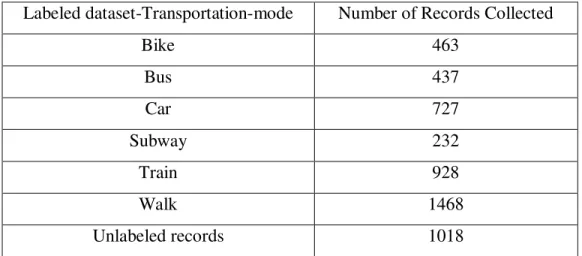
both labeled and unlabeled are shown in Table 3.1:
Table 3.1: Distribution of datasets
3.3. Data Cleaning and preprocessing
Before data is fed into a spatial data mining algorithm, it must be collected, inspected, cleaned
and selected. Since even the best predictor will fail on bad data, data quality and preparation is
crucial. Also, since a predictor can exploit only certain data features, it is important to detect
which data preprocessing works best [28]. For this study preprocessing of the KDD dataset
contains the following processes:
Assigning transportation mode names in to one of the six classes- bike, bus, car, subway, train and walk
To identify and label each transportation mode depending on user documentation of the GeoLife datasets and
Microsoft Excel helps to filter and name easily using fill handle.
There are records which don’t have attributes and these are removed from the dataset. Labeled dataset-Transportation-mode Number of Records Collected
Bike 463
Bus 437
Car 727
Subway 232
Train 928
Walk 1468
26
The Geolife dataset is available in text format; so to be read by the spatial data mining too it has to be changed into CSV (comma separated value) or Attribute-Relation
File Format (ARFF).
3.4. Evaluation Metrics
General performance of spatial data mining systems is measured in terms of numbers of selected features and the classification accuracies of the machine learning algorithms giving the best classification results.
3.4.1. Error Rate
The error rate, which is only an estimate of the true error rate and is expressed to be a good
estimate, if the number of test data is large and representative of the population, is defined as
[46]:
Error Rate= [(Total Test samples- Total Correctly Classified Samples)*100%] /
Total Test Samples ……. 3.3
3.4.2. Accuracy
Overall Classification accuracy (OCA) is the most essential measure of the performance of a
classifier. It determines the proportion of correctly classified examples in relation to the total
number of examples of the test set i.e. the ratio of true positives and true negatives to the total
number of examples. From the confusion matrix, we can say that accuracy is the percentage of
correctly classified instances over the total number of instances in total test dataset, namely the
situation TP and TN, thus accuracy can be defined as follows [47]:
Accuracy = ((TP+TN)*100%)/(TP+TN+FP+FN) …….3.4
3.4.3: Precision and Recall
The parameters are evaluated based on recall accuracy; the definition of precision accuracy and
recall are defined below.
Precision
Precision is defined as the proportion of correctly classified of the specific travel mode (like car,
27
precision is the proportion of true positive to that of the total number of true and false positive
prediction for travel mode A. It is computed as shown in equation 3.5;
---3.5
Predicted Class
Unknown Class
Travel Mode A B
A tp fn
B fp tn
Table 3.2: Exemplifier to compute recall and precision accuracy
Where;
tpA- true positive prediction for class A;
fnA- false negative prediction for class A;
fpA- false positive prediction for class A;
tnA- true negative prediction for class A.
Recall
Recall is defined as the ability of a prediction model to predict instances travel mode correctly
(like walk, car, bus, bike…) Thus, to determine the recall prediction for travel mode A as shown in the Table 3.2, the recall is the proportion of true positive to that of the total number of true
positive and false negative prediction for travel mode A. It is computed as shown in equation 3.6;
---3.6
3.5. Experimentation
This section describes experimental study of the algorithms and procedures, which are described
in the previous chapters. In this research both labeled and unlabeled records are used. Data
mining tool used is Weka and Microsoft Excel used for labeling the datasets and for other
mathematical operations. .
28
The following are the steps used for the experimentation approach:
I. In the beginning, in order to build the experiment, the researcher selected WEKA as the
spatial data mining software used for developing the model; Java command line interface
and DOS interface used for validation the model. Both labeled and unlabeled records were
chosen. All the records considered for this study were taken from five users. All these five
users were navigating in the same region, near Beijing square. At the same time all the
records are consecutives.
II. The selected records are changed from text format into Microsoft excel format. The
Microsoft excel portion of the records contain both labeled and unlabeled records.
III. To come up with cleaned datasets preprocessing tasks are undertaken for underling
missing values, outliers and other issues.
IV. Using the latitude and longitude of every trajectories distance has been calculated from
one point to another point. After calculating the distance between each points, the speed
of travelers from one point to another point can be calculated since time of travelers at
each trajectory point is given.
V. Construct the model using the spatial data mining software packages. The KNN, decision
tree and Navi bayes supervised approach have been selected since the aim of the research
is to classify similar trajectories according to their modes of transportation.
VI. The last step is validating the model using previously unseen records. Speed used as a
major variable for classifying users’ navigation with respect to their transportation mode. The speed is calculated using the distance between consecutive points and the time taken
travel from one point to the next point. Distance is the result of latitude and longitude as
discussed in the beginning of this chapter. And speed is the major variable for the learning
algorithm.
3.5.2. Train the classifier using KNN Algorithm
To train the classifier the researcher applied the classification technique of KNN algorithm. In
the KNN classification algorithm the default value for the k is 1. In the following section, the
researcher has tried to show different results based on the value of K and using speed as
classification criteria. The K value was selected based on the KNN algorithm principle of which
![Figure 2.1: KDD process: “From Knowledge Discovery to Data Mining” [10]](https://thumb-eu.123doks.com/thumbv2/123dok_br/15751679.638122/18.918.168.824.394.601/figure-kdd-process-knowledge-discovery-data-mining.webp)
![Table 2.1: Comparison of DM and KD process models and methodologies [17]](https://thumb-eu.123doks.com/thumbv2/123dok_br/15751679.638122/21.918.138.805.101.546/table-comparison-dm-kd-process-models-methodologies.webp)
![Figure 2.3: Schematic representation of the neural network model [39]](https://thumb-eu.123doks.com/thumbv2/123dok_br/15751679.638122/27.918.231.689.101.395/figure-schematic-representation-neural-network-model.webp)
![Figure 2.4: The structure of Bayes network [19]](https://thumb-eu.123doks.com/thumbv2/123dok_br/15751679.638122/28.918.294.630.110.256/figure-structure-bayes-network.webp)
![Figure 2.5: Simple example of SVM [44]](https://thumb-eu.123doks.com/thumbv2/123dok_br/15751679.638122/29.918.372.600.224.407/figure-simple-example-svm.webp)