Geographic Spatiotemporal Dynamic Model using Cellular
Automata and Data Mining Techniques
Ahmad Zuhdi1, Aniati Murni Arymurthy2 and Heru Suhartanto3
1
Informatics Engineering Dept., Trisakti University and Post Graduate Student in University of Indonesia Jakarta, 11440, Indonesia
2
Faculty of Computer Science, University of Indonesia Depok, 16424, Indonesia
3 Faculty of Computer Science, University of Indonesia
Depok, 16424, Indonesia
Abstract
Geospatial data and information availability has been increasing rapidly and has provided users with knowledge on entities change and movement in a system. Cellular Geography model applies Cellular Automata on Geographic data by defining transition rules to the data grid. This paper presents the techniques for extracting transition rule(s) from time series data grids, using multiple linear regression analysis. Clustering technique is applied to minimize the number of transition rules, which can be offered and chosen to change a new unknown grid. Each centroid of a cluster is associated with a transition rule and a grid of data. The chosen transition rule is associated with grid that has a minimum distance to the new data grid to be simulated. Validation of the model can be provided either quantitatively through an error measurement or qualitatively by visualizing the result of the simulation process. The visualization can also be more informative by adding the error information. Increasing number of cluster may give possibility to improve the simulation accuracy.
Keywords: Geocomputing, Predictive Spatiotemporal Data Mining, Cellular Automata, Continues Transition Rule, Fuzzy c Means Clustering.
1. Introduction
The availability of accumulated geospatial data have been increased exponentially, with a growth rate twice in less than 20 months [14]. This condition is an impact of the tremendous rising of the number of digital transactions and the development of automatic data input techniques, ranging from barcodes, Electronic Data Interchange,
magnetic cards, smartcards, Circuit Camera Television, camera recorders, telephone calls, automatic sensors, remote sensing and so forth. These developments resulted in the size of data stored on a computer system in an organization [18]. They were recorded with remote sensing devices and telescope or an array of micro devices, as well as simulation or recording of data transactions using smart cards, Radio Frequency Identification Data, and Programmable Logic Circuit. On the other hand, the development of studies on the issue and the demand on automatic data analysis become more complex.
However, in contrast to the growth of data volume, the development of analysis techniques for automatic data processing has not show a significant result. The availability of a large data stored in database has invited an intelligent user to dig and find the important knowledge and understanding the phenomena, inference and decision making studies. There is a raising gap, between the availability of data and the analytical knowledge that could be exploited. Therefore, user needs knowledge, which is extracted from the data, using appropriate analysis tool. The study of knowledge extraction technique has been attracted many researchers in various field of study [10].
spatio-temporal trend, which can be presented in sequence of data grids, with dynamic change of their cells. We require modeling of spatiotemporal dynamic, to present relationship between each cell with its surrounding cells. The mechanism changes all of the cell value regularly. The popular approach in this issue is Cellular Geography model, which integrates Geographic Information System approach and Cellular Automata (CA) [13][16].
CA model have been studied on presenting spatial and temporal dynamics of a system [7][4]13]. It has become an interest for researchers to study the model on spatial and temporal dynamic behavior. With CA model, they can explore the complex knowledge of spatiotemporal dynamic by simple computational formulas. Moreover, with adequate thematic and attributes data support and an expert knowledge is needed to formulate an accurate transition rules. This simplicity cause increasing the implementation of CA model, particularly in urban and land use dynamics [1][13][19]. However, in practice it is still difficult to transform the expert knowledge into the transition rule of a CA model, because generally expert knowledge has subjective value and to justify it there is a need the empowerment of spatiotemporal data.
The reliability of data mining engineering, which extract knowledge from large data volume, especially from geographic spatiotemporal, also an interesting study [1][6][ [12][14][16][18]
. The technique is used to extract the dynamics pattern of the spatiotemporal data, especially geographic referenced data, which are expressed in the CA model, by eliciting the CA model transition rules from the existing data sets.
2. Exploration of geographic spatiotemporal
dynamic
Spatiotemporal objects are presented in the form of sequence of 2-d grid consists of mn cells, which is derived from m rows and n columns of a certain spatial data. Their value is updated regularly by following the changes in observation time (called state). It is driven by the transition rules of CA model. These rules determine the dynamics of cell values, which are formulated, based on it cell value and the value of neighboring cells. The main problem in this research is in how to find the transition rules of CA model of spatiotemporal data from geographic data set. The input data was captured from a certain time period of observation, and transition rules are extracted by
applying data mining techniques. Three data mining techniques were applied, namely finding sequential patterns in the data, clustering analysis of the pattern, and classification of a new data grid into certain found of cluster, which had associated with chosen transition rule. We define transition rules elicitation as an exploration of transition rule formula, which is contained in the spatiotemporal data in a grid data set. The formulas can be derived from the change in the cells value of the grid, for subsequent time observation. Hence they are grouped into some clusters, and each cluster has a centroid, which represent a class of transition rule. We can identify the closest transition rule to the centroid and its association grid. The association grid is the first grid used to build the transition rule. We can predict the next state of an observed grid, based on the centroid grid data set, which have association with a class of transition rules. They can be applied to classify an unknown data grid class, because each of data grid which is associate with the cluster, correspond to a transition rule that has been explored. The classification based on distance between data grid, that represent the center of the cluster, and the data grid that will be identified. Chosen transition rule has relation with the closest centroid data grid to the evaluation data grid.
In this study, we propose a research methodology that follows in 7 steps:
i). Applying multiple linear regression analysis to analyze the relationship between cell value at the present with the value of the cell and neighboring cells at the previous time. If the model is built by p pieces of data, then this technique is applied (p-1) times, to produce TR1 , TR2, . . . , TR (p-1), which are candidate of transition rules from data grid in the time series. Transition rule is function of neighborhood cell, it is depended on neighborhood scheme and its radius applied, e.g. equation (1). Two most popular schemes are von Neumann and Moore (see figure 3).
Formulation for transition rule of CA with Moore scheme and R = 1, can be defined as:
C i,j (t+1) = a. C i,j (t) + b.C i-1,j-1 (t) + c.C i-1,j (t) + d. C i-1,j+1 (t) + e.Cij-1 (t) + f.C i,j+1 (t) + g. C i+1,j+1 (t) + h.Ci+1j (t) + k.Ci+1j+1 (t) (1)
Figure 1
General formulation of transition rules for Moore neighborhood scheme with radius R = 1
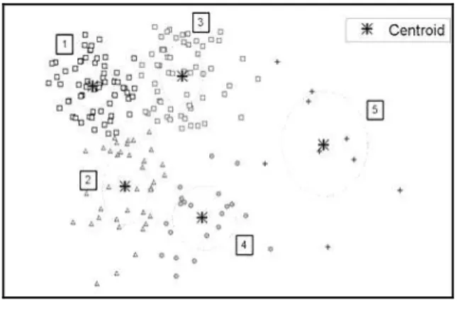
ii. Clustering (p-1) vector TR become the q clusters (q <<p) based on proximity, and visualize it to give users better understanding.
Figure 2
Illustration of Objects Grouping Techniques with Clustering Analysis
iii. Determining the vector representation of the class of patterns (TR), which are relations with the centroids. iv. Determining the closest TR to the centroid, for each cluster and data grid that corresponds with its TR.
v. Utilizing the results of extraction, to classify a new data object, i.e. determining the exact dynamics of the pattern for the new evaluating object.
vi. Testing (calibration) for the model is built, how to measure the validation of models produced.
vii. Evaluating the model, to criticize the advantages and disadvantages of the model.
3. Spatiotemporal Knowledge Exploration
Dynamics of geospatial objects is presented in the form of spatiotemporal trend of geographic data, which requires modeling of spatiotemporal dynamics. The model is visualized in two dimensional grid, which is presented on
mn cells or pixels, each cell has a state variables. Spatial interaction presents the relationship between a cell with its surrounding cells. While the temporal interaction, presents cell value changes at present to the next time. Several techniques had been studied in the exploration of spatiotemporal dynamics knowledge [12], one of which is, knowledge spatiotemporal trends. Prediction of trends is the analysis adopted in data mining, which has reference time. Trend prediction can be explored by applying regression analysis and artificial neural network model. Time series analysis can also provide a fairly accurate approach on knowledge extraction, using sequential patterns to extract the temporal correlation of data.
The application of computational theory to the problems of geography led to discipline of a new study called Geo-computing or geocomputation [11]. It focuses on computer-based modeling and geospatial analysis, and the integration of computational science with the essence of the problems of geographical and terrestrial systems. Geocomputing research grows rapidly, as the growing in collaborative study on computational science and geography, also increasing demand on wide application domain. Geocomputing approach, which is based on the theory and procedures of computation, is effective for problem solving, since it focuses on the simulation of analysis and spatial modeling. Simulation dynamic of geographic object presents spatiotemporal dynamics of physical systems, human systems or both, by examining dynamic processes. The aim is solving or understanding the problem, although they are sometimes contradictory objectives [19]. Building spatiotemporal model, needs three system requirements that must be met, namely the presentation of its spatial, temporal and analytical aspect [8]
. Analytical presentation is related with knowledge structures, stored in the dynamics of the object.
Model CA (S, N, c, t, TR), defined on the grid, which is comprised of m rows and n columns, composed of cells of S. Sij represent one unit area on the earth surface in i-th row j-th column, and has a value (state) cij, deals with the observation variables, can be either qualitative (binary or nominal) or quantitative (numerical, discrete and real). Each cell has neighbor cells, which are determined based on the neighborhood scheme selected.
Figure 3
Popular Neighborhood Scheme
Spatiotemporal dynamic behavior of the grid is defined as the rule of state change or the transition rule. These rules determine the state change of the cell from the present to the next, as presented in equation (2), depending on its state and the neighbor’s state at the present. Transitional rules change the value of cells based on its value and the value of its neighbor’s cells at the previous time [16].
(2) Equation (1) is implementation of formula of equation (2) and Moore neighborhood on figure 3. The defined formula apply a simple form transition rules for R = 1, i.e. outer totalistic approach [3], which was adopted for continues CA. The general form of its formula for R=1 is obtained as follows:
a) If von Neumann's scheme is applied
(3)
b) If Moore’s scheme is applied
(4)
Model of expanded neighborhood scheme, both spatial and spatiotemporal expansion, the number of weight parameters will be extended, for example for the spatial extension of von Neumann's scheme with radius R = 2
then the cells should refer to 9 parameters described in figure 3).
Concept of Data Mining is becoming increasingly popular as an information management tool, since its capability of revealing the structure of knowledge that can lead to decisions under conditions of limited certainty. In many prediction applications, the approach used to understand the data involve logical rules, similarity to evaluate the prototype or through visualization [5]. This techniques can help in classifying and segmenting data and formulating hypotheses.
In this paper, the applied data mining techniques are regression analysis, clustering and classification. Through regression analysis we obtained 29 transition rules that describe the dynamic change from a grid to its subsequence. Clustering technique is applied to select the q ( q << 29 ) alternative transition rules from all the rules, which can be used to predict next state of evaluation grid. Classification Analysis is applied to determine, which the transition rules to be applied to, as described in the research approach.
4. Case Study
Our work studied the dynamic spatiotemporal model of the Fire Danger Rating System (FDRS) based on data of potential drought and smoke or drought code (DC) [9], [17] . Data are downloaded from Indonesia National Outerspace and Aviation Institution, which are published daily. [20]
Figure 4
a sample of Input Data Resource [20]
multiple linear regression analysis on them generates 29 transition rules.
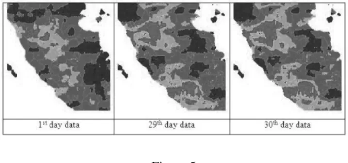
Figure 5
Example of Input Data after pre-processing
Input data are provided in ordinal type y א {0, 1, 2, 3, 4}, each element presents one category of DC, the results of classification based on the real variable x ( 0 < x < 500 ). Spatiotemporal knowledge exploration model is built based on the variable x, so the first problem is the need of transformation that returns the results of classification prior to the computation output in quantitative data. The quantification of qualitative data is conducted in stage 1, namely image segmentation pattern and the transformation of y value into x value. The process observes the dominant RGB value of the five categories of DC, as shown in Table 1. Transformation process of the qualitative data into quantitative values is provided by generating random numbers at each interval associated with each cell value as described in Table 2.
Table 1 Color Segmentation
No .
Color Object Code Characteris-tic
1 White Sea level 0
R > 200 and G > 200 and B > 200
2 Blue
Surface Land / Forest, low DC
1
R <100 and G <100 and B > 200
3 Green
Surface Land /Forest, moderate DC
2
R < 100 and G > 200 and B < 100
Surface R > 200 and
4 Yellow Land / Forest, high DC
3 G > 200 and B < 100
5. Red
Surface Land / Forest, DC extreme
4
R > 200 and G < 100 and B < 100
Table 2 Randomization Data Models
DC Class
Transformation to estimate DC Low Randomize (0, 140) Medium Randomize (141, 260)
High Randomize (261, 350) Extreme Randomize (351,500)
5. Experiments and Result
Our preliminary research shows, that according to random number generator applied, uniform continues distribution is better then normal distribution and uniform discrete distribution. We apply 3 schemes of neighborhood, as shown in figure 3. Application of von Neumann neighborhood with R=2 gives the best result, as we can see in figure 6, so for further experiment we use this scheme.
Figure 6
Performance comparison of 3 neighborhood schemes
5.1 Clustering Analysis
Figure 7
Performance of Fuzzy c Mean clustering Analysis for the transition rules
From figure 7 we can choose number of transition rules, that will be applied for classification an unknown grid. If we use 3 transition rule schemes (figure 3b), then we should identify them, by finding the nearest transition rules to the centroid of the cluster, which associate with them, and also which data grid associate. The experiment result is shown in Table 3:
Table 3
Transition rules number and Grid number, which is associated with centroid
Scheme Centroids (center of
cluster)
Transition Rule# and
Grid# Von
Neumann R=2 and number of cluster
= 3
#1: 0.0002 0.0003 0.0001 0.0002 0.9985 0.0002 0.0002 0.0003 0.0002
#1 is TR 16 associated with 16th grid
#2: 0.0656 0.0875 0.0616 0.0884 0.3523 0.0843 0.0623 0.0843 0.0684
#2 is TR 7 associated with 7th grid
#3: 0.0579 0.0573 0.0560 0.0531 0.4747 0.0529 0.0529 0.0600 0.0631
#3 is TR 6 associated with 6th grid
Figure 7 also shows that an outlier, which is lied near the center of coordinate, can identify a cluster, specifically for itself. The model is used in classification of an unknown data grid, that should be identified, which is the transition rule candidate suitable to apply. Classification process is given in two step, identify the closet data grid associate to the unknown, and choose transition rule number that associated with data grid number to be applied.
5.2 Model Evaluation
Validation model is based on the matching between the two qualitative data, i.e. between testing data and the simulation result data. Simulation process start with running grid#30 for 5 runs, to produce simulation result data Gs1, Gs2, …, Gs5. Output investigation and error calculation based on the comparing between the value of simulation result data and actual data as the testing data The testing data contain of data grid captured after grid#30, i.e. grid # 31 to # 35. Since both are ordinal data type, the difference in value is not applied uniformly, the value should be measured proportionally based on the difference in value of his cell. The largest value = 3, where the maximum difference, the value of simulation data 3 and test data value 0 or vice versa. Value differences 1 (e.g. between extreme and high) are clearly thinner than the 2 (extreme- moderate) and 3 (extreme low). Visualization of the value can be improved understanding of user, with respect to error rate and distribution of the error spatially and temporally.
Errors are calculated based on the percentage deviation between the simulation data and test data, following the formulation as follows:
For example if von Neumann with R=1 applied, U is a matrix with m rows, n columns, from 5 runs simulation process, as simulation results data, and P matrix with the same size as testing data matrix, then the test error model is:
G(U,P).=
1 1 34 0 0 30
{ | ( )ij ij( )|}/(3* * *5)*100%
m n
k l m u t p t m n
In simulation process grid#30 is given as initial state to generate grid#31, grid#32, grid#33, grid#34 and grid#35, the process of classification shows table 4 and figure 7.
Table 4
Simulation result and its error for 3 clusters
No.
Distance Grid-30 to Association Grid Centroids
( 1.0e+004 * )
Nearest Cluster
Grid Ref
Error %
Error Grid
16
Grid7 Grid6
1 3.214 8
3.585 5
3.487 8
1 31 0.177
5 17,7 5
2 3.639 0
3.984 4
3.904 9
1 32 0.209
0 20,9 0
3 3.698 3
4.045 6
3.906 2
1 33 0.225
3 22,5 3
4 3.710 1
4.084 0
3.974 5
1 34 0.241
9 24,1 9
5 3.798 9
4.138 8
4.039 9
1 35 0.257
1
25,7 1
(a) 1st iteration (error 17,75 % )
(b) 2nd Iteration (error 20,90 % )
(c) 3rd Iteration (error 22,53 % )
Figure 8
Simulation result for 3 number of cluster
Finally, our experiment explores error performance, with respect to number of cluster. The comparison is shown in Table 5.
Table 5
Simulation result and its error for (a) 4 clusters and (b) 5 clusters
N o.
Distance Grid-30 to Association
Grid Centroids ( 1.0e+004 * ) Nearest Cluster
Grid Ref
% Error Grid
6 Grid
7 Grid
16
Grid17
1 3.70 10
3.58 77
3.10 98
3.4125 3 31 17,75
2 4.10 51
3.98 16
3.52 15
3.8056 3 32 20,90
3 4.16 46
4.04 71
3.58 55
3.8693 3 33 22,53
34 84 82 5 4.24 78 4.14 74 3.68 72
3.9613 3 35 25,71
(a) N
o.
Distance Grid-30 to Association Grid
Centroids ( 1.0e+004 * ) Near
est Clust
er Grid
Ref %
Err or Grid 17 Grid 24 Grid 4 Grid 7 Grid 16 1 3.12 64 3.11 51 3.44 11 3.41 39 3.10 57
5 31 17,
75 2 3.54 14 3.49 46 3.82 96 3.80 96 3.51 35
2 32 18,
39 3 3.60 60 3.55 08 3.87 65 3.87
00 3.58
67
2 33 18,
82 4 2.98 39 2.96 63 3.21 84 3.22 83 2.94 24
5 34 20,
08 5 3.04 71 3.02 26 3.27 13 3.28 44 3.00 84
5 35 21,
39 (b)
Above figure and table show, there is performance increasing, according to adding the number of cluster from 3 clusters to 4 clusters. The classification result relative stable, since 3 various number of cluster have identical result, that is 5 new data classified to apply transition rule number 16.
Conclusions
In CA based geographic spatiotemporal dynamic model, the magnitude of change is defined by its transition rule. As the dynamic engine, transition rule can be extracted from time series data grids, which are gathered from certain period of time regularly, using multiple linear regression analysis. The quality of transition rules are depends on neighborhood scheme has chosen and its radius R. With the data given in the research, von Neumann neighborhood scheme with R=2 is better then Moore neighborhood and von Neumann neighborhood with R=1.
By clustering technique we can minimize the number of transition rules, which can be offered and chosen to change unknown grid. Each centroid or center of cluster can be associated with a transition rule and a data grid. Transition rule will be applied, is the transition rule which is associate with data grid with minimum distance to the new data grid in simulation. Validation of the model can be provided quantitatively, through error measurement, and qualitatively by visualize the result of simulation process and its error. Visualize error gives more
informative message, because it also show the distribution of error spatially. From experiment result, the increasing number of cluster gives possibility to improve simulation process accuracy.
Actually 30 number of data used in this research is not adequate to get good inference. Its just prototype for building such a simulation tool and explore various system requirement. So, to obtain confidential result of experiment, we have plan to add the number of data at least 100, for building model and testing it. We need to explore more in depth knowledge to improve the performance of the model, which is indicated by its error rate. Some potential improvements according to application of neighborhood scheme, regression analysis scheme and clustering analysis technique.
References
[1] K. Al-Ahmadi, Heppenstall, A. J., Hogg, J. and See, L. M., “A fuzzy cellular automata model of urban growth (FCAUGM) in Riyadh”. Part 2: scenario testing. In review. Applied Spatial Analysis and Policy Journal., 2008
[2] Karl-Heinrich Anders,:How to Visualise Space and Time in "modern" Maps?, Proc. of Joint Workshop Visualization and Exploration of Geospatial Data, vol. XXXVI - 4/W45, Stuttgart, Germany, 2007
[3] Franco Bagnoli, Raúl Rechtman, and Stefano Ruffo, (1992), General algorithm for two-dimensional totalistic cellular automata, Journal of Computational PhysicsVolume 101, Issue 1, July 1992, Pages 176-184
[4] L. Boyer, G. Theyssier, G., “Symposium on Theoretical Aspects of Computer Science 2009” (Freiburg), pp. 195-206,
http://drops.dagstuhl.de/opus/volltexte/2009/1836
[5] Wlodzislaw Duch, Rudy Setiono, Jacek M. Zurada, “Computational Intelligence Methods for Rule-Based Data Understanding”, Proceeding of the IEEE, Vol.92, No.5, May 2004
[6] Mahdi, Esmaeili, Fazekas Gabor, “Finding Sequential Patterns from Large Sequence Data”, IJCSI International Journal of Computer Science Issues, Vol. 7, Issue 1, No. 1, January 2010 ISSN (Online): 1694-0784 ISSN (Print): 1694-0814 43
[8] T. de Senna Carneiro Garcia, “Nested –CA: A Foundation for Multiscale Modeling of Land Use and Land Cover Change”, Doctorate Thesis from the Post Graduation Course in Applied Computer Science, Instituto Nacional de Pesquisas Espaciais (INPE), São José dos Campos, 2007
[9] W J. Groot, , R. D. de · Field, MA. Brady, O. Roswintiarti, M Mohamad” Development of the Indonesian and Malaysian Fire Danger Rating Systems”, Mitig Adapt Strat Glob Change (2006) 12:165–180
[10] R. Grossman, C. Kamath, V. Kumar, “Data Mining for Scientific and Engineering Applications”, Kluwer Academic Publishers, Dordrecht, 2001
[11] Q. Guan, T. Zhang, K.C. Clarke, “GeoComputation in the Grid Computing Age”, W2GIS, Hong Kong, China, 2006
[12] Deren, Li, Shuliang Wang, “Concepts, Principles And Applications Of Spatial Data Mining And Knowledge Discovery”, ISSTM 2005, August, 27-29, 2005, Beijing, China
[13] Ying Long, Shen Zhenjiang, Du Liqun Du, Zhanping Gao Qizhi Mao, “BUDEM: an urban growth simulation model using CA for Beijing metropolitan area” 16th International Conference on GeoInformatics and the Joint Conference on GIS and Built Environment 28-29 June 2008, Guangzhou, China."--P. xix] ISBN 978-0-8194-7385-1
[14] Oded Maimon, Lior Rokach, “Soft Computing for Knowledge Discovery and Data Mining”, Springer Science+Business Media, LLC, 2008
[15] B. Marchionni, D. Ames, H. Dunsford, H. “A Modular Spatial-Temporal Modeling Environment for GIS” 18th World IMACS / MODSIM Congress, Cairns, Australia 13-17 July 2009
[16] Harvey J. Miller, “Geographic Data Mining and Knowledge Discovery”, International Journal of Geographical Information Science, Volume 23, Issue 5 May 2009 , pages 683 - 684
[17] Orbita Roswintiarti, Khomarudin, “Satellite Remote Sensing Based Fire Danger Rating Sys tem to Support Forest/Land Fire Management in Indonesia”, http://www.lapanrs.com/SIMBA
[18] Pang-Ning, Tan, Michael Steinbach, Vipin Kumar, “Introduction to Data Mining”, Addison-Wesley Copyright: 2006
[19] Y. Xie, D. Brown, “Simulation in Spatial Analysis and Modeling”. Computers, Environments and Urban Systems 31(3): 229-231, 2007.
Ahmad Zuhdi, Sarjana in Mathematics (Bandung
Institute of Technology, 1986), MS in Computer Science (University of Indonesia, 1998), Doctor candidate in Computer Science (University of Indonesia), Lecturer and researcher employee at Trisakti University Indonesia.
Aniati Murni Arymurthy, Sarjana in Electrical
Engineering (University of Indonesia), MS in Computer Science (Ohio State University), Doctor of Computer Science (University of Indonesia, 1997), Professor at Faculty of Computer Science University of Indonesia.
Heru Suhartanto, Sarjana in Mathematics (University