Note
A SIMPLIFIED EXCEL
®ALGORITHM FOR ESTIMATING
THE LEAST LIMITING WATER RANGE OF SOILS
Tairone Paiva Leão1; Alvaro Pires da Silva2*
1
University of Tennessee - Dept. of Earth and Planetary Sciences, Graduate Program in Hydrogeology, 1412 Circle Drive 306 - Earth Planetary Sciences Bldg, 37996-1410 - Knoxville, Tennessee, USA.
2
USP/ESALQ Depto. de Solos e Nutrição de Plantas, Av. Pádua Dias, 11, C.P. 9 13418900, Piracicaba, SP Brasil.
*Corresponding author <[email protected]>
ABSTRACT: The least limiting water range (LLWR) of soils has been employed as a methodological approach for evaluation of soil physical quality in different agricultural systems, including forestry, grasslands and major crops. However, the absence of a simplified methodology for the quantification of LLWR has hampered the popularization of its use among researchers and soil managers. Taking this into account this work has the objective of proposing and describing a simplified algorithm developed in Excel® software for quantification of the LLWR, including the calculation of the critical bulk density, at which the LLWR becomes zero. Despite the simplicity of the procedures and numerical techniques of optimization used, the nonlinear regression produced reliable results when compared to those found in the literature.
Key words: nonlinear regression, spreadsheet software, optimization, soil physics, soil quality
UM ALGORITMO SIMPLIFICADO, DESENVOLVIDO EM EXCEL
®,
PARA ESTIMATIVA DO INTERVALO HÍDRICO ÓTIMO DOS SOLOS
RESUMO: O intervalo hídrico ótimo (IHO) dos solos tem sido empregado como uma metodologia para a avaliação da qualidade física do solo em diferentes sistemas agrícolas, incluindo áreas florestais, pastagens e grandes culturas. Entretanto, a inexistência de uma metodologia simplificada para a quantificação do IHO tem dificultado a popularização do uso desta técnica entre pesquisadores e técnicos. Levando isto em consideração, este trabalho tem como objetivo propor e descrever um algoritmo simplificado, desenvolvido em planilha eletrônica Excel®, para quantificação do IHO, incluindo o cálculo da densidade do solo crítica, na qual o IHO é nulo. Apesar da simplicidade dos procedimentos e técnicas numéricas de otimização utilizados, a regressão não-linear produziu resultados confiáveis quando comparados com aqueles encontrados em literatura.
Palavras-chave: regressão não-linear, planilha eletrônica, otimização, física do solo, qualidade do solo
INTRODUCTION
The concept of an index of optimum soil water content for plant growth, as related to soil physical prop-erties was introduced by Letey (1985) and identified as “non-limiting water range” (NLWR). Later, Silva et al. (1994) developed the NLWR concept quantitatively, re-naming it as the least limiting water range (LLWR). For a given soil type, the LLWR incorporates the limitations of soil aeration, matric suction and soil penetration re-sistance for root growth as a function of a single vari-able (i.e. soil bulk density).
Since its quantification (Silva et al., 1994), the LLWR has been employed as an approach for assessing soil physical quality in a wide range of management sys-tems and soils (Tormena et al., 1999; Sharma & Bhusan,
2001; Wu et al., 2003), including in its relation to soil chemical properties (Drury et al., 2003). The LLWR has also been cited as a methodological approach for soil quality assessment in literature reviews (Lal, 2000; Schoenholtz et al., 2000) and books (Brady & Weil, 1999; Silva et al., 2002). Despite advances in the characteriza-tion and quantificacharacteriza-tion of the LLWR, a detailed descrip-tion of the computadescrip-tional methodology for calculating the LLWR from soil properties data, including data manage-ment, curve fitting procedures, and graphing techniques is still lacking.
The objective of this work was to propose a sim-plified algorithm for estimation of the least limiting wa-ter range of soils using the spreadsheet software Microsoft
Excel®1 and discuss technical issues concerning the
non-linear curve fitting procedures. We chose to use Excel®
spreadsheet because it is one of the most popular com-mercial spreadsheets in use in Brazil and many other countries. However, the methodology described here can be adapted to other software packages, according to the resources and knowledge of the user.
THEORETICAL BACKGROUND
The quantification of the Least Limiting Water Range (LLWR) is based on the fitting of a soil water re-tention function and a soil penetration resistance function. The soil water retention function in this specific case must take into account the soil structural variability, which may be achieved by incorporating the soil bulk density in the equation. Silva et al. (1994) incorporated the soil bulk density variability in a simple power function em-ployed by Ross et al. (1991) for fitting the water reten-tion data:
θ = a.Ψ b (1)
θ = Soil volumetric water content [L3 L-3]; Ψ = Matric
suction [M L-1 T-2]; a, b = Empirical parameters.
The stepwise regression procedures of Silva et al. (1994) resulted in a three-parameter nonlinear equation with good fitting properties for characterizing the soil structural influence on the soil water retention phenomena (Tormena et al., 1998; Betz et al., 1998):
θ = exp(a + b.Db). Ψc (2)
θ = Soil volumetric water content [L3 L-3]; D
b = Soil bulk
density [M L-3]; Ψ = Matric suction [M L-1 T-2]; a, b, and
c = Empirical parameters.
The soil penetration resistance function has been adequately described using the nonlinear equation pro-posed by Busscher & Sojka (1987) (Silva et al., 1994; Betz et al., 1998; Leão, 2002).
SR = d.θe.D
b
f (3)
SR = Soil penetration resistance [M L-1 T-2]; θ = Soil
volu-metric water content [L3 L-3]; D
b = Soil bulk density
[M L-3]; d, e, and f = Empirical parameters.
The equations 2 and 3 are transformable to lin-ear form, via logarithmic transformation. Because of the relative simplicity of using linear regression methods, some researchers do prefer to work with them in the lin-earized form (Silva et al., 1994; Betz et al., 1998; Zou et al., 2000). However, we chose not to do so because i) Given the availability of efficient nonlinear algorithms, the usefulness of linearization is somewhat diminished (Seber & Wild, 1989); and ii) The transformation of the data usually involves a transformation of the error term too, which affects the underlying assumptions (Bates & Watts, 1988).
PROPOSED METHODS AND DISCUSSION
The sampling and data collection methodology for the LLWR quantification has been exhaustively de-scribed in other publications (Silva et al., 1994; Leão, 2002; Silva et al., 2002). Briefly, it is necessary to col-lect a set of undisturbed soil cores in the experimental site to be evaluated. The cores are then taken to the labo-ratory and saturated with water. In the lab, each core is equilibrated at different and increased matric suctions (Klute, 1986). The soil penetration resistance, water con-tent and bulk density are then determined in each core. The result is a set of soil penetration resistance (SR),
volumetric water content (θ), bulk density (Db), and
matric suction (Ψ) data points for each one of the cores.
The data is fitted to the Equations 2 and 3, resulting in a set of empirical parameters a, b, c, d, e and f that are used in the quantification of the LLWR.
In the Excel® worksheet example described here,
the first four columns are the data from the silt loam soil described by Silva et al. (1994) (Figure 1). The soil is an
Aquic Eutrochrept with 180 g kg-1 clay, 520 g kg-1 silt, 300
g kg-1 sand and 38 g kg-1 organic matter, and mean bulk
density of 1.47 g cm-3. For the optimization procedures, it
is necessary to create two other columns, with the estimated values for the volumetric water content and soil penetra-tion resistance. This can be achieved by creating columns with Equations 2 and 3, using guess estimates for the em-pirical parameters. It is advisable that the estimates should be taken from the literature, since reasonable initial param-eter estimates are critical for convergence of the optimi-zation algorithms in nonlinear regression (Wraith & Or,
1998). Besides the estimates for the θ and SR equations it
is also necessary to create columns with the squared error (deviate) for these variables (Figure 2). This is necessary for the quantification of the sum of squared error estimates.
The squared error is calculated by:
Error = [(θ or SR)measured – (θ or SR)estimated by the model]2 (4)
With the squared errors for θ and SR, it is
possi-bly to establish cells containing the sum of squared er-rors (SSE) for fitting the Equations 2 and 3. The SSE is the merit function to be minimized in the nonlinear prob-lem optimization in this case. The minimization
proce-dure in Excel® is executed by the command “solver”.
Once the “target cell” is defined, which in this case is the cell containing the sum of squared errors; the option “min” must be selected (Figure 3). The “changing cells” are the parameter estimates previously used to calculate the squared error terms for the variables (Figure 2). It is worth noting that the optimization procedure can be eas-ily subject to constraints. In general, it is not necessary to apply any constraints to fit the equations used in the calculations of the LLWR, as long as good initial param-eter estimates are provided. However, for data sets in which the user suspects low correlation coefficients be-tween the variables it is advisable to apply constraints. The range values for the constraints must be assumed ac-cording to the literature and practicality.
The minimization procedure must be executed independently for variables and parameters of Equations 2 and 3. The goodness of fit can be easily computed from the variance of measured values (a spreadsheet built-in
statistical function) by the coefficient of determination (r2)
of the resulting curve (Figure 4):
r2 = 1 – SSE/N.σ2
variable (5)
N = Number of data points; σ2
variable = Variance of the mea-surements of the independent variable; SSE = Sum of squared errors.
With the parameter estimates, the LLWR for each
Db value can be estimated from simple algebraic
trans-formations of equations 2 and 3. It is also necessary to set the critical limits for the physical variables used in the analysis. Here we used the critical values commonly found in the literature. The field capacity matric suction was set at the value of 0.01 MPa (Haise et al., 1955), and the wilting point was set at 1.5 MPa (Richards & Weaver, 1944). The soil penetration resistance value assumed to be limiting for plant growth was set at 2.0 MPa (Taylor et al., 1966) and the limiting air filled porosity was set at 10% (Grable & Siemer, 1968). However, the user is encouraged to change these critical values according to his experimental conditions and knowledge of the physi-cal processes involved in these critiphysi-cal limits.
The variation in water content at field capacity
(θfc) and wilting point (θwp) with Db can be found by
ap-plying the limiting matric suctions described earlier to Equation 2.
Figure 2 - Columns with estimated values and squared errors for the variables soil penetration resistance and volumetric water content. The parameter estimates for Equations 2 and 3 are shown on the right.
Figure 3 - Optimizer menu for defining target cell, changing cell
θfc = exp(a + b.Db). 0.01c (6)
θwp = exp(a + b.Db). 1.5
c (7)
The variation with Db of the water content at
which the soil penetration resistance is equal to 2.0 MPa
(θsr) can be calculated by isolating the water content in
Equation 3.
θsr = (2.0/ d.Dbf)(1/e). (8)
The variation with Db of the water content at
which the air filled porosity equals 10% (θafp) can be
found from the bulk density and particle density (Dp), here
assumed as 2.65 g cm-3.
θafp = [(1 – Db/Dp)] – 0.1 (9)
The parameters and variables in Equations 6, 7, 8 and 9 are the same as described earlier. The upper limit (UL) of the LLWR can be determined by the lower value
of either θfc or θafp. The lower limit (LL) of the LLWR
can be found by the higher value of either θsr or θwp. The
LLWR is calculated as LLWR = UL – LL and as nega-tive values have no physical meaning in this case, it is necessary to set negative values to zero. This can be
eas-ily achieved in Excel® using the built-in function “IF”.
Figure 5 illustrates the columns with the predicted
values of θfc, θwp, θafp and θsr, along with the results for
the UL, LL and LLWR values calculated using “IF” blocks.
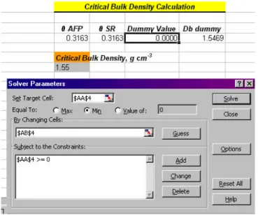
The calculation of soil critical bulk density value
(Dbc) from LLWR is the last and sometimes the most
im-portant step (from soil management point of view) in the
evaluation of the LLWR. To calculate the Dbc it is
neces-sary to know the equations for the variables θfc, θwp, θafp,
and θsr (Equations 6, 7, 8 and 9) and then determine when
UL and LL converge so that the LLWR equals zero. This can be achieved by analyzing which variables in data set defines the first point in which the LLWR equals zero, or by a previous graphic analysis, plotting the variables
θfc, θwp, θafp, and θsr as a function of Db. Once the
equa-tions of the variables that intercept at the point where the
LLWR equals zero are identified, two more cells with these equations need to be established. However, the
equations are drawn as a function of a dummy Db value
that will be optimized to find the Dbc value. Another cell
with a dummy value of the ULequation - LLequation also need
to be created (Figure 6).
At this point, the “solver” command is used again.
The “target cell” will be the dummy value of ULequation
-LLequation. The option “min” is checked and the
“chang-ing cell” will be the cell contain“chang-ing the dummy Db value
(Figure 6). It is necessary to add a constraint pertaining
to the dummy value cell (ULequation - LLequation) that can not
be less than zero in the optimization. After the
optimiza-tion procedure, the Dbc will be equal to the dummy Db,
as shown in Figure 6.
The characteristic LLWR graphics resulting from the procedures described above are illustrated in Figures 7 and 8. Despite the use of simplified statistical proce-dures, similar results were found in comparison to those of Silva et al. (1994). The critical bulk density found by
Excel® Solver (D
bc) was 1.55 g cm
-3, while Silva et al.
(1994) found 1.56 g cm-3. This slight difference in the
val-ues could be attributed to the statistical approaches em-ployed in each case. Silva et al. (1994) used linear re-gression while we choose to use nonlinear rere-gression, for the simplicity of use in this specific case, and to avoid the necessity of linearization of the models, as discussed
earlier. In the Excel® worksheet presented here, Figures
7 and 8 are automatically plotted using the adjusted co-efficients for the models, avoiding the necessity of plot-ting procedures after the statistical analysis. Figure 7
pre-sents the LLWR critical limits by aeration (θafp), field
ca-pacity (θfc), wilting point (θwp) and soil penetration
resis-tance (θsr) plotted as a function of soil bulk density (Db).
An estimate of the dummy Db value and the equations that
Figure 5 - Fixed values of critical limits for field capacity, wilting point, soil penetration resistance, air filled porosity and particle density (left); and estimated values for the least limiting water range (right).
intercept when the LLWR becomes zero are easily visu-alized in Figure 7. This information can be used to fa-cilitate the critical bulk density estimation procedure de-scribed earlier.
Although not estimated in the worksheet
pre-sented here, other relevant Db values for the LLWR
evaluation can be easily quantified using the procedures
described above. These values are: (i) the Db at which
θafp replaces the θfc as the LLWR upper limit, and (ii)
the Db at which θsr replaces θwp as the LLWR lower limit
(Silva & Kay, 1997). Other relevant combinations can be found according to the characteristics of the user’s data.
Another graph that has been widely used in the characterization and interpretation of the LLWR is illus-trated on Figure 8. The variation of the LLWR is
pre-sented as a function of soil Db. From similar graphs,
Tormena et al. (1999) were able to identify important
trends in LLWR data, like ranges of Db values for which
the LLWR is positively correlated, and the Db value at
which LLWR starts to decrease steeply.
CONCLUSIONS
The simplified algorithm presented in this work is an alternative for the time consuming statistical analy-sis and plotting procedures used in the quantification and evaluation of the least limiting water range as an index of soil physical quality. Despite the simplicity of the pro-cedures and numerical techniques of optimization used here, the nonlinear regression produced reliable results when compared to those found in the literature. The criti-cal bulk density value and graphs of LLWR data are also produced by the algorithm, enhancing the interpretation
of the results. The Excel® worksheet is available through
contact with the first author: [email protected].
REFERENCES
BATES, D.M.; WATTS, D.G. Nonlinear regression analysis and its applications. New York: John Wiley & Sons, 1988. 365p.
BETZ, C.L.; ALLMARAS, R.R.; COPELAND, S.M.; RANDALL, G.W. Least limiting water range: traffic and long-term tillage influences in a Webster soil. Soil Science Society of America Journal, v.62, p.1384-1393, 1998.
BRADY, N.C.; WEIL, R.R. The nature and properties of soils. 12.ed. New Jersey: Prentice Hall, 1999. 881p.
BUSSCHER, W.J.; SOJKA, R.E. Enhancement of subsoiling effect on soil strength by conservation tillage. Transactions of the ASAE, v.30, p.888-892, 1987.
DRURY, C.F.; ZHANG, T.Q.; KAY, B.D. The non-limiting and least limiting water ranges for soil nitrogen mineralization. Soil Science Society of America Journal, v.27, p.1388-1404, 2003.
GRABLE, A.R.; SIEMER, E.G. Effects of bulk density, aggregate size, and soil water suction on oxygen diffusion, redox potential and elongation of corn roots. Soil Science Society of America Journal, v.32, p.180-186, 1968.
HAISE, H.R.; HAAS, H.J.; JENSEN, L.R. Soil moisture studies of some Great Plains soils. II. Field capacity as related to 1/3-atmosphere percentage, and minimum point as related to 15- and 26-atmosphere percentage. Soil Science Society of America Proceedings, v.19, p.20-25, 1955.
KLUTE, A. Methods of soil analysis: physical and mineralogical methods. 2.ed. Madison: ASA, 1986. cap.26, p.635-660: Water retention: laboratory methods.
LAL, R. Physical management of soils of the tropics: priorities for the 21st century. Soil Science, v.135, p.191-207, 2000.
LEÃO, T.P. Intervalo hídrico ótimo em diferentes sistemas de pastejo e manejo da pastagem. Piracicaba: USP/ESALQ, 2002. 58p. (Dissertação - Mestrado).
LETEY, J. Relationship between soil physical properties and crop production. Advances in Soil Science, v.1, p.277-294, 1985. RICHARDS, L.A.; WEAVER, L.R. Fifteen atmosphere percentage as related
to the permanent wilting point. Soil Science, v.56, p.331-339, 1944. ROSS, P.J.; WILLIAMS, J.; BRISTOW, K.L. Equations for extending
water-retention curves to dryness. Soil Science Society of America Journal, v.55, p.923-927, 1991.
SCHOENHOLTZ, S.H.; VAN MIEGROET, H.; BURGER, J.A. A review of chemical and physical properties as indicators of forest soil quality: challenges and opportunities. Forest Ecology and Management, v.138, p.335-356, 2000.
LLWR critical limits
0.10 0.20 0.30 0.40 0.50 0.60
1 1.2 1.4 1.6 1.8
Bulk density g cm-3
Volumetric Water Content
cm
3 cm
-3
sr
fc
wp
afp
Figure 7 - Water content variation with bulk density at critical levels of field capacity (fc) at 0.01 MPa, at wilting point (wp) at 1.5 MPa, at air filled porosity (afp) of 10%, and soil penetration resistance (sr) of 2 MPa.
Figure 8 - Variation of the least limiting water range (LLWR) with soil bulk density.
LLWR
0.00 0.05 0.10 0.15
1 1.2 1.4 1.6 1.8
Bulk Density g cm-3
Volumetric Water Content
cm
3 cm
SEBER, G.A.F.; WILD, C.J. Nonlinear regression. New York: John Wiley & Sons, 1989. 768p.
SHARMA, P.K.; BHUSHAN, L. Physical characterization of a soil amended with organic residues in a rice-wheat cropping system using a single value soil physical index. Soil and Tillage Research, v.60, p.143-152, 2001.
SILVA, A.P.; KAY, B.D. Estimating the least limiting water range of soils from properties and management. Soil Science Society of America Journal, v.61, p.877-883, 1997.
SILVA, A.P.; KAY, B.D.; PERFECT, E. Characterization of the least limiting water range of soils. Soil Science Society of America Journal, v.58, p.1775-1781, 1994.
SILVA, A.P.; IMHOFF, S.C.; TORMENA, C.A.; LEÃO, T.P. Avaliação da compactação de solos florestais. In: GONÇALVES, J.L.M.; STAPE, J.L. Conservação e cultivo de solos para plantações florestais. Piracicaba: FEALQ, 2002. cap.10, p.351-372.
TAYLOR, H.M.; ROBERSON, G.M.; PARKER, J.J. Soil strength-root penetration relations to coarse textured materials. Soil Science, v.102, p.18-22, 1966.
TORMENA, C.A.; SILVA, A.P.; LIBARDI, P.L. Caracterização do intervalo hídrico ótimo de um Latossolo Roxo sob plantio direto. Revista Brasileira de Ciência do Solo, v.22, p.573-581, 1998.
TORMENA, C.A.; SILVA, A.P.; LIBARDI, P.L. Soil physical quality of a Brazilian Oxisol under two tillage systems using the least limiting water range approach. Soil and Tillage Research, v.52, p.223-232, 1999. WRAITH, J.M.; OR, D. Nonlinear parameter estimation using spreadsheet
software. Journal of Natural Resources and Life Sciences Education, v.27, p.13-19, 1998.
WU, L.; FENG, G.; LETEY, J.; FERGUSON, L.; MITCHELL, J.; McCULLOUGH-SANDEN, B.; MARKEGARD, G. Soil management effects on the nonlimiting water range. Geoderma, v.114, p.401-414, 2003.
ZOU, C.; SANDS, R.; BUCHAN, G.; HUDSON, I. Least limiting water range: a potential indicator of physical quality of forest soils. Australian Journal of Soil Research, v.38, p.947-958, 2000.(Footnotes)