DEPENDENCE ANALYSIS OF ETHANOL, SUGAR, OIL,
BRL/USD EXCHANGE RATE AND BOVESPA: A VINE
COPULA APPROACH
Anderson Gomes Resende* Osvaldo Candido†
Resumo
Este trabalho tem por objetivo analisar a relação de dependência entre o setor sucroalcooleiro (representado por Etanol e Açúcar), Petróleo, Taxa de Câmbio R$/US$ e o mercado acionário brasileiro (representado pelo ín-dice BOVESPA). A metodologia utilizada é baseada em pair-cópulas e são comparadas três especificações: Regular Vine, a forma mais geral, e dois casos particulares Vine Canônico e Drawable vine. Os resultados obtidos indicaram relações de dependência alinhadas com a literatura existente, mas mostraram que estas relações se alteram significativamente quando a dependência condicional é levada em conta.
Palavras-chave:Commodities; Bio-combustíveis; Dependência multivari-ada; R-Vine cópulas.
Abstract
The aim of this study is to assess the dependence relationship of the sugarcane sector (represented by Ethanol and Sugar), Oil, BRL/USD Ex-change Rate and Brazilian stock market (represented by the BOVESPA – Bolsa de Valores de São Paulo – Index). Our methodology is based on pair-copulas constructions, in which tree specification are compared: Regular Vine, more general, and two particular cases, Canonical vine (C-vine) and Drawable vine (D-vine). Primary results are shown to be aligned with the existing literature but they can change significantly when conditional dependence is taken into account.
Keywords:Commodities; Biofuels; Multivariate dependence; Regular-vine Copulas.
JEL classification:C46, C58, G10.
DOI:http://dx.doi.org/10.1590/1413-8050/ea130174
*Centrais Elétricas do Norte do Brasil S.A. - Eletrobras Eletronorte. E-mail:
†Graduate Program of Economics - Catholic University of Brasilia. E-mail: [email protected]
1
Introduction
In recent years interest regarding renewable fuels has increased around the world, mainly because of their potential of substituting fossil fuels. Some factors have contributed to consolidate these biofuels as a feasible substitute for fossil fuels: the increase of petroleum prices and the debate concerning global warming where the influence of CO2 emissions in this process plays an important role.
The production of biofuels, though still small, has increased steadily due to the adoption by many countries of goals for substituting part of their con-sumption of fossil fuels for renewable ones. The most consolidated initiatives nowadays, ethanol and biodiesel, which are planned to substitute gasoline and diesel oil, respectively, use mostly agro-commodities like corn, wheat, rye, sugar cane, soy and sunflower.
The investigation of how commodity prices interact with fuel prices is of utmost importance, but the conclusions regarding this process are not unani-mous. There are those who advocate that biofuel production generates price distortions in the food market, while others state just the opposite. Mitchell (2008) highlights some difficulties in the comparison of different studies on
that subject. According to him, the estimates can differ widely due to the
dif-ferent periods of time considered, different prices (export/import, wholesale,
retail), and the focus given to different food products. Besides these, the
anal-ysis depends on the currency in which the prices are expressed, and if the in-crease of prices is adjusted by inflation (real) or not (nominal). Another point considered is that different methodologies probably lead to different results.
However, the understanding of how market prices of commodities (agri-cultural, fuel, currencies) related to each other, and how these prices influence and/or are influenced by other asset prices, such as stock market prices is very important for investors when they are setting portfolios and for producers and policy makers, when deciding about production and incentives policies. For example, considering that commodities are drilled, dug, produced and re-fined by companies with public traded stocks, the investors’ decisions in the stock market can affect commodity prices and their availability throughout
the economy. Also, commodity prices and availability can affect stock prices
not only of commodity producing companies, but also of companies in other industries.
Therefore, this paper aims to assess the dependence relationship of the sugarcane market (sugar and ethanol prices), oil prices, the Brazilian Real to the USA Dollar (BRL/USD) exchange rate and the Brazilian Stock Exchange Index (Bolsa de Valores de São Paulo - BOVESPA index).
Several methodologies with different approaches have been used to study
457
variables.
Serra, Zilberman, Gil & Goodwin (2011) model United States daily futures prices of corn, ethanol and oil for the period from July 21, 2005 to May 15, 2007 with a Smooth Transition Vector Error Correction Model (STVECM). The co-integration tests performed support the existence of a (single) long-term relationship between corn, ethanol, and oil prices. Their results also suggest regime changes on that relationship, especially from the strong rise in ethanol prices in mid-2006. From generalized impulse response functions the authors find that a shock in the oil and corn prices, when the system is far from its equilibrium, has an effect on ethanol prices in the same direction.
In addition to the previously mentioned studies, there is a huge amount of literature based on Vector Autoregression and Vector Error Correction (VAR/ VEC) analyzing prices interaction. Zhang et al. (2010) explore biofuel im-pact on global prices of agricultural commodities from a short- and long-term perspective. They use monthly prices for commodities, such as corn, rice, soybeans, sugar, and wheat along with ethanol fuel, gasoline, and oil prices from March 1989 to July 2008. The results indicate no direct relationship between long-term fuel prices and agricultural commodities prices, but con-cerning short term price movements, sugar prices affect all other agricultural
commodities prices, except for rice.
Campos (2010) is another author that investigates the determinants of ethanol and sugar prices in a global context. More specifically, she analyses the impact of international ethanol, sugar, and oil prices on Brazilian (do-mestic) prices and the BRL/USD real exchange rate. It is concluded that the domestic sugar price can be significantly predicted by the international sugar price and by the BRL/USD real exchange rate and that ethanol is influenced by both domestic and international sugar prices.
There is another literature stream that takes into account the presence of conditional hetoroskedasticity in the price series and adds this to VAR/VEC-like models. Serra, Zilberman & Gil (2011), for instance, use the multivariate GARCH (Generalized Autoregressive Conditional Heteroscedasticity) model to investigate changes in price volatility and volatility spillovers in the ethanol industry. An interesting fact is that the authors estimate the co-integration re-lationship for the price series and the multivariate GARCH parameters jointly. They use weekly data series that range from July 2000 to February 2008 for crude oil international prices and Brazilian market prices for sugar and ethanol. The results indicate that oil and ethanol prices are positively related in the long run. Moreover, the empirical analysis suggests that oil prices not only affect the price levels of ethanol, but also their volatility. Thus, the volatility
increase in the oil prices increases ethanol price volatility. Ethanol prices in turn have some impact on sugar prices, which leads to an indirect transmis-sion of oil price volatility to sugar prices.
Zhang et al. (2009), apply the same combination VAR/VEC - Multivariate GARCH model for United States data that comprise weekly series of ethanol, corn, soybean, gasoline, and oil prices for the period from March 1989 to De-cember 2007. Their results indicate that the gasoline prices directly affect
ethanol and oil prices. Furthermore, the results also suggest that there is no long-run relationship among fuel prices (oil, ethanol, and gasoline) and agri-cultural commodities (corn and soybeans). Concerning the ethanol effects on
prices for ethanol, corn and oil for the US market (from 2006 to 2011) and find that oil price volatility does influence ethanol and corn prices in opposition to that found by Zhang et al. (2010). According to the former authors, the effect
of the crude oil price volatility on ethanol and corn price volatility is around 20%, but in periods of great turbulence in the oil market, this effect can reach
50%.
Another approach for the dependence analysis of random variables which has been widely used is the copula-based one. But there are just a few appli-cations of copula-based models to assess the commodities-fuel-exchange rate relationship in the sense we have discussed so far. In Serra & Gil (2012), for instance, an Error Correction copula-GARCH model is used to verify the bio-fuels ability to reduce fuel price fluctuations. The authors model the depen-dence between weekly prices of crude oil, biodiesel, and diesel in Spain from November 2006 to October 2010. The dependence parameters implied by Gaussian and Symmetrized Joe-Clayton (SJC) copulas are obtained for crude oil-biodiesel and crude oil-diesel separately. The results indicate that the de-pendence between crude oil and biodiesel is higher in the lower tail than in the upper tail, suggesting asymmetry to the left, while crude oil-diesel de-pendence tends to be symmetric. The authors conclude that biodiesel pro-tects consumers against crude oil price increases and diesel does not. Similar results are found by Reboredo (2011) and Gregoire et al. (2008), also using copula modeling in the energy market. Nevertheless, these authors use bivari-ate copulas which cannot take into account the conditional dependence of all variables jointly. In this case, one may obtain misleading results.
Considering the discussion so far, the main goal of this work is to assess the dependence structure among sugar, ethanol, and oil prices, the Brazilian Real to USA Dollar (BRL/USD) exchange rate and the Brazilian Stock Exchange In-dex (Bolsa de Valores de São Paulo - BOVESPA inIn-dex) jointly through Regular Vine Copulas.
Joe (1996) originally introduces a method for constructing multivariate distributions based on pair-copulas. Bedford & Cooke (2001, 2002) propose the use of vine diagrams to organize these pair-copula decompositions. The method consists of decomposing a multivariate density in a cascade of bivari-ate copulas and their marginal densities. These Vine Copula models allow us to model the dependence structure among random variables in a more flex-ible and realistic way, since it is possflex-ible to specify joint distributions using copula functions that can be asymmetric and tailored, allowing for a wide range of nonlinear dependence without suffering the curse of dimensionality
problems that arise when modeling data in high-dimensional spaces.
459
2
Pair-copula model
Sklar’s Theorem states that every multivariate cumulative probability distri-bution functionFwith marginalsF1,· · ·, Fn may be written as
F(x1,· · ·, xn) =C(F1(x1), F2(x2),· · ·, Fn(xn)) (1)
In terms of the joint probability density functionf, for an absolutely continu-ousFwith strictly increasing continuous marginsF1,· · ·, Fn, we have
f (x1,· · ·, xn) =c12...n(F1(x1),· · ·, Fn(xn))·f1(x1)· · ·fn(xn) (2)
As highlighted in Aas et al. (2009), the joint probability density functionf
can be factorized as
f (x1,· · ·, xn) =fn(xn)·f (xn−1|xn)·f (xn−2|xn−1, xn)· · ·f (x1|x2,· · ·, xn) (3)
and each marginal conditional density can be written in terms of pair-copulas using
f (x|υ) = c
xυj|υ−j
Fx
υ−j
, Fυj υ−j
·f x υ−j
(4)
for a vectorυwith dimensionn. Hereυ
j is an arbitrarily chosen component
ofυandυ−jcorresponds to the vectorυexcluding this component. It follows that the multivariate density function with dimension ncan be decomposed into its marginal densities and a set of bivariate copulas. The pair-copula de-composition involves marginal conditional distributions of the formF(x|υ). Joe (1996) showed that:
F(x|υ) =
∂ Cx, υj|υ−j
Fx
υ−j
, Fυj υ−j
∂ Fυj υ−j
(5)
2.1 Regular vine copulas
This section presents and summarizes some results and definitions from Diss-mann et al. (2013). An R-vine onnelements is a nested set ofn−1 trees such that the edges of tree j become the nodes of tree j+ 1. The proximity con-dition insures that two nodes in treej+ 1 are only connected by an edge if these nodes share a common node in treej. We notice that the set of nodes in the first tree contains all indexes 1,· · ·, n, while the set of edges is a set of
n−1 pairs of those indexes. In the second tree the set of nodes contains sets of pairs of indexes and the set of edges is built of pairs of indexes, etc.
Formally, an R-vine structure is defined as (Bedford & Cooke 2002)
Definition 1R-Vine Copula Specification(F, V , B)is an R-vine copula
specifi-cation ifF= (F1, . . . , Fn)is a vector of continuous invertible distribution functions,
V is ann-dimensional R-vine andB={Be|i= 1, ..., i−1;e∈Ei}is a set of copulae
withBebeing a bivariate copula, a so-called pair-copula.
A pdf related to the R-vine copula above is given by the product of condi-tional and uncondicondi-tional copulas of each edge.
Theorem 1Let(F, V , B)be an R-vine copula specification on n elements. There
is a unique distributionFthat realizes this R-vine copula specification with density
c(F1(x1),· · ·, Fn(xn)) =
n−1
Y
i=1
Y
e∈Ei
wherexD(e)is the sub-vectorx= (x1,· · ·, xn)indicated by the indexes in the variable D(e).
For C- and D-vines the density (6) can be rewritten in a more convenient way. As in Aas & Berg (2009), and Brechmann & Czado (2013), the canonical vine (C-vine) is a special case of the R-vines class that contains a node with the maximum degree in each tree forming a star structure. In a canonical vine, there aren−1 hierarchical trees with increasing conditional sets and a key variable located at the root of the tree, and there aren(n−1)/2 bivariate copulas.
The drawable vine (D-vine) consists ofn−1 hierarchical trees, with path structures in their sequences and increasing conditional sets, and n(n−1)/2 edges corresponding to each pair-copula.
2.2 Pair-copula model: specification
Dissmann et al. (2013) provides a complete inference procedure for pair-copula decomposition. The procedure consists of the following steps:
a) select an R-vine structure (i.e., unconditional and conditional pairs of variables);
b) select for each pair in a) a bivariate copula family (a pair-copula specifi-cation);
c) estimate all pair-copula parameters.
When modeling low-dimension specifications (e.g. 3 or 4 random vari-ables), it is possible to estimate the parameters of all pairs in the decomposi-tion and compare the resulting log-likelihood. However, in practice, this can become impossible for high-dimension problems.
Thus, following the Dissmann et al. (2013) procedure, in order to choose all pair-copulas and construct the vine structure, one must consider which bi-variate relations are of most importance to model explicitly and let this deter-mine which decomposition is to be used. The main purpose is to concentrate stronger dependences in the first trees, since these dependences are also the most important to model explicitly and precisely. Among the aforementioned three structures , the R-vine and the D-vine are more flexible than the C-vine, because the latter specifies relations between all variables and a key variable and the former one can freely choose which pair to model.
For each pair-copula, the empirical Kendall’s tau (τ) is computed. It does not depend on distributional assumptions, being particularly useful in this case where different combinations of copula families are used. The empirical
Kendall’s tau is given by
τT=PT−QT
T
2
! =
4
T(T−1)PT−1, τ∈[−1,1], (7)
wherePT andQT are the number of concordant and discordant observa-tion pairs respectively.
461
Once the decomposition is chosen, the next step is to specify a parametric copula function, or family, for each pair-copula. The resulting multivariate joint distribution is valid if the copula family that best fits the data is cho-sen for each pair-copula. To choose the most appropriate copula family the Akaike Information Criterion (AIC) is used. The selection procedure consists in assigning an AIC value for each estimated copula function and then select-ing that with the lowest AIC. This process is described in Brechmann & Czado (2013). By using an independence test based on Kendall’s tau, it is possible to specify the product (independence) copula for some pair-copulas. Taking into account that the Kendall’s tau statistic is normal distributed1 with zero mean and variance 2 (2T+ 5)
(9T(T−1)), under the null hypothesis of inde-pendence, independence is rejected with significance of 5% if
s
9T(T−1)
2 (2T+ 5)|τT|>1,96. (8)
Otherwise, if the test indicates independence for any pair-copula, there is no need to evaluate other copula families. One can choose the independence copula in this case.
2.3 Estimation and inference
After adequately choosing all pair-copulas and specifying their respective cop-ula families it is possible to proceed to the estimation of the vine copcop-ula pa-rameters by using the log-likelihood function associated to that. For the an R-vine general specification the log-likelihood is
T X
i=1
n−1
X
l=1
X
e∈El
ln[cj(e),k(e)|D(e)(F(ui,j(e)|ui,D(e)),F(ui,k(e)|D(e)|ui,D(e))|θj(e),k(e)|D(e))]. (9)
Considering the fact that it is common to find tail dependence in financial returns, in addition to the theoretical Kendall’s tau implied by the copula family, the upper, λU , and lower,λL , tail dependence coefficients are also
computed when possible. The population version of Kendall’s tau forX and
Y is given by
τX,Y=P[(X1−X2)(Y1−Y2)>0]−P[(X1−X2)(Y1−Y2)<0]
= 4
Z 1
0
Z 1
0
C(u, v)dC(u, v)−1, (10)
whereCis the copula ofXandY.
Concerning tail dependence coefficients, if a bivariate copula C is such
that limu→11−2u1+−Cu(u, u)=λU exists, thenChas upper tail dependence ifλU∈
(0,1]. Similarly, ifC is such that limu→0C(u, uu ) =λL exists, thenC has lower
tail dependence ifλL∈(0,1].
A tail dependence measure gives us the probability that both variables are located in the upper (or lower) tail of a joint distribution function. With this one can infer simultaneous extreme co-movements.
2.4 Choice among vine-copulas models
In order to make comparisons among R-vine, C-vine and D-vine structures, the Vuong test is applied. Letc1andc2be two vine specifications to be com-pared in terms of their density functions with parametersθ1andθ2. The
stan-dard sum,ν, of the log-difference of punctual probabilities,mi= log
c1(ui|θ1ˆ )
c2(ui|θ2ˆ )
for observationsui∈[0,1], i= 1, ..., T, is given by
v= 1
n PN
i=1mi q
PN
i=1(mi−m¯)2
. (11)
Vuong (1989) shows thatνis asymptotically standard normal distributed. Defining the null hypothesis as H0 :E[mi] = 0∀i = 1, ..., T, the model c1 is chosen instead ofc2 with significanceα ifv >Φ−1
1−α2, whereΦ−1 is the standard normal inverse. Ifv <−Φ−11−α2, the Vuong test is inconclusive. Like the AIC and BIC criteria, the Vuong statistic can be corrected by the number of parameters in the model. There are two possibilities of correction, Akaike and Schwarz which correspond, respectively, to the penalty terms of AIC and BIC. Here the Vuong statistic calculated with no correction, AIC and BIC corrected.
3
Results
3.1 Data
For the empirical application we used weekly time series of the Ethanol anhy-drous (eth) price in USD/Litre and Sugar (sug), USD/50kg price for Crystal sugar, (both from the Center of Advanced Studies on Applied Economics – Luiz Queiroz College of Agriculture/University of São Paulo - CEPEA/ESALQ/USP)2; Oil (oil), Crude oil West Texas Intermediate (WTI) Cushing Oil Spot Price USD/BBL, the Brazilian Real to the US Dollar exchange rate (brus), provided by the Central Bank of Brazil (BCB), and BOVESPA index (bov), index of the Brazilian stock exchange (Bolsa de Valores de São Paulo- BM& F/BOVESPA). The sample size has 639 data points and spans from July 13, 2000 to October 4, 2012.
The inclusion of the variable oil price when performing studies related to the biofuel market is justified, since it is the primary energy input in the world which competes with ethanol and biodiesel. Sugarcane is the main input used in ethanol production in Brazil, so including sugar prices is justified. From the producer point of view sugar can be replaced by ethanol as the final out-put, i.e., producers are able to choose to produce any combination of sugar or ethanol, including only one of them, using sugarcane.
Oil, sugar, and ethanol are internationally traded commodities, so the BRL/USD exchange rate is of great importance for both Brazilian decision makers (producers and government) and investors around the world. And lastly, since financial markets are connected, the Brazilian stock market per-formance can play a role in affecting the aforementioned variables.
2Centro de Estudos de Economia Aplicada – Escola de Agricultura Luiz Queiroz
463
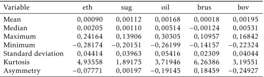
Table 1 shows the summary of statistics of log-returns for the five time series presented above. It can be seen that all series are far from being un-conditionally normal distributed. Except for sugar, all series present positive excess of kurtosis, suggesting that their distributions are leptokurtic, i.e., they are heavy-tailed. The negative excess of kurtosis for sugar indicates its dis-tribution has slender tails. Ethanol, oil, and BOVESPA have a negative asym-metry coefficient, which suggests that negative returns are more frequently
observed than positive ones, while sugar and the BRL/USD exchange rate has a positive asymmetry coefficient.
Table 1: Summary of statistics
Variable eth sug oil brus bov
Mean 0,00090 0,00112 0,00168 0,00018 0,00195
Median 0,00205 0,00110 0,00514 −0,00124 0,00531
Maximum 0,24164 0,13906 0,30305 0,10957 0,16842
Minimum −0,28174 −0,20151 −0,26199 −0,14157 −0,22324
Standard deviation 0,04414 0,03963 0,05416 0,02309 0,04044
Kurtosis 4,93558 1,89175 3,71946 6,26386 3,19551
Asymmetry −0,07771 0,00197 −0,19145 0,18459 −0,24927
The negative asymmetry of oil, ethanol, and BOVESPA can be explained by the 2007/2009 sub-prime crisis period included in our sample, which has adversely impacted those returns. On one hand, oil and ethanol were affected
by the decrease of the world demand and, on the other hand, foreign investors fled Brazil causing a decrease of the BOVESPA index and a depreciation of the Brazilian Real against the US dollar. This can explain the positive asymmetry of the BRL/USD exchange rate log-returns. Conversely, sugar prices have fol-lowed the great increase in agricultural commodity prices in the last years, explaining the greater frequency of positive returns for sugar in the sample.
3.2 Modeling marginal distributions
The marginsF1,· · ·, Fn for the log-returns series in the empirical application
, are modeled using an Autoregressive Moving Average, ARMA (P, d, Q), for the conditional mean, and a Generalized Autoregressive Conditional Het-eroskedasticity, GARCH (p, q), for the conditional variance. The parameter d is included to allow a fractionally integrated process in the conditional mean. Once a model for the marginal distributions is specified, the standardized residuals are taken to be used in the vine copula modeling.
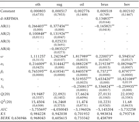
To choose the appropriate order of the parameters P, Q in the mean and p, q in the variance the smallest integer that eliminates the autocorrelation in the standardized residuals and squared standardized residuals is used. In order to test for autocorrelation Ljung-Box Q statistic until lag 20 is used. The results for marginal distributions are presented in Table 2.
Constant-GARCH(1,1)-Table 2: Marginal modeling results
eth sug oil brus bov
Constant 0,000803
(0,6735) 0,(0000517,7853) 0,(0002776,1408) 0,(0000518,749) 0,(0002102,1467)
d-ARFIMA - - - 0,134837∗∗
(0,0164)
-AR(1) 0,266403∗∗∗
(0,000)
0,377456∗∗∗
(0,000)
- −0,165821∗∗
(0,0418)
-AR(2) 0,100848∗∗
(0,0111)
0,131926∗∗∗
(0,0047)
- -
-AR(3) - 0,025231
(0,5691)
- -
-AR(4) - −0,083522∗∗
(0,0273) - -
-ω 1,111257
(0,3115) 1,242364
∗∗
(0,0107) 1,817989
∗∗∗
(0,0023) 0,220073
∗∗
(0,0347) 0,594516
∗
(0,0517) αi 0,216009∗∗
(0,0425)
0,314442∗∗∗
(0,000)
0,088228∗∗∗
(0,0003)
0,219238∗∗∗
(0,0015)
0,082946∗∗∗
(0,0007) βi 0,765395∗∗∗
(0,0000)
0,618541∗∗∗
(0,0000)
0,840578∗∗∗
(0,0000)
0,7572∗∗∗
(0,0000)
0,87977∗∗∗
(0,0000)
νi - - 9,519557∗∗∗
(0,0025)
5,653420∗∗∗
(0,000)
10,821089∗∗
0,0119
λi - - −0,250815∗∗∗
(0,0001) 0,336824
∗∗∗
(0,0017)
−0,259935∗∗∗
(0,000)
Q(20) 19,9487
(0,3357) 22(0,,1402)0921 17(0,,6096)6624 27(0,,1043)0131 22(0,,3383)0392
Q2(20) 15,4504
(0,6308) 16(0,,5753)2468 (011,8731),474 10(0,,9243)2231 (011,8633),68 AIC −3,755697 −4,050045 −3,196026 −5,145204 −3,732258
K S 0,984228 0,942038 0,701932 0,983834 0,793718
BERK0,636946 0,968043 0,605615 0,733342 0,458789 Note:(∗ ∗ ∗), (∗∗), (∗) - significant at 1%, 5%, 10% respectively, p-value between brackets.ω,αandβare theGARCH(1,1) parameters.AIC(Akaike Information criterion).K S(Kolmogorov-Smirnov) andBERK(Berkowitz) are p-value for the uniform distributed test.
Skewed-t for oil, ARFIMA(1,d,0)-GARCH(1,1)-Skewed-t for the BRL/USD ex-change rate and Constant-GARCH(1,1)-Skewed-t for BOVESPA.
By observing the series with standardized residuals Skewed-t distributed, one may see that their conditional distribution is still asymmetric, oil and BOVESPA with negative asymmetry and the BRL/USD exchange rate with positive asymmetry. (Asymmetry was previously indicated by the uncondi-tional statistics in Table 1). Yet, by observing the BRL/USD exchange rate estimates, it can be seen that the parameter for fractional integration, d, is sta-tistically significant. This means that this variable is characterized by a long range dependence process, since , i.e., the BRL/USD exchange rate has long memory.
465
3.3 Modeling the joint distribution through vine copula
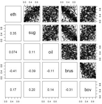
In accordance to the procedure described in section 2.2, it is necessary to in-dicate and select the vine structure, i.e., specify the pair-copula structure so that the strongest pairs-dependence be in the first trees, which can be done using the Kendall’s tau. Figure 1 shows the empirical Kendall’s tau (lower part of the figure) and scatter plots (upper part of the figure) for each pair of transformed margins (PIT of the standardized residuals) modeled in section 3.2.
Figure 1: Kendall’s tau and scatter plots
In order to adequately choose the vine structure for a given data set we have to decide which pair of variables are to be modeled and then specify the respective copula function. The process begins in the first tree that is formed by the pairs which maximize the sum of the absolute values of the Kendall’s tau. Once the first tree is specified, the same is done for the second, the third, and so on until the vine structure specification is completed. After this, the next step is to choose the copula family for each pair-copula and estimate the parameters.
Eight different vine structures in our empirical application are estimated
according to: (i) R-vine, C-vine or D-vine structure; (ii) independence test performed or not, and (iii) family used for the pair-copulas. All models are estimated using VineCopula R package (Schepsmeier et al. 2013). Thus, the estimated models are:
R-vine(with and without the independence test) – each bivariate copula is chosen from elliptical family (Normal and Student-t).
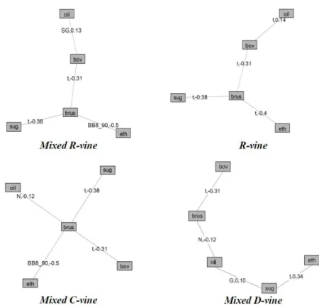
Figure 2 shows the first tree for each estimated model. They are the same with and without the independence test and the families are also the same since in the first tree we always have the strongest bivariate dependences.
Figure 2: First tree of the estimated vine structure
The acronyms on each edge of the trees indicate the copula family used for that specific pair-copula while the number is the Kendall’s tau implied by the respective copula family, e.g., in the Mixed R-vine first tree (upper-left corner of the figure 4) the copula family for the pair sugar-BRL/USD exchange rate (sug-brus) is a Student-t (t) copula with implied Kendall’s tau of -0.38 (The acronyms can be identified by using Table 3).
It is noticeable from the first tree of the R-vine and C-vine specifications that the BRL/USD exchange rate has a main role in these structures, since the other variables have a strong dependence on it, as indicated by the Kendall’s tau. One explanation for this behavior is that the ethanol, sugar, and oil prices are strongly influenced by the import/export dynamics. BOVESPA, in turn, is influenced by the BRL/USD exchange rate through stocks that comprise the index.
ep
en
d
en
ce
an
al
ys
is
of
et
h
an
ol
,
su
ga
r,
oi
l,
B
R
L
/U
SD
ex
ch
an
ge
ra
te
an
d
B
ov
es
p
a
4
6
7
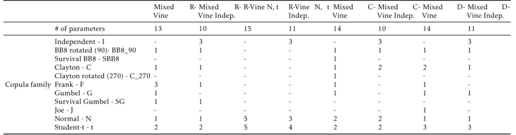
Table 3: Initial description of the vine structures
Mixed
R-Vine
Mixed
R-Vine Indep.
R-Vine N, t R-Vine N, t Indep.
Mixed
C-Vine
Mixed
C-Vine Indep.
Mixed
D-Vine
Mixed
D-Vine Indep.
# of parameters 13 10 15 11 14 10 14 11
Copula family
Independent - I - 3 - 3 - 3 - 3
BB8 rotated (90)- BB8_90 1 1 - - 1 1 1 1
Survival BB8 - SBB8 - - - - 1 - -
-Clayton - C 1 1 - - 1 2 2 1
Clayton rotated (270) - C_270 - - - - 1 - -
-Frank - F 3 1 - - 1 - 1
-Gumbel - G 1 - - - 1 - 1 1
Survival Gumbel - SG 1 1 - - -
-Joe - J - - - 1
-Normal - N 1 1 5 3 2 2 1 1
By using the independence test, ex ante, one can drastically reduce the number of parameters to be estimated when dealing with a large number of variables. Specifically in our case, the greatest reduction occurred in the Mixed C-vine, the model estimated after the independence test has 4 less pa-rameters. The least reduction occurred in the Mixed D-vine and Mixed R-vine, 3 parameters less after the independence test.
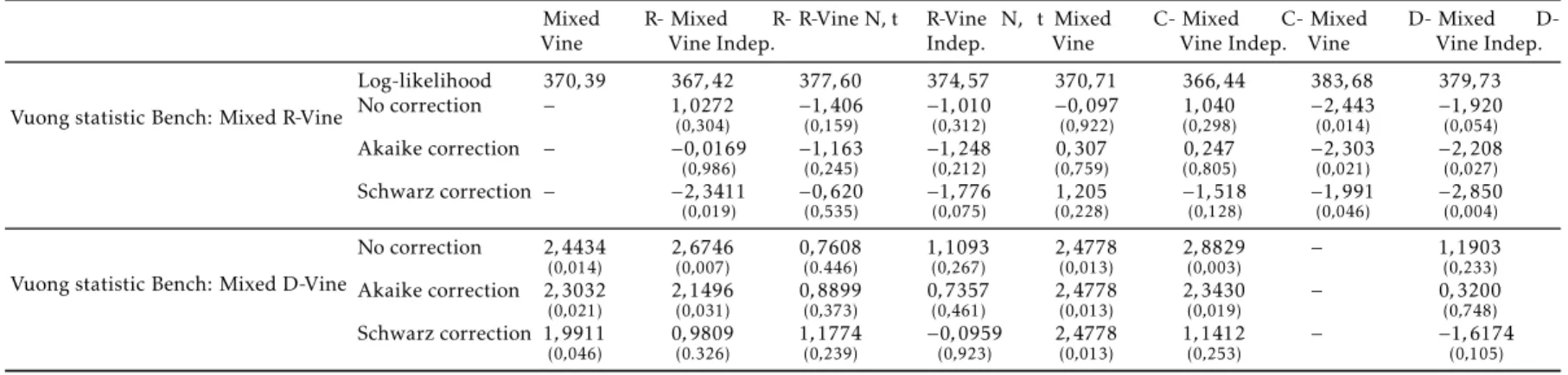
In Table 4 the results for maximum log-likelihood value and the Vuong test for all estimated models are shown. Since the Vuong test is performed in pairs, we have fixed two benchmark models which are compared with all the other ones: Mixed R-vine (more general structure) and Mixed D-vine (the largest log-likelihood value, 383.68). The Voung test is performed considering a significance level 5%.
From Table 4, the Vuong statistics with Akaike correction and no correc-tion, taking Mixed R-vine as the benchmark model and comparing with the Mixed R-vine with independent terms, does not allow the indication of which one is the preferred model. However with Schwarz correction the test indi-cates the Mixed R-vine with independent terms as preferred. This can be explained by the weight assigned to the number of parameters in the Schwarz correction, since the benchmark model has 13 parameters, while the compet-ing one has 7. The Mixed D-vine with and without independent terms are indicated as preferred by the test; the latter by the three statistics and the former by the statistics with Akaike and Schwarz correction. For the other competing models, still taking Mixed R-vine as the benchmark, the Vuong test is inconclusive.
Taking the Mixed D-Vine as the benchmark model, it can be seen that the Mixed D-Vine is indicated as preferred to the Mixed R-vine and Mixed C-vine by all three statistics and also preferred to the Mixed R-C-vine and Mixed C-vine, both with independent terms in accordance to the test with Akaike correction and no correction. For the other competing models the Vuong test is inconclusive.
Therefore, taking into account all the above results, it is possible to infer that the Mixed D-vine is the most indicated model for our dataset since it is indicated by the Vuong test and has the largest log-likelihood value. In spite of this, the results and some comments for all models are presented.
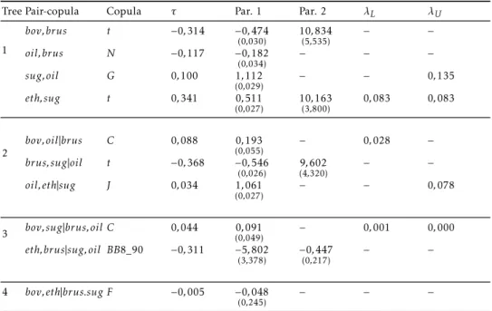
Table 5 presents the estimated parameters for the Mixed D-vine structure. Also shown are the Kendall’s tau, the upper tail dependence (λU) and lower tail dependence (λL), when they exist.
Starting from the first tree of the Mixed D-vine model it can be noticed that there is unconditionally a negative dependence between BOVESPA and the BRL/USD exchange rate (bov,brus). The Kendall’s tau implied by Student-t copula associaStudent-ted Student-to Student-this pair is -0.31. The dependence beStudent-tween oil and Student-the BRL/USD exchange rate is also negative, and the copula for this pair is the Normal one with Kendall’s tau of -0.12, lower than that of BOVESPA and the BRL/USD exchange rate.
The unconditional dependence between ethanol and sugar (eth,sug) is mod-eled by the Student-t copula that reveals a positive dependence, the Kendall’s tau is 0.34, with a symmetrical tail dependence coefficient of 0.08. This
re-sult is compatible with those found in the literature presented previously (see Alves (2002) and Serra, Zilberman & Gil (2011) for instance).
ep en d en ce an al ys is of et h an ol , su ga r, oi l, B R L /U SD ex ch an ge ra te an d B ov es p a 4 6 9
Table 4: Maximum log-likelihood value and Vuong test
Mixed
R-Vine
Mixed
R-Vine Indep.
R-Vine N, t R-Vine N, t Indep. Mixed C-Vine Mixed C-Vine Indep. Mixed D-Vine Mixed D-Vine Indep.
Vuong statistic Bench: Mixed R-Vine
Log-likelihood 370,39 367,42 377,60 374,57 370,71 366,44 383,68 379,73
No correction − 1,0272
(0,304)
−1,406 (0,159)
−1,010 (0,312)
−0,097
(0,922) 1,040(0,298)
−2,443 (0,014)
−1,920 (0,054)
Akaike correction − −0,0169
(0,986)
−1,163 (0,245)
−1,248
(0,212) 0,307(0,759) 0,247(0,805)
−2,303 (0,021)
−2,208 (0,027)
Schwarz correction − −2,3411
(0,019)
−0,620 (0,535)
−1,776 (0,075)
1,205 (0,228)
−1,518 (0,128)
−1,991 (0,046)
−2,850 (0,004)
Vuong statistic Bench: Mixed D-Vine
No correction 2,4434
(0,014) 2,6746(0,007) 0,7608(0.446) 1,1093(0,267) 2,4778(0,013) 2,8829(0,003)
− 1,1903
(0,233) Akaike correction 2,3032
(0,021)
2,1496 (0,031)
0,8899 (0,373)
0,7357 (0,461)
2,4778 (0,013)
2,3430 (0,019)
− 0,3200
(0,748) Schwarz correction 1,9911
(0,046)
0,9809 (0.326)
1,1774 (0,239)
−0,0959 (0,923)
2,4778 (0,013)
1,1412 (0,253)
− −1,6174
(0,105)
Table 5: Estimated parameters for the Mixed D-Vine model
Tree Pair-copula Copula τ Par. 1 Par. 2 λL λU
1
bov,brus t −0,314 −0,474
(0,030) 10(5,,535)834
− −
oil,brus N −0,117 −0,182
(0,034)
− − −
sug,oil G 0,100 1,112
(0,029)
− − 0,135
eth,sug t 0,341 0,511
(0,027)
10,163
(3,800)
0,083 0,083
2
bov,oil|brus C 0,088 0,193
(0,055)
− 0,028 −
brus,sug|oil t −0,368 −0,546
(0,026) 9 ,602
(4,320)
− −
oil,eth|sug J 0,034 1,061
(0,027)
− − 0,078
3 bov,sug|brus,oil C 0,044 (00,,091049) − 0,001 0,000
eth,brus|sug,oil BB8_90 −0,311 −5,802
(3,378)
−0,447
(0,217)
− −
4 bov,eth|brus.sug F −0,005 −0,048
(0,245)
− − −
Note: Standard error between brackets.
Kendall’s tau is 0.1, suggesting a low dependence in the distribution as whole, and the upper tail dependence coefficient is 0.14, which means that sugar and
oil are more dependent in large positive returns (or gains).
In the second tree it is possible to assess conditional dependencies. Let us start with the pair-copula brus,sug|oil, i.e., the dependence between the BRL/USD exchange rate and sugar conditioned on oil. Student-t copula is the family in this case and the Kendall’s tau is -0.37. This means that, conditional on oil, the BRL/USD exchange rate and sugar are highly dependent. This result is as expected since Brazil is a big exporter of sugar and oil has a minor role in relation to the BRL/USD exchange rate and ethanol.
The dependence between BOVESPA and oil conditional on the BRL/USD exchange rate (bov,oil|brus) is characterized by the Clayton copula, asymmet-ric to the left, with overall dependence given by the Kendall’s tau of 0.088 and lower tail dependence coefficient of 0.026, which means that those
vari-ables are conditionally more dependent in large losses, or extreme negative returns. Thus, one can infer that, conditional on the BRL/USD exchange rate, the dependence between BOVESPA and oil is asymmetric to left, though low.
Conversely, conditional on sugar, the dependence relationship between oil and ethanol (oil,eth|sug) is low, the Kendall’s tau is 0.03. But the Joe copula associated to this pair-copula is asymmetric to the right, whose upper tail de-pendence coefficient is 0.08. This can indicate that oil and ethanol conditional
to sugar is more dependent for extreme positive returns.
471
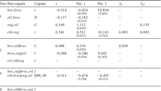
between oil and ethanol, conditional on sugar, the BRL/USD exchange rate (oil,eth|sug,brus) and BOVESPA (oil,eth|bov,brus,sug) is not significant or the independence hypothesis is not rejected (Tables to and Appendix Tables to 13)3.
Table 6: Estimated parameters for the Mixed D-Vine model with independent terms
Tree Pair-copula Copula τ Par. 1 Par. 2 λL λU
1
bov,brus t −0,314 −0,474
(0,030) 10(5,,401)834
− −
oil,brus N −0,117 −0,182
(0,033)
− − −
sug,oil G 0,100 1,112
(0,029)
− − 0,135
eth,sug t 0,341 0,511
(0,027) 10(3,,762)163 0,083 0,083
2
bov,oil|brus C 0,088 0,193
(0,055)
− 0,028 −
brus,sug|oil t −0,368 −0,546
(0,026)
9,602
(4,145)
− −
oil,eth|sug I − − − − −
3 bov,sug|brus,oil I − − − − −
eth,brus|sug,oil BB8_90 −0,311 −5,674
(3,258)
−0,457
(0,212)
− −
4 bov,eth|brus.sug I
Note: Standard error between brackets.
4
Concluding remarks
The main goal of this work is to assess the dependence relationship of the sug-arcane sector, represented by the ethanol and sugar prices, oil prices, Brazil-ian real to US dollar exchange rate and the BrazilBrazil-ian stock market index, rep-resented by the BMF/BOVESPA (Bolsa de Valores de São Paulo) index. To pursue this goal, we used weekly time series of log-returns of the aforemen-tioned prices and index from July 13, 2000 to October 4, 2012, which comprise 639 data points. The methodological procedure is based on pair-copula con-structions and their vine representations. Specifically, Regular vine (R-vine), Canonical vine (C-vine) and Drawable vine (D-vine) structures are estimated, capturing the dependence relationship of all five random variables.
For the marginal distributions, univariate ARMA-GARCH and ARFIMA-GARCH models with Student-t or Skewed-t errors are used. Standardized residuals are obtained from them and then transformed into uniform (0,1) distributed random variables using the probability integral transformation. By the Kolmogorov-Smirnov and Berkowitz tests, it cannot be rejected that the residuals transformed are uniformly distributed on (0,1) interval. Therefore, they can be used to fit the vine copulas model.
Only the Brazilian Real to US Dollar exchange rate has supported a frac-tional integrated process in its condifrac-tional mean equation, indicating the
ence of long range dependence, or long memory. Once the marginal distribu-tions are specified, the Mixed R-vine, D-vine and C-vine structures for the five-dimensional multivariate distribution are fitted, with and without inde-pendent pair-copulas. From the results of the joint distribution modeling it is possible to highlight the following:
- The Brazilian real to US dollar exchange rate has a central role in the de-pendence structure of the multivariate distribution under analysis, i.e., it has a strong negative dependence with the other variables, condition-ally and unconditioncondition-ally.
- Conditional on oil, the Kendall’s tau measuring the dependence between sugar and exchange rate changes from -0.379 to -0.36 and for the ethanol-exchange rate dependence, conditional on sugar and oil, the Kendall’s tau is -0.311.
- Ethanol and sugar have a strong positive dependence, Kendall’s tau of 0.34 and symmetric tail dependence of 0.08.
- Conditional on the Brazilian real to US dollar exchange rate, the pair BOVESPA-oil has a positive relationship (Kendall’s tau is of 0.088 and lower tail dependence of 0.028).
- Oil seems to have low, or no effect on sugar. This may indicate that the
positive relation between oil and sugar, commonly found in the litera-ture, is a result of the exchange rate movement. The same can be said about the oil-ethanol relationship.
- Oil is the variable that has the lowest unconditional dependence with the Brazilian real to US dollar exchange rate, with Kendall’s tau of 0.117.
These results seem to be in line with the Brazilian context. That is, the positive association between ethanol and sugar is related to the capacity of the producers to allocate sugarcane to the production of one to another, even with some technical constraint. Considering the fact that ethanol and sugar are commodities, and the biggest producers are exporters, the strong depen-dence of these variables with the Brazilian real to US dollar exchange rate is explained.
Some pitfalls and further research
473
Some other issues should be taken into account: (1) the time span of the data includes the 2008 Worldwide Financial Crisis. Although the time-varying characteristics of the marginal modeling, i.e., time-time-varying conditional volatilities, capture the impact of the crisis on the individual prices volatilities, the joint dependence parameters do not. This could lead to over- or underes-timated vine-copula parameters. (2) One could question the use of constant copula (dependence) parameters over time (static). Letting parameters evolve over time is a concern for some researchers of Regular Vine Copula modeling. But one must take into account the many issues that arise from making vine copula parameters time-varying, most of them technical issues. First, a time process needs to be specified. Patton (2006) and Silva Filho et al. (2012) model the copula parameters varying through time according to an evolution equa-tion in a bivariate context, which can be extended to a vine context. Second, a two-step IFM estimator may no longer be implemented and only a sequential estimation for the vine parameters can be performed. Those issues imply a greater number of parameters to be estimated and, in general, a less efficient
multi-step estimator will be implemented, which exacerbates the uncertainty concerning the joint estimation of the parameters. To deal with this problem a bootstrap-based estimator for the covariance matrix should be used.
A first direction for further research is to find an appropriate specification for the time evolution of the copula parameters and test whether the depen-dence among ethanol, sugar prices, oil prices, the Brazilian real to US dollar exchange rate, and the Brazilian stock market index is static or dynamic.
A second direction is to increase the number of variables in order to con-sider not only the stock market index but also the stock prices of companies directly related to commodity production, and add substitute commodities for ethanol and sugar.
Those extensions can bring some new empirical insights on the depen-dence among commodities, currencies and stock markets.
Acknowledgments
The authors gratefully acknowledges the financial support of CNPq (406568/ 2012-0 and 453993/2014-1).
Bibliography
Aas, K. & Berg, D. (2009), ‘Models for construction of multivariate depen-dence - a comparison study’,The European Journal of Finance15(7-8), 639– 659.
URL:http://dx.doi.org/10.1080/13518470802588767
Aas, K., Czado, C., Frigessi, A. & Bakken, H. (2009), ‘Pair-copula con-structions of multiple dependence’, Insurance: Mathematics and Economics
44(2), 182 – 198.
URL:http://www.sciencedirect.com/science/article/pii/S0167668707000194
Balcombe, K. & Rapsomanikis, G. (2008), ‘Bayesian estimation and selection of nonlinear vector error correction models: The case of the sugar-ethanol-oil nexus in brazil’,American Journal of Agricultural Economics90(3), 658–668.
URL:http://www.jstor.org/stable/20492320
Bedford, T. & Cooke, R. M. (2001), ‘Probability density decomposition for conditionally dependent random variables modeled by vines’, Annals of
Mathematics and Artificial Intelligence32(1-4), 245–268.
URL:http://dx.doi.org/10.1023/A%3A1016725902970
Bedford, T. & Cooke, R. M. (2002), ‘Vines–a new graphical model for depen-dent random variables’,Ann. Statist.30(4), 1031–1068.
URL:http://dx.doi.org/10.1214/aos/1031689016
Brechmann, E. & Czado, C. (2013), ‘Risk management with high-dimensional vine copulas: An analysis of the euro stoxx 50’,Statistics & Risk
Modeling30(4), 307–342.
Campos, S. K. (2010), Fundamentos econômicos da formação do preço inter-nacional de açúcar e dos preços domésticos de açúcar e etanol, PhD thesis, Escola Superior de Agricultura Luiz de Queiroz, Piracicaba.
Dissmann, J., Brechmann, E., Czado, C. & Kurowicka, D. (2013), ‘Selecting and estimating regular vine copulae and application to financial returns’,
Computational Statistics & Data Analysis59(0), 52 – 69.
URL:http://www.sciencedirect.com/science/article/pii/S0167947312003131
Genest, C. & Favre, A. (2007), ‘Everything you always wanted to know about copula modeling but were afraid to ask’, Journal of Hydrologic Engineering
12(4), 347–368.
URL:http://dx.doi.org/10.1061/(ASCE)1084-0699(2007)12:4(347)
Gregoire, V., Genest, C. & Gendron, M. (2008), ‘Using copulas to model price dependence in energy markets’,Energy Riskpp. 62–68.
Joe, H. (1996), Families of m-variate distributions with given margins
and m(m-1)/2 bivariate dependence parameters, in L. Rueschendorf,
B. Schweizer & M. Taylor, eds, ‘In Distributions with Fixed Marginals and Re-lated Topics’, IMS Lecture Notes-Monograph Series, Hayward, CA., pp. 120– 141.
Mitchell, D. (2008),A Note On Rising Food Prices, The World Bank.
URL:http://elibrary.worldbank.org/doi/abs/10.1596/1813-9450-4682
Patton, A. J. (2006), ‘Modelling asymmetric exchange rate dependence’,
In-ternational Economic Review47(2), 527–556.
URL:http://dx.doi.org/10.1111/j.1468-2354.2006.00387.x
Reboredo, J. C. (2011), ‘How do crude oil prices co-move?: A copula ap-proach’,Energy Economics33(5), 948 – 955.
URL:http://www.sciencedirect.com/science/article/pii/S0140988311000892
475
Serra, T. & Gil, J. M. (2012), ‘Biodiesel as a motor fuel price stabilization mechanism’,Energy Policy50(0), 689 – 698. <ce:title>Special Section: Past and Prospective Energy Transitions - Insights from History</ce:title>.
URL:http://www.sciencedirect.com/science/article/pii/S0301421512006726
Serra, T., Zilberman, D. & Gil, J. M. (2011), ‘Price volatility in ethanol mar-kets’,European Review of Agricultural Economics38(2), 259–280.
URL:http://erae.oxfordjournals.org/content/38/2/259.abstract
Serra, T., Zilberman, D., Gil, J. M. & Goodwin, B. K. (2011), Nonlinearities in the us corn-ethanol-oil price system, 2008 Annual Meeting, July 27-29, 2008, Orlando, Florida 6512, American Agricultural Economics Association (New Name 2008: Agricultural and Applied Economics Association).
URL:http://ideas.repec.org/p/ags/aaea08/6512.html
Silva Filho, O. C., Ziegelmann, F. A. & Dueker, M. J. (2012), ‘Modeling depen-dence dynamics through copulas with regime switching’,Insurance:
Mathe-matics and Economics50(3), 346 – 356.
URL:http://www.sciencedirect.com/science/article/pii/S0167668712000029
Trujillo-Barrera, A., Mallory, M. & Garcia, P. (2011), Volatility spillovers in the u.s. crude oil, corn, and ethanol markets,in‘In: NCCC-134 Conference on Applied Commodity Price Analysis, Forecasting, and Market Risk Man-agement’, St. Louis, Missouri.
Vuong, Q. H. (1989), ‘Likelihood ratio tests for model selection and non-nested hypotheses’,Econometrica57(2), pp. 307–333.
URL:http://www.jstor.org/stable/1912557
Zhang, Z., Lohr, L., Escalante, C. & Wetzstein, M. (2009), ‘Ethanol, corn, and soybean price relations in a volatile vehicle-fuels market’,Energies2(2), 320.
URL:http://www.mdpi.com/1996-1073/2/2/320
Zhang, Z., Lohr, L., Escalante, C. & Wetzstein, M. (2010), ‘Food versus fuel: What do prices tell us?’,Energy Policy38(1), 445 – 451.
URL:http://www.sciencedirect.com/science/article/pii/S0301421509007174
Appendix A
Other estimated models results
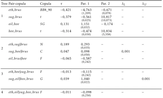
It is worthy to observe the results for the Mixed R-vine in Table A.1 and Mixed C-vine in Table A.2. In the Mixed R-vine the pair-copula oil,bov shows up in the first tree, which corresponds to the unconditional dependence between oil and BOVESPA modeled by the Survival Gumbel copula family with Kendall’s tau and lower tail dependence of 0.13 and 0.17, respectively. This positive relation can be explained by the fact that PETROBRAS (Petroleum Brazil), the 7th biggest energy company in the world, has the greatest participation in the BOVESPA index (8.17% for PTR4 and 2.66% for PTR3 in June 2013), OGX Petroleum has the fourth greatest participation (3.85% for OGXP3), besides some other corporations who depend directly on oil and have participation on the BOVESPA index.
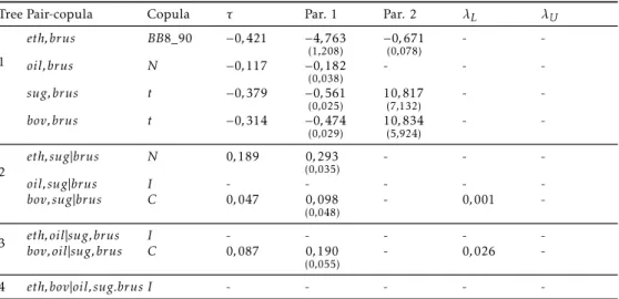
Conditional on sugar and the BRL/USD exchange rate, the dependence be-tween oil and BOVESPA is still positive, Kendall’s tau of 0.098 implied by SBB8 copula (Mixed C-vine) and of 0.087 with lower tail dependence of 0.026 implied by the Clayton copula (Mixed C-vine with independent pair-copulas). Remember that the dependence between BOVESPA and oil conditional on the BRL/USD exchange rate (bov,oil|brus) is characterized by the Clayton copula with Kendall’s tau of 0.088 and lower tail dependence coefficient of 0.026.
Thus, we can conclude that the addition of sugar as a conditioning variable in the pair-copula bov,oil|brus seems to have no impact on the conditional dependence of BOVESPA and oil.
The pair-copula eth,brus has appeared in both Mixed R-vine and Mixed C-vine models (first tree) with Kendall’s tau of -0.42, indicating a strong nega-tive unconditional dependence between ethanol and the BRL/USD exchange rate. The same can be said of the unconditional dependence between sugar and the BRL/USD exchange rate (sug,brus), whose Kendall’s tau is -0.379. Conditional on oil, the dependence between sugar and BRL/USD exchange rate (sug,brus|oil) does not seem to be change significantly. In this case the Kendall’s tau is -0.368.
Considering the dependence between ethanol and sugar conditional on the BRL/USD exchange rate (eth,sug|brus), in the second tree, the Kendall’s tau of 0.19 is noteworthy. The unconditional dependence between these vari-ables is 0.34 (first tree of the Mixed D-vine model – Table 5) and the associated copula is Student-t, with tail dependence coefficient of 0.08. Conditional on
the BRL/USD exchange rate the copula is Normal, with no tail dependence. It is worth noting that both ethanol and sugar are highly related to the BRL/USD exchange rate and highly dependent on each other unconditionally, though, conditional on the BRL/USD exchange rate the dependence between ethanol and sugar is still high.
Conversely, one can compare the unconditional dependence between oil and sugar (sug,oil - first tree of the Mixed D-vine model in Table 5) with that conditional on the BRL/USD exchange rate in the second tree of the Mixed C-vine (oil,sug|brus - Table A.2). For both pair-copulas the related family is the Gumbel copula, but for the conditional case the dependence is less than half of the unconditional one. More precisely, the Kendall’s tau is 0.1 and the upper tail dependence is 0.13 for the unconditional relation and is 0.04 and 0.06 respectively, in the conditional case. Thus, it can be concluded that the dependence between oil and sugar is low and gets even lower when consid-ered conditional on the BRL/USD exchange rate, if in the Mixed C-vine with independent terms (Table A.3), the independence hypothesis is not rejected for the pair-copula oil,sug|brus. When conditional on the BRL/USD exchange rate and BOVESPA, the independence hypothesis is also not rejected for the R-vine with independent terms (Tables and ).
ep
en
d
en
ce
an
al
ys
is
of
et
h
an
ol
,
su
ga
r,
oi
l,
B
R
L
/U
SD
ex
ch
an
ge
ra
te
an
d
B
ov
es
p
a
4
7
7
Table A.1: Estimated parameters for the Mixed R-Vine model
Tree Pair-copula Copula τ Par. 1 Par. 2 λL λU
1
eth,brus BB8_90 −0,421 −4,763
(1,209)
−0,671 (0,078)
− −
sug,brus t −0,379 −0,561
(0,025) 10,817(10,073)
− −
oil,bov SG 0,131 1,151
(0,032)
−0,174 −
bov,brus t −0,314 −0,474
(0,030)
10,834 (5,358)
− −
2
eth,sug|brus N 0,189 0,293
(0,035)
− − −
sug,bov|brus C 0,047 0,098
(0,050)
− 0,001 −
oil,brus|bov F −0,065 −0,587
(0,242)
− − −
3 eth,bov|sug,brus F −0,013 −(00,115,242) − − −
sug,oil|bov,brus G 0,039 1,040
(0,022)
− − 0.001
4 eth,oil|sug,bov,brus F −0,011 −0,098
(0,250)
− − −
Table A.2: Estimated parameters for the Mixed C-Vine model
Tree Pair-copula Copula τ Par. 1 Par. 2 λL λU
1
eth,brus BB8_90 −0,421 −4,763
(1,208)
−0,671
(0,078)
− −
oil,brus N −0,117 −0,182
(0,037)
− − −
sug,brus t −0,379 −0,561
(0,025)
10,817
(8,746)
− −
bov,brus t −0,314 −0,474
(0,029) 10(6,,796)834
− −
2
eth,sug|brus N 0,189 0,293
(0,035)
− − −
oil,sug|brus G 0,042 1,044
(0,024)
− − 0,06
bov,sug|brus C 0,047 0,098
(0,049)
− − −
3 eth,oil|sug,brus F −0,014 −(00,,248)122 − − −
bov,oil|sug,brus SBB8 0,098 1,335
(0,206) 0 ,893
(0,125)
− −
4 eth,bov|oil,sug.brus C_270 −0,010 −0,020
(0,039)
− − −
Note: Standard error between brackets.
Table A.3: Estimated parameters for the Mixed C-Vine model with independent terms
Tree Pair-copula Copula τ Par. 1 Par. 2 λL λU
1
eth,brus BB8_90 −0,421 −4,763
(1,208)
−0,671
(0,078) -
-oil,brus N −0,117 −0,182
(0,038)
- -
-sug,brus t −0,379 −0,561
(0,025)
10,817
(7,132)
-
-bov,brus t −0,314 −0,474
(0,029) 10(5,,924)834 -
-2
eth,sug|brus N 0,189 0,293
(0,035)
- -
-oil,sug|brus I - - - -
-bov,sug|brus C 0,047 0,098
(0,048)
- 0,001
-3 eth,oil|sug,brus I - - - -
-bov,oil|sug,brus C 0,087 0,190
(0,055) - 0,026
-4 eth,bov|oil,sug.brus I - - - -
479
Table A.4: Estimated parameters for the Mixed R-Vine model with independent terms
Tree Pair-copula Copula τ Par. 1 Par. 2 λL λU
1
eth,brus BB8_90 −0,421 −4,763
(1,209)
−0,671
(0,078) -
-sug,brus t −0,379 −0,561
(0,025) 10(9,,033)817 -
-oil,bov SG 0,131 1,151
(0,032) - 0
,174
-bov,brus t −0,314 −0,474
(0,030)
10,834
(5,352)
-
-2
eth,sug|brus N 0,189 0,293
(0,035) - -
-sug,bov|brus C 0,047 0,098
(0,049) - 0,001
-oil,brus|bov F −0,065 −0,587
(0,243)
- -
-3 eth,bov|sug,brus I
sug,oil|bov,brus I
4 eth,oil|sug,bov,brus I
Note: Standard errors between brackets.
Table A.5: Estimated parameters for the Mixed R-Vine Normal/Student-t
Tree Pair-copula Copula τ Par. 1 Par. 2 λL λU
1 eth,brus t −0,399 −(00,027),586 3(0,,943714) 0,008 0,008
sug,brus t −0,379 −0,561
(0,025) 10(4,,375)817 -
-oil,bov t 0,139 0,217
(0,040) 8(3,,626597) 0,033 0,033
bov,brus t −0,314 −0,474
(0,030)
10,834
(5,402)
-
-2 eth,sug|brus N 0,189 0,292
(0,034)
- -
-sug,bov|brus N 0,043 0,068
(0,039) - -
-oil,brus|bov N −0,060 −0,095
(0,039) - -
-3
eth,bov|sug,brus N −0,002 −0,003
(0,039)
- -
-sug,oil|bov,brus t 0,047 0,073
(0,041)
19,714
(13,971)
-
-4 eth,oil|sug,bov,brus N 0,003 0,004
(0,039) - -
Table A.6: Estimated parameters for the Mixed R-Vine Normal/Student-t with inde-pendent
Tree Pair-copula Copula τ Par. 1 Par. 2 λL λU
1 eth,brus t −0,399 −(00,027),586 3(0,,943714) 0,008 0,008
sug,brus t −0,379 −0,561
(0,025) 10 ,817
(4,661) -
-oil,bov t 0,139 0,217
(0,040)
8,626
(3,766)
0,033 0,033
bov,brus t −0,314 −0,474
(0,030)
10,834
(5,418)
-
-2 eth,sug|brus N 0,189 0,292
(0,034) - -
-sug,bov|brus N 0,043 0,068
(0,039) - -
-oil,brus|bov N −0,060 −0,095
(0,039) - -
-3
eth,bov|sug,brus I sug,oil|bov,brus I
4 eth,oil|sug,bov,brus I
Note: Standard error between brackets.
Table A.7: Estimated parameters for the Mixed C-Vine with independent terms
Tree Pair-copula Copula τ Par. 1 Par. 2 λL λU
1 eth,brus BB8_90 −0,421 −(14,,208)763 −(00,,078)671 -
-oil,brus N −0,117 −0,182
(0,038)
- -
-sug,brus t −0,379 −0,561
(0,025)
10,817
(7,132)
-
-bov,brus t −0,314 −0,474
(0,029) 10(5,,924)834 -
-2 eth,sug|brus N 0,189 0,293
(0,035) - -
-oil,sug|brus I - - - -
-bov,sug|brus C 0,047 0,098
(0,048) - 0,001
-3
eth,oil|sug,brus I - - - -
-bov,oil|sug,brus C 0,087 0,190
(0,055) - 0
,026
-4 eth,bov|oil,sug,brus