A Work Project, presented as part of the requirements for the Award of a Masters Degree in Economics from the Nova School of Business and Economics
HEALTH CARE NEEDS AND RESOURCES DISTRIBUTION
How to allocate financial resources in Primary Care Trust?MARTA SOFIA BRANQUINHO DE CAMPOS, 404
A Project carried out on the Economics of Health and Health Care, with the supervision of: Professor Pedro Pita Barros
Abstract
Making a good allocation of the resources available is crucial to ensure a good operation of the system. In Portugal the allocation of resources in Primary Care Trust was made, mainly by historical values.
In the last year, the Central Administration of the Health System proposed a new way of allocating the financial resources in Primary Care Trust.
The goal of this study is to find different possibilities for allocating the financial resources in Primary Care in Portugal. We use data from the Central Administration of the Health System. The Proposal uses linear and quantile regressions, having the per capita costs as a dependent variable. Finally, it was decided on what rule would be better, looking at an economical and statistical criterion.
Introduction
In the health sector, one of the most discussed topics is primary health care. It is considered by many a central pillar of the health system. In order to increase efficiency, quality and equity in this area, countries have increased the complexity of the strategies to provide services in health system. Particularly in Portugal we have seen a lot of changes in the organizations, the largest one having started in 2005. This reform in primary care wants to improve the performance of the health care centres by decentralizing power, increasing team work and giving an active voice to the community. It is within this reform that the Primary Care Trust (namely in Portuguese as Agrupamentos de Centros de Saúde) emerged.
Primary Care Trusts (PCTs) are public health services with administrative and management autonomy consisting of several functional units, constituted by groups of heath care centers. The financing of these groups are made mainly by historical values, which means that they receive the same as the previous year plus a growth rate. The contrato-programa is a contract between the Primary Care Trust and the Regional Health Authority. In this contract the qualitative and quantitative objectives of each Primary Care Trust are settled, together with the resources devoted to compliance and the rules for their implementation.
a different rule to allocate resources, to ensure that primary health resources are being directed where they are most needed.
The goal of this Work Project is to propose a different way of allocating the financial resources in Primary Care Trust in Portugal, given the available data.
The reported is organized in the following way, first, important issues and related literature is explained in section 1. Section 2 will mention a contextualization and an important model to allocate the financial resources proposed by Central Administration of the Health System (ACSS, 2010). Section 3 will make clear the data and the methodology used. Finally, in section 4 and 5 the results will be present, how to implement the formula chosen and the concluding remarks.
1. Literature Review
1.1. Important definitions
The principles of the health service can be stated as equity and efficiency above basic human rights (Carr-Hill and Trevor Sheldon, 1992). The definition of technical efficiency1 is obtaining a determined level of production with the minimum cost (Barros, 2009).
Unlike the meaning of efficiency, the definition of equity is not consensual. In Portugal, equity is defined as equal opportunity of access for those in equal need (Pereira, 1990). Although sometimes this definition is not very clear, in general the decisions of the Portuguese government are in line with this principle.
1
Equity and efficiency are two principles of the health system, but sometimes there are tradeoffs between them, so we need to choose which one will prevail. The selection will depend on the beliefs of the policy makers.
In Portugal, we can say that there are inequities on the distribution of hospital resources (Oliveira and Bevan, 2003). In primary care, there are better results in equity than in quality and there is “a large variation in equity of access to services, in technical efficiency and quality of services across district health authorities” (Amado e Santos, 2009).
The ecological fallacy can occur when we assume that the relationship observed for groups, also necessarily hold for all individuals (Freedman, 1999). To make a capitation formula, ideally we should have individual data, but often studies with aggregate data are the unique option that is available. The advantage of this type of studies is that many times the range of available data is much greater.
The inverse care law stands for “the availability of good medical care tends to vary inversely with the need for the population served. This operates more completely where medical care is most exposed to market forces, and less so where such exposure is reduced." (Hart, 1971). So, it is important that we do not let the market function without any restriction; otherwise it can lead to huge differences in the availability of good medical care.
1.2. Allocate resources by regression in health
On the one hand, there are many countries, like Sweden, England and Belgium that use the risk-adjustment mechanism to reallocate the resources. On the other hand, in Spain there is no risk adjustment, and the same happens in Norway, where the empirical results are determined by political judgment. Even among the countries that use the risk-adjustment mechanism there are many differences in the calculation of the allocation. First, there are differences in the variables, second differences in the statistical tool used and third some countries used data at an individual level (like Sweden), others at an aggregate level (like Belgium) and others both (like England).
In England the formulae to allocate financial resources in health depends on age, at individual level, as well as mortality, morbidity, unemployment, elderly living alone, ethnicity and social status at the aggregate level. The weights given to each variable is decided by experts in health.
The lack of data is a common problem in choosing the variables, so they cannot often do better because they don’t have the data needed. In many countries the choice of the variables is influenced at a greater level by available data than evidence of a link with health needs. Despite this, at an international level there is a lack of investment in new data source (Rice and Smith, 2001).
2.Contextualization
2.1. Portugal
the distribution of resources significantly (Oliveira and Bevan, 2003). The first proposal was thought by the Central Administration of the Health System (ACSS)2.
If we want to create a capitation formula to allocate resources, it is advisable develop a system that provides better data. In a study where the main goal was to develop a capitation formula to measure geographical needs for hospital care in Portugal, the findings were limited by the lack of data (Oliveira and Bevan, 2003).
In the Portuguese health care unit there is no global cost control, since they only manage a small amount of money to cover the cost of operating the health care unit, based on historical costs. The remaining costs3 are paid directly by Regional Health Authority (Barros and Simões, 2007, pp.56).
2.2. Explanation of a model already proposed
Since the goal of this work is to find a formula to allocate the resources in Primary Care Trust and there is already one formula constructed by ACSS (ACSS, 2010), it is important to explain what was proposed. The idea was to construct an index of health needs based on three different components: the health status, the utilization and the determinants of expenditures4. The three quantile regressions calculated for each component are, respectively5:
2 For more details of the model, see section 2.2.
The weights assigned to each component of the index of health needs are calculated by assuming that the health status is the most important so it will weight 50%. Concerning the other two, their weights depend on the R-squared of each component.
Then, the index of health needs and comparing it with the real cost6, was calculated. The first step was to replicate the results of the proposal, which was achieved only partially. There are still some differences, which may be due to rounding.
3. Methodology
3.1. Data
The sample is composed by 68 Primary Care Trusts distributed in 5 different Regional Health Authorities (Norte, Centro, Lisboa e Vale do Tejo, Alentejo e Algarve) and 5 Local Health Units7 (Alto Minho, Baixo Alentejo, Guarda, Matosinhos e Norte Alentejo).
The data was obtained from the Central Administration of the Health System and all information refers to the year 2009, except for the index of purchasing power, which is from 2007.
6 To see more details, see (ACSS, 2010, p. 16).
7 Local Health Unit (LHU) was created to increase the coordination between different levels of care provision,
To begin with, a large improvement would occur by the inclusion of different variables, such as the number of people with chronic diseases, the degree of satisfaction, the quality of the services provided, one variable that represents efficiency, the number of prevention campaigns, among others. However none of these variables were available, so only some new variables were include and improved the model in a different direction.
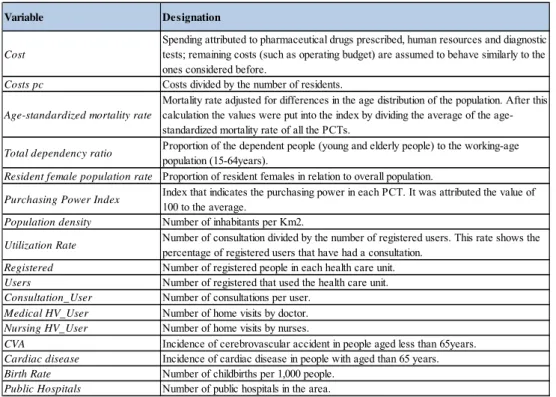
The variables used in this investigation are defined in table 18.
There is no information regarding the number of home visits by nurse per user in 2009 for 3 PCTs (Lisboa V – Odivelas, Algarve II – Barlavento and Pinhal Interior Sul). As a consequence, the value of those PCTs was calculated excluding the missing variable.
3.2.Model
To propose a new rule to allocate resources in the Primary Care Trust, the methodological approach kept the use of a regression, the interest is the analysis of the behaviour of a dependent variable, cost per capita, given the independent variables.
In this study different ways of allocating financial resources in Primary care are proposed. The first way (1)9 represents a small improvement compared what was done by the Central Administration of Health System10. The same variables are used, the only difference concerns the use of the 40th percentile as the quantile reference and the estimation of only one regression instead of three. The regression estimated is as follows:
8
See table 1, page 24.
9The various methods are numbered so that it can be easily understood which model it is being referred to, see
table 2, page 25.
10
It is more accurate to use the 40th percentile instead of the 50th because the 40th percentile takes inefficiencies present in the costs into account: if real cost per capita is used as the dependent variable then, it is very likely that this cost is inefficient, therefore the efficient cost would be lower than the inefficient ones, as a consequence the real cost will push the regression line up.
Another change relates to having all variables being simultaneously used, which means running only one quantile regression, and therefore avoiding weighting indices as stated in the document from ACSS11(ACSS, 2010).
The second way found to allocate financial resources is similar to the previous one, the only difference is the inclusion of more variables.The model (2) is:
0 1 2
3 4
5 6 7 _
8 _ 9 _ 10
11 12 13
In this case, a decision will have to be made regarding which variables to include. As already mentioned the problem to select “good” variables was related to the lack of data. So the choice regarding many of the variables found in the last model, was mainly driven
by the availability of the information, rather than statistical rules. Nevertheless, whenever the introduction of the variable can be justified with being statistically significant, so is done, since that presents some evidence towards the existence of a link between variables used and health needs.
Given the available information, it was decided to include the Standardized mortality rate instead of other similar rates, since the ACSS document (ACSS, 2010) compares different possibilities and reaches the conclusion that this is the best measure because it is the one with the highest R-squared in the per capita cost. Dependency rate and Resident female population were also used because the composition of the population should also be taken into account, since (1) people do not have identical needs for health (Dept. of health and Social Security, 1976) and (2) they are both statistically significant. The Purchasing Power Index and Population density were included because these indexes represent different characteristics of the population served by each PCT. Although these indexes are not statistically significant, it was decided to include them as explanatory variables.
Finally, the incidence of CVA and cardiac disease, birth rate and public hospitals were included because it is thought that they all impact the costs of the health care unit and because they are all statistically significant.
When a regression with all variables is run, it was realized that none of them is statistically significant at a 10% level, so it is crucial to create another model.
The model arose from running a stepwise regression using the variables in the last model. A stepwise regression is a step by step construction of a regression model consisting on eliminating variables based on the statistical significance in the regression. This selection of variables is made through backward selection, which means starting with all candidates and eliminating variables after doing a test. The p-value of an F-statistic is computed for each step, where the null hypothesis is that the coefficient is equal to zero. If it is not possible to reject the null hypothesis, the variable is eliminated. The procedure continues until no further local improvement is possible.
After this procedure is concluded the final model (3) with the surviving variables is: cost pc β β standardized mortality rate β Dependency ratio
β Resident female population β Utilization Rate β Birth Rate u
3.3.Method
Unlike the linear-regression model, in the quantile regression it is possible to estimate different quantile functions of a conditional distribution. Another advantage is that the quantile regression will be more robust in response to large outliers, because it minimizes the absolute distance (Cameron and Trivedi, 2009). It was mainly because of this advantage that this method was chosen instead of the linear-regression model.
To estimate different possibilities of allocate the financial resources we use the quantile regression with the 40% percentile. But sometimes it was not possible to specify it this way12, so we had to use the linear one. Estimates are computed using STATA.
All the methods present in this section are estimated twice, using method 2 and 3. These methods are summarized in the table 213.
To start with, the linear and the quantile regressions of both models were run (2.1/3.1 and 2.2./3.2 respectively).
3.3.1.Separating the PCTs in two groups
There are some Primary Care Trusts (PCTs) that are constrained by supply while others are not, so they face different needs. Given this, it was important to regress them separately. The difficulty of this exercise lies in the definition of an active supply restriction. The only possible way to look at the supply side is the number of users that do not have family doctors assigned to them. Since all the PCTs have users without a family doctor, we cannot divide the sample into PCTs with users with a family doctor versus PCTs with users who do not have family physicians. Therefore another way of dividing the
sample into two has to be determined. One possibility would that of looking at the
evolution of the ratio and check whether there is sudden
change, which could be thought of as the cutoff point of separation of the sample. After analyzing the evolution of the above measure, a considerable change was not found, so this rule was not chosen as the one to be adopted.
First, the bottom 25% PCTs with fewer patients without a family doctor assigned to them was used as the reference, in an ad-hoc way. However, this reference presents a problem: it results in having only a few PCTs in one of the two existing groups. The sample would present the division 18/55 PCTs. Despite this problem, this way of separating the sample in two groups is adopted for the creation of a method (2.3. and 3.3).
Second, the sample was separated, also in an ad-hoc way, in terms of the ratio: users without family doctor divided by total users. In one of the groups PCTs have a ratio higher than 0.1 and in the other PCTs present a ratio smaller than 0.1(methods 2.4. and 3.4.).
Another possible method would be to have the allocation of financial resources included as a normative variable. In this part, normative consultations of the group14 having supply as an active restriction were computed. First, the following linear regression was run for the group that is considered not to be restricted at the supply level (group 1):
In group 1
Variable y represents consultations in model 2 or utilization rate in model 3 (since model 3 does not have consultation as a variable). X’ refers to all the independent variables that represent the characteristics of the population.
is obtained from this linear regression and used in the group 2 (the restricted) to calculate the normative variable. That is:
Then the regression of the restricted group includes the normative variable calculated instead of the normal one. The regression of the unrestricted group is run using the number of consultations realized. The combination of these two regressions allows for the creation of the last methods: 2.5/2.6/3.5/3.6.
3.3.2.Exceptions
As already mentioned, it is better to use the quantile regression, but methods 2.3, 2.4, 2.5 and 2.6 were estimated through linear regressions, because when the quantile regressions of the previously mentioned methods are run, the program used do not mention the value of the t-statistics and the 2-tailed p-values, and the values of each standard error are close to zero.
Another exception can be found regarding methods 2.5 and 2.6, where the inclusion of all variables resulted in having normative variable consultation dropped because of collinearity, in order to overcome this, the regressions15 are computed excluding some of the variables that were used in the estimation of normative consultation (CVA, Cardiac Disease and Birth Rate).
4. Results
After running the regressions and obtaining the results16, it is important to make the decision of which method to apply. Two criteria were constructed to choose the model.
First, one of the possible criteria is from the economic area and is the answer for the question: which variables does it make sense to include in the regression used to allocate financial resources? It is possible to separate the variables into three different groups: the characteristics of the population17, the determinants of health18 and the supply side19. Since (1) the goal is to construct a needs-based allocation formula and (2) there must be a demand for equity in health (and to have equity, an unequal distribution of the resources is needed), it does not make much sense to include several variables of the supply side20. As a consequence, the formula should be more focused on the other two groups of variables rather than in the supply side. Insofar as the goal is to find a formula to allocate the resources in health care centers, the variables should be linked with these centers. The model that is closer to these characteristics is model 321. Within this model, many methods can be chosen.
Second, a statistical criterion was created, which uses the minimum of the sum of absolute residuals, to choose the method.
The hypothesis of using the adjusted R-squared as the index to define the statistical criterion was first considered, but then it was decided not use it: the measure of goodness of
16 See table 4, page 26.
17 In this group are Total dependency ratio, Resident female population rate and Purchasing Power Index. 18 In this group are Age-standardized mortality rate, CVA, Cardiac disease and Birth Rate.
19 In this group are Utilization Rate, Consultation_User, Medical HV_User, Nursing HV_User and Public
Hospitals.
20 Otherwise, it will perpetuate the existent inequities.
21 Model 3 was chosen rather than 1, because 1 has as variable the Purchasing Power Index that is not a
fit of the quantile regression is the pseudo R-squared and, for the sake of statistical accuracy, it could not be compared with the adjusted R-squared of the OLS regressions. Not taking the R-squared of the regressions into account is not worrying, since all regressions that were estimated have sufficiently high R-squared values.
The sum of the absolute residuals is calculated by summing up all the absolute differences between the real and the estimated value, in other words, it is the sum of absolute vertical differences of each point from the regression line.
Although the sum of the absolute residuals is not a goodness of fit criterion, it can be defined as a selection criterion because the goal of this work is to propose a new way to allocate financial resources taking inefficiencies into account.
Considering both criteria is very important and it will result in the choice of the method within the models that meet the economic criteria (model 3) that has the best result according to the statistical criteria.
First, and taking into consideration only the methods with similar procedures to those already proposed by ACSS22 (1, 2.1, 2.2, 3.1 and 3.2), the method chosen after the selection criterion is method 3.1. This method was chosen because it was the one with the lowest sums of absolute residuals among the models selected through the economic criterion. It is important to look deeply at the method chosen23. The analysis of the method chosen provides the expected results: variables Age-standardized mortality rate, Total dependency ratio, Resident female population and Utilization rate have a positive impact on per capita costs. The Birth rate has a negative impact on per capita costs. This can be due to
the existence of a third factor that leads to a high Birth rate and at the same time generates less costs. Users’ age can be thought of as a third factor, since young people are associated to less costs (the elderly are typically the ones causing costs to increase) and more young women should lead to higher birth rates.
Being statistically significant means one can reject the null hypothesis of the coefficient being equal to zero (otherwise the variables would not impact on the cost), hence it is quite important to take this into account. In the method chosen all the variables are statistically significant and the adjusted R-squared is high (0.86).
The Ramsey Regression Equation Specification Error Test (RESET test) is a test that is performed in order to check whether the model presents specification errors. Misspecification can be caused by omitted variables; incorrect functional form or correlation between the independent variables and the error. The null and the alternative hypotheses are:
H0: ui ~ N (0, σ2I)
H1: ui ~ N (µ, σ2I) µ≠0
This means that if specification error is present, the errors will not follow a normal distribution with zero mean.
The results of this test for method 3.1 are positive, which means that we cannot reject the null hypothesis of not having problems.
The presence of homoscedasticity or heteroscedasticity is also important to study. Heteroscedasticity occurs when:
Which means that the variance of the error terms is not constant, causing the Ordinary Least Squares not to produce the Best Linear Unbiased Estimator. The parameter estimates that result from the estimation are not biased; however, the standard errors are.
One way of detecting heteroscedasticity is by calculating the Breusch- Pagan test. In this test the null hypothesis is to have homoscedasticity, i.e., the variance of the error term is constant, versus the alternative hypothesis of not having a constant variance.
Having heteroscedasticity, per si, is not a problem for the progress of this work, given its goals; the problem will arise when using the robust standard deviation, if a wide difference in individual significance of the coefficients is found.
After analyzing the output from the Breusch-Pagan test, we can conclude that in method 3.1 we reject the null hypothesis of having homoscedasticity; however, and since there was not much difference in the significance of the coefficients, it is not a problem to use this method.
Second, taking into account all the methods calculated, the method chosen is 3.324. The method chosen is composed of two regressions, since the PCTs are divided according to the number of people without a family doctor. In the regression of the 25% PCTs with fewest patients without a family doctor, the variables are not statistically significant (only the constant is), but the regression presents a high pseudo R-squared (0.6). The results of the Reset and the B-Pagan tests are good. In the regression of the 75% PCTs with the highest number of patients without a family doctor the statistical results are very different. All variables are statistically significant, the impacts on the cost are the expected
ones and, as always, the pseudo R-squared is high (0.69). But it does not pass in any of the tests.
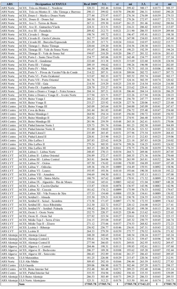
The final allocation provided by method 3.3 is in table 425. The budget needed is less than the real in 2009, which is normal, because in this method, the quantile regression is used, taking cost inefficiencies into account.
4.1.The implementation
After the choice of the method, it is crucial to build an implementation plan. Drastic changes on the budget of each PCT can be catastrophic. So, it is important to smooth the transition process to the new way to allocate financial resources. The partial adjustment model was used for this purpose. In this model the value allocated to each PCT will be a weighted average of the desired and the previous real value, i.e.:
1
is the total expenditure target, Y the total expenditure in the last year, expenditure of each PCT in the last year, the share of each PCT according to the model chosen, (1 is the speed of convergence and is what is transferred to each PCT. With this formula it is guaranteed that the sum of what is transferred is equal to the available budget, i.e.:
X Y was used, which means the total expenditure target is equal to the expenditure in the last year.
The speed of convergence chosen was of 50%, i.e. λ 0.5. Therefore after giving some time for PCTs to adapt to the new budget, this value can increase in the following years. It is thought that the distribution provided by the formula should not cover 100% of the budget because all the variables included in the formula can only explain part of the variation on costs in the PCTs; there are some adjustments to do: the fact that equity should be taken into account and that health statuses are unpredictable provide the rationale for slight deviations from the values predicted by the formula.
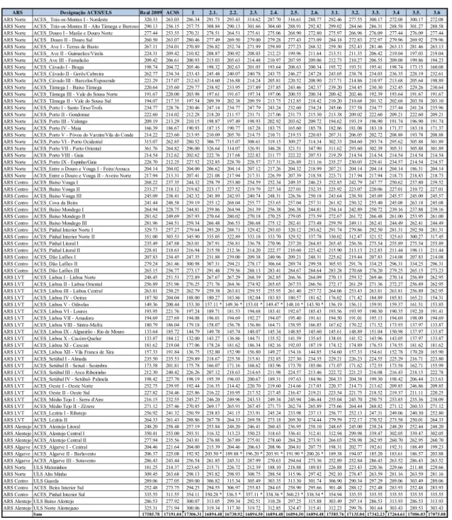
The results obtained according to this way of implementation, and using the models previously chosen, are in table 526.
4.2. Recommendation in the implementation
After carefully choosing which rule we want to implement to redistribute financial resources among Primary Care Trusts, a new phase was started, consisting on the choice the way the formula will in reality be implemented. Choosing the correct way of implementation is just as important as it is to choose the right formula: an excellent rule and a wrong implementation can lead to a complete failure of the new rule.
Humans by nature do not like to change, or at least they find it difficult to adapt to new rules. It’s this statement we should have in mind when planning the implementation of
26
a new rule. First it is very important to be transparent; all the methods, data and procedures should be clearly explained and documented, which means that anyone should be able to replicate the model with the available tools. Secondly, we should use all the resources available, to make sure that everyone understands the new rule. This should all be made before the introduction of the new rule, to prepare people. Thirdly, in case it is possible to do so, one should listen to the constructive criticism in order to include people’s thoughts as part of the process of constructing the formula. This attitude we yield gain receptivity, because people feel the formula is also theirs.
Guaranteeing that this happens, will lead to a more peaceful process and a stable implementation increases the probability of everything going well.
As to technical details, one should make leave others confident that no local budgets will be cut in real terms27, in case it is possible to do so. Given that it can be chaotic to suddenly cut the budget, the guarantee of maintenance of the same level of services provided should be made. Or, at least, not suddenly change from allocation based on historical cost to that based on the formula. This should happen gradually so that people have time to adjust to the new budget.
It is always advisable to look at other examples of adjustments occurring overseas. In one province in Canada, they guarantee that the budget will suffer no cuts in real terms; in Norway there is only a subsidiary role in determining allocation and in other countries, like the Netherlands, provides with some protection to the ones that facing higher variation in terms of the budget received.
27
Following all these steps a plan was constructed to implement the rule that was chosen.
6.Concluding remarks
The purpose of this Work Project was to find possible ways of allocating financial resources among PCTs with the available tools. This work is of the utmost importance since this area has not been duly studied in Portugal and one can foresee an application of a formula reallocating resources in the primary health sector of the Portuguese health system in the near future.
Given that we have significant amounts of money being redistributed, it is recommended to invest in a good system of collecting data. This system should provide viable data and a wider range of available data. It is also highly recommended to follow the steps in the implementation of the formula proposed in this work.
Since, models were built only with the data already available, the range of variables that can be used is reduced. Therefore, it is difficult to choose variables taking into account the incentives faced by providers on the supply of services, the difficulty level of manipulation of information when it is being registered and the persistence of inequalities. Therefore, these aspects were not clearly explored, as they should have. This is left for future research.
What can also be interesting for future research is to analyze the differences in the costs of providing health services depending on the location of PCTs. One possible way of doing this is by controlling for differences in costs between coastal and inland PCTs.
References
Administração Central do Sistema de Saúde. 2010. “ Proposta de alocação normativa de recursos financeiros aos Agrupamentos de Centros de Saúde”. Ministério de Saúde.
Amado, Carla A.E.F. and Sérgio P. Santos. 2009. “Challenges for performance assessment and improvement in primary health care: The case of the Portuguese health centres” Health Policy, 91: 43-56.
Barros, Pedro. 2009. Economia da Saúde conceitos e comportamentos. Coimbra: Edições Almedina.
Barros, Pedro, and Jorde de A. Simões. 2007. “Portugal:Health system review.”Health system in Transition, 9(5): 1-140.
Carr-Hill, Roy, and Trevor Sheldon. 1992. “Rationality and the use of formulae in the allocation of resources to health care.” Journal of Public Health Medicine, 14(2): 117-126.
Department of Health and Social Security. 1976. Sharing Resources for Health in England- Report of the Resource Allocation Working Party. London.
Freedman, David. 1999. “Ecological Inference and the Ecological Fallacy.” University of California Technical Report 549.
Hart, Julian. 1971. “The inverse care law.” The Lancet, 297(7696): 405-412.
Oliveira, Mónica. 2003. “Achieving geographic equity in the Portuguese hospital financing system.” PhD diss. University of London.
Pereira, J. 1990. “Equity objectives in Portuguese health policy.” Social Science and Medicine, 31: 91-94.
Rice, Nigel and Peter C. Smith. 2001. “Capitation and Risk Adjustment in Health Care Financing: An International Progress Report.”, Blackwell Publishers, 79(1): 81-113.
Appendices
Table 1: The designation of the variables used
Medical HV_User
Number of childbirths per 1,000 people. Number of public hospitals in the area.
Incidence of cerebrovascular accident in people aged less than 65years. Number of consultations per user.
Purchasing Power Index
Number of home visits by doctor. Number of home visits by nurses.
Incidence of cardiac disease in people with aged than 65 years.
Utilization Rate
Index that indicates the purchasing power in each PCT. It was attributed the value of 100 to the average.
Number of inhabitants per Km2.
Number of registered people in each health care unit. Number of registered that used the health care unit.
Variable Designation
Total dependency ratio
Population density
Birth Rate
Spending attributed to pharmaceutical drugs prescribed, human resources and diagnostic tests; remaining costs (such as operating budget) are assumed to behave similarly to the ones considered before.
Cost
Mortality rate adjusted for differences in the age distribution of the population. After this calculation the values were put into the index by dividing the average of the age-standardized mortality rate of all the PCTs.
Age-standardized mortality rate
Costs divided by the number of residents.
Costs pc
CVA
Proportion of the dependent people (young and elderly people) to the working-age population (15-64years).
Proportion of resident females in relation to overall population.
Resident female population rate
Number of consultation divided by the number of registered users. This rate shows the percentage of registered users that have had a consultation.
Legend:
a) Represent the regression to the 25% of PCTs with fewer patients without doctor b) Represent the regression to the 75% of PCTs with more patients without doctor
c) Represent the regression to the PCTs with less than 0.1 in the ratio user without doctor divided by users d) Represent the regression to the PCTs with more than 0.1 in the ratio user without doctor divided by users
Table 3: The explanation of all the methods used
De signation Re gre ssion type
1 quantile 2 2.1. linear 2.2. quantile 2.3. linear 2.4. linear 3 3.1. linear 3.2. quantile 3.3. quantile 3.4. quantile
2 regressions, separating PCTs considering the number of people without family doctor. Normative utilization rate used in restricted group
2 regressions, separating PCTs considering the ratio user with no family doctor to total users. Normative utilization rate used in restricted group
2 regressions, separating PCTs considering the number of people without family doctor
Additional comme nts
variables in ACSS document
all variable s available
2 regressions, separating PCTs considering the number of people without family doctor 2 regressions, separating PCTs considering the ratio user with no family doctor to total users 2 regressions, separating PCTs considering the number of people without family doctor. Normative consultations used in restricted group
2 regressions, separating PCTs considering the ratio user with no family doctor to total users. Normative consultations used in restricted group
quantile 3.5. quantile 3.6. linear 2.5. 2.6.
significant variable s only
linear
2 regressions, separating PCTs considering the ratio user with no family doctor to total users Table 2: The regressions of the different models
Cost pe r capita 1. 2.1. 2.2. 2.3. a) 2.3. b) 2.4. c) 2.4. d) 2.5. a) 2.5. b) 2.6. c) 2.6. d) 3.1. 3.2. 3.3 a) 3.3. b) 3.4. c) 3.4. d) 3.5. b) 3.6. d) Standardized Mortality Rate 122.05 133.67 124.72 288.66 136.04 84.35 122.49 185.01 124.28 88.52 103.29 166.46 161.9 70.58 126.61 218.55 121.86 507.59 412.29 (t-statistic) (4.85) (4.26) (1.2) (4.46) (3.86) (1.24) (2.57) (2.47) (3.74) (1.34) (2.27) (6.46) (3.46) (0.24) (4.36) (3.21) (2.28) -0.25 (0.26) Dependency Ratio 2.91 2.07 1.96 6.13 1.78 1.52 2.60 6.91 2.14 2.19 2.77 1.58 1.39 0.59 1.92 0.63 1.94 -7.17 -0.4
(t-statistic) (6.80) (2.35) (0.75) (4.10) (1.91) (0.91) (2.29) (5.15) (2.81) (1.53) (2.22) (3.31) (1.70) (0.14) (3.33) (0.56) (1.76) (-0.13) (-0.02) Resident Population Female 19.23 17.23 24.42 44.03 23.72 16.23 20.05 39.6 33 16.85 27.30 13.77 10.25 -14.71 14.84 8.43 15.76 -28.3 29.39 (t-statistic) (7.36) (3.11) (1.47) (4.68) (3.69) (1.43) (1.98) (3.08) (6.83) (1.58) (3.17) (5.58) (2.50) (-0.52) (5.97) (1.21) (3.48) (-0.10) (0.12) Purchasing Power Parity -0.17 -0.09 -0.26 -3.82 -0.20 -0.31 -0.31 -3.53 -0.58 -0.68 -0.57
(t-statistic) (-1.55) (-0.39) (-0.44) (-5.61) (-0.86) (-0.54) (-0.97) (-4.72) (-4.15) (-1.51) (-2.72) Population Density -4E-04 -0.0008 0.06 -0.003 -0.008 -0.001 0.05 -0.003 -0.01 -0.002 (t-statistic) (-0.13) (-0.14) (4.61) (-1.04) (-0.74) (-0.31) (2.77) (-1.12) (-1.01) (-0.56)
Utilization Rate 3.37 1.38 1.5 2.38 1.25 0.81 1.19 -0.41 1.43 1.2 1.41 2.04 1.98 4.86 1.90 2.56 2.12 (t-statistic) (8.58) (2.45) (0.95) (-1.13) (2.38) (0.63) (1.53) (-01.9) (2.64) (1.04) (2) (4.60) (2.63) (0.70) (3.71) (2.90) (1.99)
Normative Utilization Rate -34.63 23.04
(t-statistic) (-0.14) (0.1)
Consultation_User -5.04 0.21 -32.34 -7.62 -1.82 -1.12 -47.91 -1.14 (t-statistic) (-0.66) (0.01) (-2.15) (-1.03) (-0.11) (-0.11) (-2.56) (-0.07)
Normative Consultation_User 0.32 8.26
(t-statistic) (0.08) (0.33)
Medical HV_User -13.95 8.68 1512.88 116.41 -46.71 805.14 862.60 168.55 17.13 949.3 (t-statistic) (-0.07) (0.01) (2.44) (0.57) (-0.15) (1.53) (1.30) (0.87) (0.06) (2.02) Nursing HV_User 32.28 16.33 185.8 5.66 35.64 34.75 222.62 15.3 36.31 32.6
(t-statistic) (1.05) (0.17) (2.97) (0.18 (0.78) (0.57) (2.62) (0.47) (0.82) (0.60)
CVA 1.1 -1.15 -6.61 1.39 0.21 0.35
(t-statistic) (0.81) (-0.28) (-2.80) (1.06) (0.07) (0.23) Cardiac disease -0.6 0.53 -1.22 -0.58 -0.79 0.29
(t-statistic) (-1.06) (0.26) (-1.03) (-1.04) (-0.81) (0.3)
Birth Rate -10.65 -6 -3.36 -8.75 -9.02 -6.74 -9.97 -7.82 -16.53 -8.83 -7.54 -8.69 -92.84 14.71 (t-statistic) (-2.92) (-0.59) (-0.59) (-2.17) (-1.34) (-1.12) (-4.94) (-2.20) (-0.69) (-3.98) (-1.47) (-1.72) (-0.17) (0.05) Public Hospital -1.6 -1.64 -14.02 -1.16 -2.88 -2.06 -11.68 -1.37 -1.97 -2.07
(t-statistic) (-2.02) (-0.81) (-6.73) (-1.44) (-1.09) (-1.74) (-4.43) (-1.67) (-0.85) (-1.82)
constant 237.07 258.7 247.46 275.42 231.71 258.09 225.71 275.4 232.16 258.10 225.05 240.90 234.73 267.69 227.70 251.24 221.36 223.05 216.09 (t-statistic) (107.10) (15.48) 4.65 (102.01) (68.78) (64.37) (43.73) (74.18) (67.02) (65.68) (47.37) (106.23) (60.62) (14.55) (88.70) (55.73) (44.92) -41.56 -56.21
Number of obs 73 70 70 17 53 36 34 17 53 36 34 73 73 18 55 37 36 55 36
*means that the regression doesnt included the missing variable
ARS Designação ACES/ULS Re al 2009 ACSS 1 2.1. 2.2. 2.3. 2.4. 2.5. 2.6. 3.1. 3.2. 3.3. 3.4 3.5. 3.6
ARS Norte ACES_ Trás-os-Montes I - Nordeste 320.33 263.03 286.34 291.73 293.43 314.62 287.70 316.61 288.77 292.46 277.55 300.17 272.08 300.17 272.08 ARS Norte ACES_ Trás-os-Montes II - Alto Tâmega e Barroso 290.13 256.15 257.75 308.84 290.13 301.66 304.60 288.91 292.82 299.02 284.66 286.31 288.58 301.27 288.58 ARS Norte ACES_Douro I - Marão e Douro Norte 277.44 253.55 270.21 278.51 264.51 275.61 275.06 268.90 272.80 275.97 266.96 276.09 277.44 276.09 277.44 ARS Norte ACES_ Douro II - Douro Sul 260.50 263.07 280.46 277.49 269.50 279.00 279.28 277.43 273.09 284.18 272.83 272.97 279.96 269.92 279.96 ARS Norte ACES_ Ave I - Terras de Basto 267.11 254.01 270.89 256.82 252.74 271.99 259.89 277.23 268.32 259.30 252.43 281.46 263.13 281.46 263.13 ARS Norte ACES_ Ave II - Guimarães/Vizela 224.31 209.42 210.82 208.87 200.92 208.03 212.23 199.96 211.64 213.51 211.35 206.42 219.04 197.03 219.04 ARS Norte ACES_Ave III - Famalicão 209.42 206.61 200.93 215.03 205.63 214.48 210.97 207.95 209.06 212.73 210.27 206.55 209.08 199.86 194.23 ARS Norte ACES_Cávado I - Braga 198.74 204.72 205.46 198.32 202.63 201.05 193.64 208.63 200.34 195.72 193.51 195.41 198.74 173.15 160.08 ARS Norte ACES_Cávado II - Gerês/Cabreira 262.77 234.34 233.43 245.48 240.07 240.78 243.75 246.27 247.28 243.05 238.78 234.03 236.35 228.19 232.61 ARS Norte ACES_Cávado III - Barcelos/Esposende 221.29 217.07 212.63 214.60 216.88 214.24 205.81 220.52 208.90 217.71 214.86 210.97 213.68 205.64 198.89 ARS Norte ACES_Tâmega I - Baixo Tâmega 220.64 235.60 229.77 238.92 233.95 237.89 237.85 243.46 242.37 239.20 234.45 230.30 232.45 229.26 230.64 ARS Norte ACES_Tâmega III - Vale do Sousa Norte 191.67 220.00 203.98 197.61 191.67 197.34 197.06 200.55 200.34 200.42 202.46 192.39 193.64 191.67 191.67 ARS Norte ACES_Tãmega II - Vale do Sousa Sul 194.07 217.35 197.54 209.39 202.38 209.59 213.75 212.85 218.42 210.20 210.68 201.32 202.68 203.58 203.10 ARS Norte ACES_Porto I - Santo Tirso/Trofa 234.77 228.76 230.46 247.14 234.77 247.79 243.24 232.60 234.24 245.06 237.58 234.77 237.44 241.24 235.96 ARS Norte ACES_Porto II - Gondomar 222.60 214.02 212.28 218.20 211.57 231.71 217.06 231.73 215.30 213.38 209.02 222.60 209.21 222.60 209.21 ARS Norte ACES_Porto III - Valongo 209.19 213.29 210.15 198.87 197.49 198.93 202.92 203.62 209.72 194.62 193.19 196.90 191.74 196.90 191.74 ARS Norte ACES_Porto IV - Maia 166.39 186.67 190.93 187.15 190.77 167.28 183.75 165.60 185.78 182.86 181.08 183.18 171.37 183.18 171.37 ARS Norte ACES_Porto V - Póvoa do Varzim/Vila do Conde 214.22 223.60 213.95 210.09 205.70 214.75 210.71 219.53 220.03 207.31 206.05 202.72 208.88 193.78 208.88 ARS Norte ACES_Porto VI - Porto Ocidental 315.07 262.85 280.52 306.77 315.07 308.61 319.15 309.27 314.34 302.33 284.60 293.74 295.62 305.88 301.89 ARS Norte ACES_Porto VII - Porto Oriental 361.76 264.82 296.00 326.64 314.07 326.91 346.28 321.51 347.90 311.62 293.60 302.39 305.31 305.88 301.89 ARS Norte ACES_Porto VIII - Gaia 214.54 212.62 202.62 222.76 217.68 222.82 211.77 222.22 207.53 219.29 214.54 214.54 214.54 214.54 214.54 ARS Norte ACES_Porto IX - Espinho/Gaia 228.70 212.25 227.52 232.85 228.70 228.57 217.31 226.89 211.16 235.27 230.03 229.41 234.57 214.54 234.57 ARS Norte ACES_Entre o Douro e Vouga I - Feira/Arouca 204.14 204.02 204.00 206.62 204.14 207.12 217.26 204.32 218.99 207.21 204.14 204.14 204.14 186.31 204.14 ARS Norte ACES_Entre o Douro e Vouga II - Aveiro Norte 217.94 213.31 207.41 221.08 217.94 217.31 226.59 207.39 218.58 223.71 217.94 217.94 218.73 218.83 218.73 ARS Centro ACES_Baixo Vouga I 268.22 237.35 244.32 258.79 253.80 254.59 252.34 249.35 246.23 252.85 242.79 247.77 250.62 237.80 239.52 ARS Centro ACES_Baixo Vouga II 233.27 218.12 219.82 223.17 227.52 219.79 227.34 227.01 232.35 225.92 223.07 220.06 227.01 210.72 227.01 ARS Centro ACES_Baixo Vouga III 245.09 238.41 242.32 241.89 242.93 240.74 248.31 226.56 250.18 243.64 238.50 245.09 245.57 245.09 245.57 ARS Centro ACES_Cova da Beira 241.44 248.58 239.19 255.12 268.04 255.77 253.65 257.04 257.31 261.82 250.32 255.40 245.08 263.18 245.08 ARS Centro ACES_Baixo Mondego I 264.94 228.75 244.81 259.86 264.94 261.39 256.38 266.38 244.81 254.14 242.89 250.72 239.16 237.88 239.16 ARS Centro ACES_Baixo Mondego II 281.62 249.69 267.93 270.64 280.02 270.18 270.25 279.05 273.59 272.67 261.72 266.48 261.00 253.95 261.00 ARS Centro ACES_Baixo Mondego III 281.96 244.51 259.34 266.48 266.53 286.68 275.12 282.41 273.48 259.59 249.11 262.41 244.49 262.41 244.49 ARS Centro ACES_Pinhal Interior Norte I 329.73 257.27 279.64 293.20 288.71 329.42 293.03 320.12 293.62 291.74 279.86 292.50 281.31 292.50 281.31 ARS Centro ACES_Pinhal Interior Norte II 351.00 303.53 345.90 335.05 322.89 333.18 333.70 329.52 337.78 330.02 312.47 321.52 325.63 300.27 317.45 ARS Centro ACES_Pinhal Litoral I 235.49 247.88 263.01 267.91 256.81 236.78 270.96 237.20 264.85 265.45 256.56 275.54 255.89 275.54 255.89 ARS Centro ACES_Pinhal Litoral II 228.81 218.63 216.94 215.58 212.36 214.20 222.37 210.60 223.42 215.90 213.13 212.83 211.44 198.11 211.44 ARS Centro ACES_Dão Lafões I 207.83 234.45 247.35 231.88 239.00 209.38 240.96 209.21 248.31 225.62 219.44 207.83 214.08 207.83 214.08 ARS Centro ACES_Dão Lafões II 279.24 261.46 300.98 307.31 294.21 278.17 306.64 289.74 299.58 305.93 291.76 334.25 296.31 334.25 296.31 ARS Centro ACES_Dão Lafões III 265.15 256.77 273.17 291.48 279.56 288.13 283.41 284.67 284.64 283.28 270.68 276.20 279.25 265.15 273.23 ARS LVT ACES_Lisboa I - Lisboa Norte 248.45 251.53 272.89 267.67 267.29 268.39 262.85 266.36 264.09 270.13 259.32 269.46 270.14 256.89 262.95 ARS LVT ACES_Lisboa II - Lisboa Oriental 256.89 251.96 276.25 271.76 264.36 274.92 265.65 267.53 266.56 272.17 261.29 271.36 272.27 256.89 262.95 ARS LVT ACES_Lisboa III - Lisboa Central 263.81 250.25 262.79 259.38 263.81 259.55 255.95 261.40 257.72 264.06 253.43 263.81 263.81 256.89 262.95 ARS LVT ACES_Lisboa IV - Oeiras 187.50 204.04 188.00 180.27 183.86 182.04 183.83 180.57 181.62 176.02 171.42 184.89 185.81 165.21 154.31 ARS LVT ACES_Lisboa V - Odivelas 149.36 200.44 153.30 157.11 * 149.36 * 153.01 * 149.47 * 148.10 * 143.50 * 156.19 156.11 159.91 159.37 161.51 153.85 ARS LVT ACES_Lisboa VI - Loures 193.95 221.76 197.24 189.71 181.53 194.68 183.41 192.67 185.43 193.56 193.95 190.30 190.35 192.20 191.41 ARS LVT ACES_Lisboa VII - Amadora 194.69 227.69 194.08 196.01 194.69 192.27 194.07 195.40 191.61 194.50 191.01 195.13 194.69 198.09 194.69 ARS LVT ACES_Lisboa VIII - Sintra-Mafra 180.79 186.04 179.18 158.07 156.78 156.86 164.71 158.95 166.85 167.62 170.22 171.52 173.93 137.97 133.87 ARS LVT ACES_Lisboa IX - Algueirão - Rio de Mouro 133.64 185.72 144.79 149.78 145.74 148.07 145.34 148.85 145.60 145.61 148.89 151.04 150.98 137.97 133.87 ARS LVT ACES_Lisboa X - Cacém-Queluz 133.87 184.12 132.00 143.27 136.86 144.71 135.52 141.59 135.65 138.01 141.52 143.96 143.05 137.97 133.87 ARS LVT ACES_Lisboa XI - Cascais 181.62 219.04 177.06 178.24 181.62 186.34 182.16 192.03 187.19 174.12 174.89 176.53 174.55 181.62 181.62 ARS LVT ACES_Lisboa XII - Vila Franca de Xira 157.33 191.84 136.75 152.80 152.90 156.80 149.27 154.16 144.85 154.60 157.33 154.61 152.78 170.20 165.90 ARS LVT ACES_Setúbal I - Almada 235.50 235.53 229.89 218.67 225.58 215.81 232.85 227.30 234.35 229.21 226.23 224.55 225.29 216.71 223.80 ARS LVT ACES_Setúbal II - Seixal - Sesimbra 173.58 201.81 175.78 166.07 171.16 168.62 183.96 173.70 185.06 171.07 171.62 172.55 173.58 162.71 155.99 ARS LVT ACES_Setúbal III - Arco Ribeirinho 212.30 240.42 226.26 207.12 218.63 214.65 211.98 224.57 213.46 222.72 221.23 216.08 216.43 218.15 222.78 ARS LVT ACES_Setúbal IV - Setúbal- Palmela 198.42 227.70 198.19 195.39 196.03 200.67 189.31 197.63 184.96 204.33 204.38 199.30 198.42 206.44 213.63 ARS LVT ACES_Oeste I - Oeste Norte 252.75 239.95 192.44 216.35 214.42 220.70 219.60 214.66 217.03 220.37 214.73 213.62 209.85 246.86 209.85 ARS LVT ACES_Oeste II - Oeste Sul 227.82 234.46 225.86 216.22 210.95 217.52 217.45 216.47 219.21 223.54 221.75 218.52 219.37 211.11 220.25 ARS LVT ACES_Médio Tejo I - Serra d'Aire 216.15 232.55 245.27 246.20 249.96 243.53 249.34 245.94 246.44 255.04 245.70 250.75 253.85 235.36 238.09 ARS LVT ACES_Médio Tejo II - Zêzere 271.12 257.46 270.85 269.17 265.91 267.45 271.73 262.74 265.89 275.66 264.44 268.82 271.12 260.33 271.12 ARS LVT ACES_Lezíria I - Ribatejo 256.92 241.32 250.59 238.83 241.15 233.91 245.24 233.98 237.13 256.77 252.13 247.31 249.06 240.30 252.80 ARS LVT ACES_Lezíria II 264.33 261.43 288.86 267.78 264.33 269.58 273.18 269.30 274.44 279.59 272.17 270.52 273.58 250.01 264.33 ARS Alentejo ACES_Alentejo Litoral 248.20 258.48 257.19 253.84 248.20 246.41 260.43 236.95 258.10 248.65 245.00 238.24 248.20 252.44 248.20 ARS Alentejo ACES_Alentejo Central I 350.41 253.00 293.51 316.32 313.23 350.23 318.63 336.41 312.41 312.94 299.98 339.47 302.05 339.47 302.05 ARS Alentejo ACES_Alentejo Central II 277.94 235.56 243.81 276.88 267.89 275.01 278.60 284.28 273.91 266.03 258.98 262.95 260.70 262.95 260.70 ARS Algarve ACES_Algarve I - Central 204.46 221.64 204.00 215.39 204.46 206.63 208.96 204.81 207.75 198.31 202.77 192.61 192.31 188.49 199.23 ARS Algarve ACES_Algarve II - Barlavento 206.37 225.08 192.92 203.50 * 189.88 * 196.20 * 203.91 * 191.90 * 200.26 * 189.38 194.07 185.20 183.61 186.57 203.88 ARS Algarve ACES_Algarve III - Sotavento 286.43 243.44 256.54 261.85 245.31 287.99 270.63 294.64 273.36 252.89 252.84 286.43 263.52 286.43 263.52 ARS Norte ULS Matosinhos 181.25 214.37 223.65 215.71 226.72 212.39 188.10 218.88 189.83 226.88 223.43 220.36 229.66 211.48 229.66 ARS Norte ULS Alto Minho 309.45 263.68 298.13 293.82 298.93 308.75 288.54 315.96 297.42 292.10 278.47 263.59 281.16 263.59 281.16 ARS Centro ULS Guarda 289.06 277.05 289.00 306.82 315.34 305.49 303.35 313.30 301.74 306.90 290.34 297.29 289.06 303.49 289.06 ARS Centro ACES_Beira Interior Sul 252.48 273.75 294.25 294.55 306.97 255.83 284.65 258.90 295.66 301.48 288.12 252.48 283.93 252.48 283.93 ARS Centro ACES_Pinhal Interior Sul 335.55 311.55 354.11 350.28 * 336.5 * 357.11 * 338.36 * 360.23 * 338.54 * 354.94 335.55 335.55 335.55 335.55 335.55 ARS Alentejo ULS Baixo Alentejo 286.53 277.92 300.07 313.05 299.34 292.51 310.28 297.25 315.88 303.49 297.14 286.53 313.93 286.53 313.93 ARS Alentejo ULS Norte Alentejano 325.31 271.94 300.06 319.34 317.30 319.72 312.85 324.47 315.41 312.23 299.76 301.64 303.43 289.53 303.43
Table 5: A possible implementation of the methods chosen
ARS De signation ACES/ULS Re al 2009 3.1. si mi 3.3. si mi
ARS Norte ACES_ Trás-os-Montes I - Nordeste 320.33 292.46 0.0166 299.42 300.17 0.0173 308.37 ARS Norte ACES_ Trás-os-Montes II - Alto Tâmega e Barroso 290.13 299.02 0.0170 296.80 286.31 0.0165 290.28 ARS Norte ACES_Douro I - Marão e Douro Norte 277.44 275.97 0.0157 276.34 276.09 0.0159 279.33 ARS Norte ACES_ Douro II - Douro Sul 260.50 284.18 0.0162 278.26 272.97 0.0157 272.73 ARS Norte ACES_ Ave I - Terras de Basto 267.11 259.30 0.0147 261.25 281.46 0.0162 280.84 ARS Norte ACES_ Ave II - Guimarães/Vizela 224.31 213.51 0.0121 216.21 206.42 0.0119 213.07 ARS Norte ACES_Ave III - Famalicão 209.42 212.73 0.0121 211.90 206.55 0.0119 209.44 ARS Norte ACES_Cávado I - Braga 198.74 195.72 0.0111 196.47 195.41 0.0113 198.30 ARS Norte ACES_Cávado II - Gerês/Cabreira 262.77 243.05 0.0138 247.98 234.03 0.0135 243.68 ARS Norte ACES_Cávado III - Barcelos/Esposende 221.29 217.71 0.0124 218.61 210.97 0.0122 215.77 ARS Norte ACES_Tâmega I - Baixo Tâmega 220.64 239.20 0.0136 234.56 230.30 0.0133 230.31 ARS Norte ACES_Tâmega III - Vale do Sousa Norte 191.67 200.42 0.0114 198.23 192.39 0.0111 194.24 ARS Norte ACES_Tãmega II - Vale do Sousa Sul 194.07 210.20 0.0120 206.17 201.32 0.0116 201.63 ARS Norte ACES_Porto I - Santo Tirso/Trofa 234.77 245.06 0.0139 242.48 234.77 0.0135 237.24 ARS Norte ACES_Porto II - Gondomar 222.60 213.38 0.0121 215.69 222.60 0.0128 224.94 ARS Norte ACES_Porto III - Valongo 209.19 194.62 0.0111 198.26 196.90 0.0114 202.05 ARS Norte ACES_Porto IV - Maia 166.39 182.86 0.0104 178.75 183.18 0.0106 180.91 ARS Norte ACES_Porto V - Póvoa do Varzim/Vila do Conde 214.22 207.31 0.0118 209.04 202.72 0.0117 207.73 ARS Norte ACES_Porto VI - Porto Ocidental 315.07 302.33 0.0172 305.52 293.74 0.0169 302.17 ARS Norte ACES_Porto VII - Porto Oriental 361.76 311.62 0.0177 324.16 302.39 0.0174 320.42 ARS Norte ACES_Porto VIII - Gaia 214.54 219.29 0.0125 218.10 214.54 0.0124 216.80 ARS Norte ACES_Porto IX - Espinho/Gaia 228.70 235.27 0.0134 233.62 229.41 0.0132 231.65 ARS Norte ACES_Entre o Douro e Vouga I - Feira/Arouca 204.14 207.21 0.0118 206.44 204.14 0.0118 206.29 ARS Norte ACES_Entre o Douro e Vouga II - Aveiro Norte 217.94 223.71 0.0127 222.26 217.94 0.0126 220.23 ARS Centro ACES_Baixo Vouga I 268.22 252.85 0.0144 256.70 247.77 0.0143 255.49 ARS Centro ACES_Baixo Vouga II 233.27 225.92 0.0128 227.76 220.06 0.0127 225.68 ARS Centro ACES_Baixo Vouga III 245.09 243.64 0.0139 244.00 245.09 0.0141 247.67 ARS Centro ACES_Cova da Beira 241.44 261.82 0.0149 256.72 255.40 0.0147 254.60 ARS Centro ACES_Baixo Mondego I 264.94 254.14 0.0145 256.84 250.72 0.0145 256.92 ARS Centro ACES_Baixo Mondego II 281.62 272.67 0.0155 274.91 266.48 0.0154 273.07 ARS Centro ACES_Baixo Mondego III 281.96 259.59 0.0148 265.18 262.41 0.0151 270.06 ARS Centro ACES_Pinhal Interior Norte I 329.73 291.74 0.0166 301.23 292.50 0.0169 304.89 ARS Centro ACES_Pinhal Interior Norte II 351.00 330.02 0.0188 335.26 321.52 0.0185 332.28 ARS Centro ACES_Pinhal Litoral I 235.49 265.45 0.0151 257.96 275.54 0.0159 268.43 ARS Centro ACES_Pinhal Litoral II 228.81 215.90 0.0123 219.13 212.83 0.0123 219.06
ARS Centro ACES_Dão Lafões I 207.83 225.62 0.0128 221.18 207.83 0.0120 210.02
ARS Centro ACES_Dão Lafões II 279.24 305.93 0.0174 299.26 334.25 0.0193 324.02 ARS Centro ACES_Dão Lafões III 265.15 283.28 0.0161 278.75 276.20 0.0159 276.35 ARS LVT ACES_Lisboa I - Lisboa Norte 248.45 270.13 0.0154 264.71 269.46 0.0155 267.05 ARS LVT ACES_Lisboa II - Lisboa Oriental 256.89 272.17 0.0155 268.35 271.36 0.0156 270.60 ARS LVT ACES_Lisboa III - Lisboa Central 263.81 264.06 0.0150 263.99 263.81 0.0152 266.59 ARS LVT ACES_Lisboa IV - Oeiras 187.50 176.02 0.0100 178.89 184.89 0.0107 187.49 ARS LVT ACES_Lisboa V - Odivelas 149.36 156.19 0.0089 154.49 159.91 0.0092 158.96 ARS LVT ACES_Lisboa VI - Loures 193.95 193.56 0.0110 193.66 190.30 0.0110 193.22 ARS LVT ACES_Lisboa VII - Amadora 194.69 194.50 0.0111 194.55 195.13 0.0113 197.08 ARS LVT ACES_Lisboa VIII - Sintra-Mafra 180.79 167.62 0.0095 170.91 171.52 0.0099 175.64 ARS LVT ACES_Lisboa IX - Algueirão - Rio de Mouro 133.64 145.61 0.0083 142.62 151.04 0.0087 148.28 ARS LVT ACES_Lisboa X - Cacém-Queluz 133.87 138.01 0.0078 136.97 143.96 0.0083 142.96 ARS LVT ACES_Lisboa XI - Cascais 181.62 174.12 0.0099 175.99 176.53 0.0102 179.67 ARS LVT ACES_Lisboa XII - Vila Franca de Xira 157.33 154.60 0.0088 155.28 154.61 0.0089 156.92 ARS LVT ACES_Setúbal I - Almada 235.50 229.21 0.0130 230.78 224.55 0.0129 229.65 ARS LVT ACES_Setúbal II - Seixal - Sesimbra 173.58 171.07 0.0097 171.70 172.55 0.0099 174.63 ARS LVT ACES_Setúbal III - Arco Ribeirinho 212.30 222.72 0.0127 220.12 216.08 0.0125 217.41 ARS LVT ACES_Setúbal IV - Setúbal- Palmela 198.42 204.33 0.0116 202.85 199.30 0.0115 201.18 ARS LVT ACES_Oeste I - Oeste Norte 252.75 220.37 0.0125 228.46 213.62 0.0123 225.65 ARS LVT ACES_Oeste II - Oeste Sul 227.82 223.54 0.0127 224.61 218.52 0.0126 223.15 ARS LVT ACES_Médio Tejo I - Serra d'Aire 216.15 255.04 0.0145 245.32 250.75 0.0145 244.74 ARS LVT ACES_Médio Tejo II - Zêzere 271.12 275.66 0.0157 274.53 268.82 0.0155 272.23 ARS LVT ACES_Lezíria I - Ribatejo 256.92 256.77 0.0146 256.81 247.31 0.0143 252.32
ARS LVT ACES_Lezíria II 264.33 279.59 0.0159 275.77 270.52 0.0156 271.82
ARS Alentejo ACES_Alentejo Litoral 248.20 248.65 0.0141 248.54 238.24 0.0137 243.24 ARS Alentejo ACES_Alentejo Central I 350.41 312.94 0.0178 322.31 339.47 0.0196 345.78 ARS Alentejo ACES_Alentejo Central II 277.94 266.03 0.0151 269.01 262.95 0.0152 269.47 ARS Algarve ACES_Algarve I - Central 204.46 198.31 0.0113 199.85 192.61 0.0111 197.60 ARS Algarve ACES_Algarve II - Barlavento 206.37 189.38 0.0108 193.62 185.20 0.0107 192.44 ARS Algarve ACES_Algarve III - Sotavento 286.43 252.89 0.0144 261.27 286.43 0.0165 289.45
ARS Norte ULS Matosinhos 181.25 226.88 0.0129 215.47 220.36 0.0127 212.91
ARS Norte ULS Alto Minho 309.45 292.10 0.0166 296.44 263.59 0.0152 277.83
ARS Centro ULS Guarda 289.06 306.90 0.0175 302.44 297.29 0.0171 298.37
ARS Centro ACES_Beira Interior Sul 252.48 301.48 0.0171 289.23 252.48 0.0146 255.14 ARS Centro ACES_Pinhal Interior Sul 335.55 354.94 0.0202 350.10 335.55 0.0193 339.09 ARS Alentejo ULS Baixo Alentejo 286.53 303.49 0.0173 299.25 286.53 0.0165 289.55 ARS Alentejo ULS Norte Alentejano 325.31 312.23 0.0178 315.50 301.64 0.0174 310.73