OPTIMIZATION OF WELD PENETRATION PROBLEM IN BUTT WELDED JOINTS USING STRESS CONCENTRATION FACTORS AND STRESS INTENSITY FACTORS

MODIFIED ACTION VALUE METHOD

APPLIED TO ‘n’-ARMED BANDIT

PROBLEMS USING REINFORCEMENT

LEARNING

EEE Department, Karpagam College of Engineering , Anna University, Myleripalayam Village, Othakkalmandapam Post, Coimbatore-641 032, TN, India

vijay_p6@hotmail.com

UNNIKRISHNAN P C

Research Scholar, EEE Department, Karpagam University, Eachanari Post, Coimbatore-641 021, TN, India

uknair64@yahoo.com

Abstract:

Reinforcement Learning (RL) is an area of Artificial Intelligence (AI) concerned with how an agent should take actions in a stochastic environment so as to optimize a cumulative reward signal. This paper investigates a modified approach to action value methods used to solve n-armed bandit problems where one faces repeatedly with a choice among n different options. The selection of the action may be exploring or exploiting. After each choice a numerical reward is received that depends on the action selected. The objective of this problem is to maximize the expected total reward over a period of time.

Keywords: Artificial Intelligence, Markov Decision Problems, Dynamic Programming, Reinforcement Learning, Heuristic Learning, Supervised Learning, Unsupervised Learning.

1. Introduction

The motivation of this paper is to obtain an optimal control policy in a stochastic environment which can be applied to a wide variety of applications [5] commonly known as Markov Decision Problems (MDPs). Markov decision problems provide a mathematical framework for modeling decision-making in situations where outcomes are partly random and partly under the control of a decision maker. MDPs are useful for studying a wide range of optimization problems. Artificial Intelligence (AI) offers scope in solving such problems using techniques of Dynamic Programming (DP), Heuristic approaches and Reinforcement Learning (RL). AI is defined as the study and design of intelligent agents [6] that perceives its environment and takes actions that maximize its chances of success. An MDP[4] framework [9] has the following elements: a) State of the system, b) Actions, c) Transition probabilities, d) Transition rewards, e) a Policy and f) a Performance Metric. Dynamic programming is guaranteed to give optimal solutions to MDPs.

Dynamic Programming [15] is a very powerful sequential algorithmic paradigm in which a problem is solved by identifying a collection of sub-problems and tackling them one by one, smallest first, using the answers to small problems to help figure out larger ones, until the whole lot of them is solved. Dynamic programming suffers from certain major limitations. Obtaining the Transition Probabilities, the Transition Rewards, and the transition times is a difficult process involving complex mathematics. A complex stochastic system with many random variables can make this a very challenging task commonly known as the Curse of Modeling. DP may fail for a large scale problem with huge solution spaces due to the difficulty of storing large matrices in computers known as the Curse of Dimensionality [12].

Heuristic and meta-heuristic approaches [1] are preferred in the real world as it is hard to construct the theoretical model required in an MDP formulation. Heuristic refers to experience-based techniques for problem solving, learning, and discovery. Popular Heuristic techniques [10] are Simulated Annealing (SA), Artificial Neural Network (ANN), Genetic Algorithms (GA), Particle Swarm Optimization (PSO), Ant Colony (ACO), Stigmergy, Wavelet Theory, Fuzzy Logic (FL) and Tabu Search (TS). Heuristic algorithms do not guarantee to find a solution, but if they do, are likely to do so much faster than deterministic methods. The limitations of Heuristic approaches are that they are inexact methods that produce solutions in a reasonable amount of computer time.

time to achieve a goal. Reinforcement learning [7] is one of the most active research areas in machine learning and Artificial Intelligence. It is widely used in various scientific domains such as Optimization, Vision, Robotic and Control [11], Theoretical Computer Science, Multi-Agent Theory, Computer Networks, Vehicular Navigation, Medicine, Neuroscience [16][17][18] and Industrial Logistics.

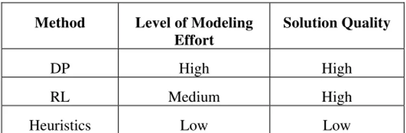
Reinforcement Learning is learning from interactions with an environment, from the consequences of action, rather than from explicit teaching. It is essentially a simulation-based dynamic programming [8] and is primarily used to solve Markov Decision Problems. Reinforcement Learning algorithms are methods for solving problems involving sequences of decisions in which each decision affects what opportunities are available later, in which the effects are generally stochastic. RL algorithms [3] may estimate a value function and use it to construct better and better decision making policies over time. The two most important distinguishing features of Reinforcement Learning are trial and error search and Delayed reward. Model-free methods of RL do not need the transition probability matrices and hence avoid the curse of modeling. RL stores the value function in the form of Q-factors. An MDP has millions of states. It uses the function approximation methods, such as Neural Networks, regression and interpolation, which need only a small number of scalars to approximate Q-factors of these states and hence avoid the curse of dimensionality. A comparison of DP, RL and Heuristic algorithms is shown in Table-I.

Table 1. Comparison of DP, RL & Heuristic Algorithms

Method Level of Modeling Effort

Solution Quality

DP High High RL Medium High Heuristics Low Low

Reinforcement Learning hence offers much scope in solving MDPs as it offers lesser modeling effort and high solution quality. This paper investigates a classical Markov Decision Problem using Reinforcement Learning concept.

2. n-Armed Bandit Problem

Consider a general learning problem where one faces repeatedly with a choice among n different options or actions. This is a classical MDP. After each choice a numerical reward is received from a stationary probability distribution that depends on the action selected. The objective is to maximize the expected total reward over a period of time. These types of problems are often referred to as an n-armed bandit problem so named by analogy to a “one armed bandit” having n levers.

In an n-armed bandit problem, each action has an expected or mean reward given that the action is selected. This is called the value of that action. One is encountered with the situation to choose an action depending on the value estimates. At any time there is at least one action whose estimated value is the greatest. This is called a greedy action. If you select a greedy action, then you are exploiting your current knowledge of the values of the actions. If you select one of the non-greedy actions, then you are exploring because this enables you to improve your estimate of the non-greedy action's value. Exploitation is the right thing to do to maximize the expected reward on the play, but exploration will produce the greater total reward in the long run. The selection of action thus may be exploring or exploiting. Various methods are used to assign a value to an action known as action value methods. Action Value methods are commonly used in Artificial intelligence, Robotics and Optimal Control applications.

3. Action Value Methods

Let us denote the true or actual value of an action ‘a’ as Q*(a), and the estimated value at the tth play as Qt(a).

The true value of an action is the mean reward received when that action is selected. This is estimated by averaging the rewards actually received when the action was selected. If at the tth play action ‘a’ has been chosen Ka times prior to t, yielding rewards r1, r2, r3, ……..rKa , then its value is estimated to be

a Ka t

K

r

r

r

a

greedy action selection rule is called -greedy method. An advantage of these methods is that, in the limit as the number of plays increases, every action will be sampled an infinite number of times, guaranteeing that





a

K

Simulations were carried out to assess the relative effectiveness of the greedy and -greedy methods, we compared them numerically on a suite of 3000 randomly generated n-armed bandit tasks with n=10. For each action, a, the rewards were selected from a normal probability distribution with mean Q*(a) and variance 1. The 3000 n-armed bandit tasks were generated by reselecting the Q*(a) 3000 times, each according to a normal distribution with mean 0 and variance 1 . We call this suite of test tasks the 10-armed testbed. Averaging over tasks, we plot the performance and behavior of various methods as they improve with experience over 2000 plays, as in Figures 1.1 – 1.4.

Fig. 1.1

Fig. 1.2

Fig 1.3

Fig 1.4

Figure 1.3 compares percentage optimal action and Figure 1.4 compares cumulative percentage optimal action for a greedy method with two -greedy methods ( = 0.01 and  = 0.2) on the ten armed testbed.

The -greedy methods eventually perform better because they continue to explore, and to improve their chances of recognizing the optimal action. The  = 0.2 method explores more, and finds the optimal action earlier, but never selects it more than 91% of the time.  = 0.01 method improves more slowly, but eventually performs better than the  = 0.2 method on both performance measures.

4. Modified Action Value Method

Although -greedy action selection is an effective and popular means of balancing exploration and exploitation in reinforcement learning, one drawback is that when it explores it chooses equally among all actions. This means that it is as likely to choose the worst-appearing action as it is to choose the next-to-best action. In tasks where the worst actions are very bad, this may be unsatisfactory. The obvious solution is to vary the action probabilities as a graded function of estimated value. The greedy action is still given the highest selection probability, but all the others are ranked and weighted according to their value estimates. These are called softmax action selection rules. The most common softmax method uses a Gibbs, or Boltzmann, distribution [14]. It chooses action on the tth play with probability

a Q_t

where  is a positive parameter called the temperature. The temperature  can be decreased over time to decrease exploration. High temperatures cause the actions to be all equi-probable. Low temperatures cause a greater difference in selection probability for actions that differ in their value estimates. In the limit as 0, softmax action selection becomes the same as greedy action selection. This method works well if the best action is well separated from the others, but suffers somewhat when the values of the actions are close.

4.1. Matlab Simulations

Softmax action selection also was carried out on the same 10-armed testbed on a suite of 3000 randomly generated n-armed bandit tasks and results consolidated in Figures1.5 to Figure 1.8. We used Boltzmann distribution and tested for temperatures  = 1, 0.2 and 0.01.

Fig. 1.5

Fig. 1.7

Fig. 1.8

The  = 0.01 method performs better and finds the optimal action earlier and is better than the  = 0.2 method on both performance measures. It was observed that the performance degraded at very low and very high temperatures.

5. Conclusion

Softmax action selection method performs better than the -greedy method as the average reward obtained and percentage optimal action are higher compared to -greedy methods. -greedy method is easy compared to softmax method as setting  value is easy. Selecting  value requires knowledge of the likely action values and of powers of e and also depends on the specific task.

References

[1] Barto, AG, Sutton, RS & Anderson, CW (1983) Neuron like elements that can solve difficult learning problems. IEEE Transactions on Systems, Man, and Cybernetics 13:834-846.

[2] Reinforcement Learning A Survey by Leslie Pack Kaelbling, Michael L. Littman and Andrew W. Moore Journal of Artificial Intelligence Research 4 (1996) 237-285.

[3] Reinforced Learning: An Introduction, Richard S. Sutton and Andrew G. Barto, A Bradford Book, The MIT Press, Cambridge, Massachusetts, London, England, 1998 ISBN 0-262-19398-1.

[9] Peter Dayan and Christopher JCH Watkins Reinforcement Learning, A Computational Perspective, Encyclopedia of Cognitive Science, John Wiley & Sons, 2006, DOI: 10.1002/0470018860.s00039.

[10] Classic and Heuristic Approaches in Robot Motion Planning – A Chronological Review, Ellips Masehian, and Davoud Sedighizadeh, World Academy of Science, Engineering and Technology 29 2007.

[11] Dimitri P. Bertsekas. Dynamic Programming and Optimal Control. Athena, MA, ISBN 1-886529-30-2, Vol. II, 3rd Edition, 2007. [12] Abhijit Gosavi "Reinforcement Learning: A Tutorial Survey and Recent Advances." INFORMS Journal on Computing, Vol 21(2), pp.

178-192, 2009.

[13] M. Hauskrecht. Value-function approximations for partially observable Markov decision processes. Journal of Artificial Intelligence Research, 13: 33{94, 2000}.

[14] Csaba Szepesvari, Algorithms for Reinforcement Learning, Synthesis Lectures on Artificial Intelligence and Machine Learning, Morgan & Claypool Publishers, 2010.

[15] Advances in Reinforcement Learning, Abdelhamid Mellouk, Published by InTechJaneza Trdine 9, 51000 Rijeka, Croatia, ISBN 978-953-307-369-9.

[16] Rebecca M. Jones, Leah H. Somerville, et al, Behavioral and Neural Properties of Social Reinforcement Learning, The Journal of Neuroscience, Sept 2011. JNEUROSCI.2972-11.2011.

[17] Reinforcement Learning in Professional Basketball Players, Tal Neiman & Yonatan Loewenstein, Nature Communications 2, Article Number 569, December 2011. DOI:10.1038/ncomms1580.