Maria Inês A. Vicente
Dissertation presented to obtain the
Ph.D. degree in Biology | Neuroscience
Instituto de Tecnologia Química e Biológica António Xavier | Universidade Nova de Lisboa
Maria Inês A. Vicente
Dissertation presented to obtain the
Ph.D. degree in Biology | Neuroscience
Instituto de Tecnologia Química e Biológica António Xavier | Universidade Nova de Lisboa
Oeiras,
Uncertainty in olfactory
decision-making
Acknowledgments
Zach. The freedom to believe that everything is possible. André. The eternal arm swirling mermaids.
Patricia. The companionship and shared growth. Gil. The space for naturality.
Rita. The possibility of the un-limit. The lab. The support and openness. Masa. The first steps.
Eric. The valuable discussions.
Zach, Rui. Marta, Susana. The opportunity to grow-up with you. Alfonso, Joe. The guidance.
PGCN 2007. Patricia, Rodrigo, Margarida, Zé, Mariana, Pedro, Patricio, Íris, Isabel. The time for dreams, magic and adventures. Margarida, Rodrigo, Zé. The simple truths.
Catarina. The digressions that kept me on track. Mãe, Pai, André, Avó, Família. O incondicional. Emília, Zé. O carinho.
Zazu, Pimenta, Buga. A sensibilidade. Zé. Pela nossa estrada.
Resumo
As relações entre precisão e velocidade em tomadas de decisão,
ou relações velocidade-precisão (speed-accuracy tradeoff, SAT),
têm sido estudadas extensivamente. No entanto, existe alguma
variabilidade nos valores de SAT observados entre estudos, e as
causas que poderão estar na origem desta variabilidade são ainda
desconhecidas.
Diversas explicações têm sido sugeridas, incluindo motivação ou
incentivo para velocidade vs. precisão, espécie ou modalidade
sensorial. No entanto, nenhuma destas hipóteses foi ainda testada
directamente. Uma explicação alternativa seria que os diferentes
graus de SAT obervados estariam relacionados com a tarefa que
está a ser desempenhada. Neste estudo, abordámos este problema
através da comparação de SAT em duas tarefas comportamentais
baseadas em odores, idênticas excepto na natureza da incerteza
associada a cada tarefa: uma tarefa de categorização com misturas
de odores, onde a informação relevante é manipulada variando o
grau de semelhança entre os estímulos que compõem a mistura; e
uma tarefa de identificação com odores puros, na qual a
informação relevante é reduzida diminuindo a intensidade dos
estímulos num gama de três passos logarítmicos.
Observámos que a duração de amostragem do odor (odor
comparação com a de categorização. Esta observação foi também
verificada quando as duas tarefas foram combinadas, intercalando
o conjunto de estímulos das tarefas de categorização e
identificação bem como misturas intermédias. Estas duas
manipulações interagiram de forma linear em relação ao OSD,
sendo consistente com a ideia de que concentrações baixas de
odores e contrastes reduzidos de misturas colocam fontes
independentes de incerteza.
Baseado nestas observações, formulámos a hipótese de que na
identificação de odores, a performance é limitada pela incerteza
do estímulo, ao passo que na categorização de misturas, a
performance é limitada pela variabilidade no mapeamento do
estímulo a resposta, que vai sendo aprendido sequencialmente, a
casa tentativa. Dada esta hipótese, investigámos se esta
aprendizagem teria uma influência diferente na escolha dos
animais na identificação de odores ou na categorização de
misturas. Verificámos, em ambas as tarefas, uma actualização da
escolha dos animais a cada tentativa. Contudo, enquanto que na
tarefa de categorização o viés na escolha dos animais aumentou
com a dificuldade da tentativa anterior e do respectivo resultado,
na tarefa de identificação este viés dependeu apenas da identidade
do odor e do resultado.
Em seguida, utilizámos uma estratégia de modelação para
investigar que mecanismos computacionais poderiam explicar as
mudanças comportamentais observadas na tarefa de identificação.
ser descritos tanto por modelos com e sem integração temporal,
colocando em perspectiva o uso generalizado de modelos de
integração para explicar tanto a escolha como o tempo de resposta
numa gama alargada de tarefas de decisão baseadas em percepção
(perceptual decision-making).
Finalmente, explorámos o papel da incerteza temporal em tarefas
de decisão baseadas em percepção, olhando para o impacto no
OSD da expectativa em relação ao início do estímulo.
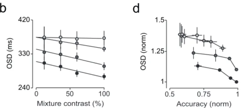
Observámos uma relação linear entre a média e o desvio padrão
de OSD para os diferentes constrastes de misturas e concentrações
de odores, consistente com a lei de Weber no domínio temporal.
Para ambas as tarefas, a média de OSD foi menor quando o início
do estímulo foi mais tardio (expectativa elevada). Esta diminuição
foi acompanhada por um decréscimo proporcional do desvio
padrão, tal como é previsto pela propriedade de escalonamento de
estimativa temporal para diferentes condições de expectativa
temporal. Verificámos que a magnitude desta componente
sensível a expectativa está correlacionada com a dificuldade do
estímulo, sendo que variações maiores no OSD correspondem a
valores menores de performance. Estes resultados demonstram
que o OSD é modulado por componentes não sensoriais, como a
expectactiva temporal, sugerindo que os tempos de reacção são
uma combinação entre processos de tomada de decisão e
mecanismos relacionados com atenção que são, por sua vez,
Abstract
Relationships between accuracy and speed of decision-making, or
speed-accuracy tradeoffs (SAT), have been extensively studied.
However, the range of SAT observed varies widely across studies
for reasons that are unclear. Several explanations have been
proposed, including motivation or incentive for speed vs.
accuracy, species and modality but none of these hypotheses has
been directly tested. An alternative explanation is that the
different degrees of SAT are related to the nature of the task being
performed. Here, we addressed this problem by comparing SAT
in two odor-guided decision tasks that were identical except for
the nature of the task uncertainty: an odor mixture categorization
task, where the distinguishing information is reduced by making
the stimuli more similar to each other; and an odor identification
task in which the information is reduced by lowering the intensity
over a range of three log steps. We found a much larger increase
in odor sampling duration (OSD) with difficulty for stimulus
detection compared to categorization. This was also observed
when the two tasks were combined, by interleaving the full set of
stimuli from the categorization and identification tasks as well as
intermediate mixtures. These two manipulations interacted
linearly with respect to OSD, consistent with the idea that low
concentrations and low mixture contrast pose independent sources
accuracy is limited by stimulus uncertainty, whereas in mixture
categorization, accuracy is limited by variability in the mapping
of the stimulus to the response, which must be learnt on a trial-by
trial basis. Given this hypothesis, we investigated whether
ongoing learning has a different influence on the choice of
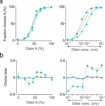
animals in identification and categorization. In both tasks there
was a clear trial-by-trial updating of the animal’s choice function.
However, whereas in categorization choice bias increased with
difficulty of the previous trial and outcome, in identification this
bias was dependent only on choice side and outcome.
Next, we used a modeling approach to investigate which
computational mechanisms might account for the behavioral
changes observed in the identification task. Interestingly, we
observed that our results were well described both by models with
and without temporal integration, putting into perspective the
generalized use of integrator models to explain choice behavior
and response times across a wide range of perceptual
decision-making tasks.
Finally, we explored the role of temporal uncertainty in
perceptual decision-making, by focusing on the impact of
stimulus onset expectation on OSD. We observed a linear
relationship between the mean and standard deviation of OSD
across mixture contrasts and odor concentrations, consistent with
Weber’s law in the temporal domain. For both tasks, mean OSD
was smaller for longer onsets (higher expectation), and this
standard deviation, as would be expected from the scalar property
of interval timing for different temporal expectation conditions.
The magnitude of this expectation-sensitive component was
correlated with stimulus difficulty, with lower accuracies
displaying larger changes in OSD. These results showed that
OSDs are modulated by non-sensory components such as
temporal expectation, suggesting that reaction times are a
combination between decision-making processes and
attention-related mechanisms that are affected by time estimation
Abbreviations list
5-HT Serotonin
AFC Alternative forced-choice
BeT Behavioral theory of timing
CV Coefficient of variation
DDM Drift-diffusion model
DRN Dorsal raphe nucleus
DV Decision variable
EEG Electroencephalography
fMRI Functional magnetic resonance imaging
IT Inferotemporal cortex
LeT Learning-to-time
LIP Lateral intraparietal area
M Magnocellular
MC Mitral cells
MT Middle temporal visual area
OB Olfactory bulb
OC Olfactory cortex
OFC Orbitofrontal cortex
ORN Olfactory receptor neuron
OSD Odor sampling duration
OT Olfactory tubercle
P Parvocellular
PC Piriform cortex
RL Reinforcement learning
RT Reaction time
SA Sequential analysis
SAT Speed-accuracy tradeoff
SD Standard deviation
SDT Signal detection theory
SET Scalar expectancy theory
ST Scalar timing
Figure Index
Figure 2.1 | Stimulus design for the different behavioral tasks ...28
Figure 2.2 | PID signal for different odor concentrations ...29
Figure 2.3 | Two-alternative odor choice task...31
Figure 3.1 | Comparison between odor mixture categorization and odor identification tasks – session and rat data...40
Figure 3.2 | Comparison between odor mixture categorization and odor identification tasks – population data ...41
Figure 3.3 | Movement time for odor mixture categorization and odor identification tasks...42
Figure 3.4 | Odor mixture categorization with lower contrast stimuli ...43
Figure 3.5 | Odor mixture identification task...45
Figure 3.6 | Trial-by-trial learning ...46
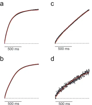
Figure 4.1 | Exponential fit of the odor temporal profiles for different concentrations ...56
Figure 4.2 | Model structure...57
Figure 4.3 | Drift-diffusion model with constant input (Model 1) ...66
Figure 4.4 | Drift-diffusion model with time-varying input from exponential fit of mean odor time-courses (Model 2) ...69
Figure 4.6 | Model with no temporal integration and time-varying input from exponential fit of mean odor time-courses (Model
4) ...72
Figure 4.7 | Evidence-accumulation model with diffusion coefficient set to zero and constant input (Model 5)...73
Figure 4.8 | Evidence-accumulation model with diffusion coefficient set to zero and time-varying input from exponential fit of mean odor time-courses (Model 6) ...74
Figure 4.9 | Model with no temporal integration, diffusion coefficient set to zero and time-varying input from exponential fit of mean odor time-courses (Model 7) ...76
Figure 4.10 | Model with no temporal integration, diffusion coefficient set to zero and time-varying input from single-trial odor time-courses (Model 8) ...77
Figure 4.11 | Model 1 with Gaussian variability in non-decision time (Model 9) ...80
Figure 4.12 | Model 2 with Gaussian variability in non-decision time (Model 10) ...81
Figure 4.13 | Model 3 with Gaussian variability in non-decision time (Model 11) ...82
Figure 4.14 | Model 4 with Gaussian variability in non-decision time (Model 12) ...83
Figure 4.15 | Drift-diffusion model fit to mean and standard deviation of reaction times...85
Figure 4.16 | Inhalation variability simulation...88
Figure 5.1 | Properties of reaction time distributions...96
Figure 5.2 | Effect of stimulus expectation on reaction times...98
Table Index
Table 4.1 | Model variants used to fit the behavioral data from the identification task...58
Table 4.2 | Best-fit parameter values from the different models (k,
sensitivity; β, scaling exponent; A, bound; tND, mean
non-decision time; σtND, standard deviation of non-decision time;
Acc, accuracy; mRT, mean reaction times; vRT, variance of reaction times; sdRT, standard deviation of reaction times)67
Author contributions
Maria Inês Vicente (MIV), André Gil Mendonça (AGM) and
Zachary Frank Mainen (ZFM) designed the experiments (Chapter
2). MIV and ZFM designed the model (Chapter 4). MIV
conducted the experiments with assistance from AGM. MIV
analyzed the data and implemented the model (Chapters 3, 4 and
5).
Part of the work presented in Chapters 2 and 3 has been submitted
Contents
Acknowledgments i
Resumo ii
Abstract v
Abbreviations list viii
Figure Index x
Table Index xii
Author contributions xiii
Contents xiv
1 General Introduction 1
1.1 Introduction 2
1.2 Perceptual decision-making 3
1.2.1 Conceptual framework for studying perceptual decision-making 3
1.2.2 Theoretical framework for studying perceptual decision-making 4
1.3 Sources of uncertainty in decision-making 7
1.3.1 Speed-accuracy tradeoffs 7
1.3.2 Bridging perceptual and economic decision-making 11 1.4 Temporal uncertainty in perceptual decision-making 14
1.4.1 Interval timing 15
1.4.2 Models of interval timing 16
1.4.3 Temporal expectation 18
1.5 Objectives and organization of the thesis 21
2 Odor identification and odor mixture categorization tasks 22
2.1 Introduction 23
2.2 Animal subjects 25
2.3 Testing apparatus and odor stimuli 26
2.4 Reaction time paradigm 30
2.5 Training 33
2.6 Statistical analysis 35
3 Speed-accuracy tradeoffs in olfaction 37
3.1 Introduction 38
3.3 Odor mixture identification task 43
3.4 Trial-by-trial learning 45
3.5 Discussion 47
4 A modeling approach for the study of the identification task 49
4.1 Introduction 50
4.2 Modeling framework approach 53
4.2.1 The diffusion model framework 53
4.2.2 Variants of the model 55
4.2.3 Model fitting 60
4.2.4 Inhalation variability 63
4.3 Model fitting results 64
4.3.1 Fitting mean reaction time and accuracy 65
4.3.2 An attempt to capture the reaction time distributions 78
4.3.3 Inhalation variability 85
4.4 Discussion 89
5 Temporal uncertainty in odor identification and mixture
categorization 92
5.1 Introduction 93
5.2 Properties of reaction time distributions 94
5.3 Temporal expectation 96
5.4 Discussion 103
6 General discussion 105
6.1 Overview of empirical findings 106
6.2 Sources of uncertainty in decision-making 108
6.2.1 Speed-accuracy tradeoff and the origin of decision noise 108
6.2.2 Post-decisional processes and learning 111
6.2.3 Decision response time and decision confidence 113 6.3 Olfactory coding: insights from neural circuits 115 6.3.1 Coding of odor intensity in the olfactory system 115 6.3.2 Recordings from the olfactory system: future directions117
6.3.3 Decision variables in the brain 120
6.4 Temporal uncertainty and decision-making: the multiple
shades of reaction times 123
1.1 Introduction
The evolution of sophisticated brains has given us the capacity for
flexible decision-making. The evidence we obtain through our
senses (or from memory) need not precipitate an immediate,
reflexive response. Instead our decisions can be deliberative and
conditional, contingent on other sources of information, long-term
goals, history and values.
A decision is a commitment to a categorical proposition and is
based on a variety of factors: quality of the evidence for a
particular option, prior knowledge concerning the relative merit of
the options, expected costs and rewards associated with the
possible decisions and their outcomes, and other costs associated
with gathering evidence (e.g., the cost of elapsed time). In
addition, decisions are always made in the face of uncertainty.
Both natural events in the world and the consequences of our
actions are fraught with unpredictability, and the neural processes
generating our percepts and memories may be unreliable and
introduce additional variability. Unraveling the relationship
between neural and behavioral variability is fundamental to
understanding how decisions are formed in the brain.
The present work has investigated the contributions of different
sources of uncertainty in perceptual decision-making, by
In the following sections, we will: review the conceptual
framework and quantitative models used to study perceptual
decision-making (1.2 Perceptual decision-making); consider the
contribution of different sources of uncertainty in perceptual
decision-making, while focusing on the relation between choice
behavior and response times across different perceptual
decision-making tasks (1.3 Sources of uncertainty in perceptual
decision-making); and explore the role of temporal uncertainty
on perceptual decision-making and the relationship between
decision-making and time estimation processes (1.4 Temporal
uncertainty in perceptual decision-making).
1.2 Perceptual decision-making
1.2.1 Conceptual framework for studying perceptual
decision-making
Perceptual decision-making is the process by which sensory
information is used to guide behavior toward the external world.
This involves gathering information through the senses,
evaluating and integrating it according to the current goals and
internal state of the subject, and using it to produce motor
responses1,2.
At any given point in time, the state of the world must be inferred
based on the noisy data provided by the sensory systems, and
behavior is critically dependent on the ability to quickly and
instance, deciding whether or not a predator is present in a
shadowy corner will dictate an animal’s subsequent action and
survival. Various factors must be taken into account before
committing to a decision and executing the appropriate behavioral
response. These include the quality of the evidence derived from
the sensory observations; prior history, which determines the
predicted probability of seeing a particular stimulus or receiving a
particular reward in the future3–6; and value, the subjective costs
and benefits that can be attributed to each of the potential
outcomes of the decision process. These different sources of
information are then accrued into a quantity – the decision
variable (DV) – that is then interpreted by the decision rule to
produce a particular choice1. A conceptually simple rule is to
place a criterion value on the DV. Like this, the magnitude of the
DV reflects the balance of support/opposition for a given choice,
allowing the decision maker to achieve different goals, including
maximizing accuracy or reward or achieving a target decision
time1. Post-decisional processes also play a critical role in shaping
future decisions, namely via learning mechanisms mediated by
the evaluation, or performance monitoring, of the choice with
respect to its particular goals5,7.
1.2.2 Theoretical framework for studying perceptual
decision-making
The quantitative study of perception, or psychophysics, has
18608,9. Since then, different mathematical descriptions have been
proposed to better test and understand perceptual
decision-making, namely signal detection theory (SDT) and sequential
analysis (SA).
SDT is one of the most widely used formalisms to study
perception10,11. It prescribes a process where performance of
perceptual tasks reflects not just the inherent sensitivity of the
subject to the relevant stimuli but also how the subject uses that
information to generate a choice. According to SDT, the
decision-maker obtains an observation of noisy evidence from the
stimulus, which gives rise to the DV that is then evaluated
according to the decision rule. In simple binary decisions, the DV
is typically related to the likelihood ratio of the different
alternatives, and then compared to a criterion. This criterion can
also incorporate different priors and value, allowing SDT to
provide a flexible framework to form decisions and achieve a
variety of goals1,12.
SA is a natural extension to SDT that accommodates multiple
pieces of evidence observed over time. Conceptually, the idea is
that in the presence of uncertainty or noise, the decision maker
can benefit from sampling multiple times from the noisy
distribution of values representing the stimulus. After each
acquisition, a DV is calculated from the evidence obtained up to
that point and compared to the decision rule, normally represented
by a positive and negative criterion, which correspond to each
criterion bounds, the bound that is first reached determines the
decision and response time of the decision maker. There are
several instantiations of sequential sampling models1,13–19. For
example, in random walk models, the DV is a cumulative sum of
evidence over discrete time steps. If the evidence is the logarithm
of the likelihood ratio, then this process corresponds to the
statistically-optimal Sequential Probability Ratio Test20, which
anecdotally played a prominent role in World War II allowing to
break the German enigma cipher21,22. Instead, if the evidence is
sampled from a Gaussian distribution in infinitesimal time steps,
the process is termed diffusion with drift or bounded diffusion.
While many models provide an account of either RT14,23 or
accuracy (SDT10), sequential sampling models relate shapes of
RT distributions with probabilities of correct and incorrect
responses, thereby explaining how RT and choice accuracy jointly
vary as a function of the experimental conditions of interest.
The parameters of these sequential sampling models allow
quantifying several latent psychophysical processes, namely the
speed of sensory information processing, given by the rate of
accumulation; response caution, from the bound height; and the
amount of time spent on processes unrelated to decision
formation.
In recent years, integrator models have gained prominence in the
field of decision-making due to its ability to explain several
features of behavioral and neural data. First, they have described
including perceptual discrimination and value-based choices24–29.
Second, they can be tuned to fit task conditions, such as reward
ratios or prior probability30–32. And third, these models have been
used to explain neurophysiological data1,33 and recordings of
neural activity in primates have shown neural correlates
resembling the DV34.
1.3 Sources of uncertainty in decision-making
1.3.1 Speed-accuracy tradeoffs
The relationships between accuracy and speed of
decision-making, or speed-accuracy tradeoffs (SATs), have been
effectively modeled as integration of sensory information to a
bound13,25,34–37. Speed and accuracy in perceptual decisions show
characteristic relationships and there are at least three
psychophysical experimental contexts in which the relationship
between speed and accuracy has been studied: 1) sampling time
manipulation: when the experimenter limits the duration of the
stimulus and/or sets a deadline for response time, performance
accuracy decreases with shorter sampling times; 2)
speed-accuracy tradeoff: when subjects are instructed to perform
rapidly, accuracy drops; conversely, when instructed to emphasize
accuracy, performance slows (traditionally, this is the technical
definition of ‘speed-accuracy tradeoff’); 3) difficulty effects:
when a participant is free to choose when to respond (a reaction
The random-dot motion discrimination (RDMD) task, which has
been extensively studied in the field of perceptual
decision-making, is a good example of a task where SAT has been
observed and how this relationship can be well explained by
integrator models. In this task, participants are presented with a
field of flickering dots, some of which move randomly and some
of which move coherently in one of two possible directions, and
asked to report the net direction of motion. The difficulty of the
task is changed by manipulating the fraction of coherently moving
dots. SAT and the impact of temporal integration in this task have
been investigated in humans and monkeys in two ways. First, by
varying the viewing time and measuring the discrimination
threshold for each duration, it was shown that sensitivity increases
with viewing times up to ~2 s39,40. Then, in a reaction time (RT)
version of this task, it was found that as motion coherence was
decreased, RTs increased from 300 to >800 ms25,34. Moreover,
these data could not only be fit quantitatively with a simple
diffusion model25, but neurophysiological recordings and
manipulations also provided strong evidence sustaining the idea
of a neural integrator that underlies the decision process34,41–43.
Recordings from the parietal cortex (the lateral intraparietal area,
LIP) showed that neuronal activity ramps up at a rate correlated
with the strength of the motion signal until it reaches a level that
is constant across motion strengths, as if a decision threshold was
reached34,42,44–46. This pattern of firing matches quite closely to
what is expected of the DVs posited by integrator models45,47.
state of the DV provided added evidence supporting the integrator
model as a substrate of the decision process48,49.
In addition to the studies using the RDMD task and performed in
humans and monkeys, SATs have been extensively studied across
different tasks, modalities and species, including rodents and
insects1,13,25,34,36,38,50–58. However, the range of SATs observed
varies widely across studies for reasons that are unclear. For
example, reported increases in RT with increased difficulty of
perceptual discrimination range from over 500 ms in humans25
and monkeys34 performing the RDMD task, to 100 ms in mice
performing a visual contrast detection task55, to less than 30 ms in
rats performing an odor mixture discrimination task52.
In particular, studies of odor discrimination in rodents have
reported SATs of different magnitudes52–54. Uchida and Mainen
(2003)52 used a two-alternative forced-choice (2-AFC) task in
which eight different binary odor mixture stimuli were randomly
interleaved and rewarded according to a categorical boundary. As
mixture ratios approached the category boundary, choice accuracy
dropped to near chance, yet odor sampling time increased only 30
ms52. On the other hand, Abraham et al. (2004)53, using a
go/no-go odor paradigm where odor mixture stimuli were presented in
blocks of trials, reported that for a high level of accuracy, mice
took an additional time of 70-100 ms to discriminate closely
related mixtures. In addition, in mice performing a 2-AFC where
the duration of odorant sampling was controlled by the
Rinberg et al. (2006)54 observed an improvement in performance
as a function of stimulus duration across different mixture
difficulties.
These apparent discrepancies were interpreted as a manifestation
of SAT in olfaction59, where speed had been favored over
accuracy in the study from Uchida and Mainen (2003)52, and the
opposite in Abraham et al. (2004)53 and Rinberg et al. (2006)54
(accuracy had been privileged at the expense of speed).
However, in a further twist, Zariwala et al. (2013)56, by
performing a large battery of variants of the categorization task
from Uchida and Mainen (2003)52, suggested an alternative
explanation for the differences amongst these tasks that was not
based on differences in SAT. According to this study, the higher
accuracy reported in Abraham et al. (2004)53 and Rinberg et al.
(2006)54 could be attributed to the use of blocked rather than
interleaved stimulus difficulties, which leads to a better
anticipation of stimulus identity. The greater change in RTs with
difficulty reported by Abraham et al. (2004)53 could be explained
by the effect of reward expectation on response speed. And
finally, the increase in performance as a function of stimulus
duration reported in Rinberg et al. (2006)54 could be explained by
the increase of go-signal anticipation over time (i.e. increase in
hazard rate) stemming from the temporal statistics of the uniform
distribution used for the go-signals in this study. In agreement
with this, when Zariwala et al. (2013)56 performed a similar
constant the time of go-signal within a block, hence not changing
the anticipation, they failed to observe an increase in accuracy
when the amount of time at the odor port augmented.
Together these results highlight a dissociation of accuracy from
RT in the odor mixture categorization task56, suggesting that the
noise related with the stimulus is not the dominant source of
uncertainty. Which other sources of uncertainty could then be
limiting performance in the mixture categorization task?
1.3.2 Bridging perceptual and economic decision-making
There is a common structure to virtually all decision-making tasks
employed across the literature: an agent is required to identify one
or more stimuli in a given sensory modality (what is it?), and then
to select a response which will maximize the probability of
positive feedback or reward (what is it worth?).
Perceptual decision-making, as described above, is concerned
with how observers detect, discriminate, and categorize noisy
sensory information. Because uncertainty in perceptual
decision-making tasks is assumed to be due to the noise associated with the
stimulus, these experiments often take place in a constant stage of
task performance, where the stimulus-response-reward
contingencies have been learnt through extensive training, and
learning is thought to be stationary. Thus, the computational
models that have been used to characterize performance have
reinforcement learning that occurs following feedback60. In the
standard model of perceptual decision-making, based on the
discrimination of motion direction of randomly moving dots61,
sensory neurons in the middle temporal visual area (MT) vote
with their firing rates for the perceived direction of motion and
their responses are then weighted, summed, and passed through a
binary decision function. In this model, behavioral variability
mainly arises through noise introduced in the responses of the
individual neurons. Sequential sampling models, as described
above, are an example of this kind of architecture, where choices
depend on a serial sampling mechanism, in which evidence about
the identity of the stimulus is collected and integrated until a
criterion level of certainty is reached20,37,62.
However, all perceptual decisions are ultimately motivated by
reward (or the avoidance of loss). Indeed, there are examples in
the literature focusing on how reward might influence sensory
discrimination30,32,63–65 and showing that rewards (or informative
feedback) play a role on learning about sensorimotor acts5,7,66,67.
This implies that, although perceptual decision-making tasks have
focused on the optimization of detection or categorization
judgments guided by sensory stimuli, subjects are swayed by
factors mediated by reinforcement statistics. Hence, the
environmental structure and the way it influences the tradeoff
between information and reward acquisition should also be
considered for the assessment of choice optimality60. In
agreement with this idea, recent work has shown that, in a visual
not only the visual responses to the current stimulus but also a
bias and history term depending on the outcome of the previous
trial7.
The field of decision-making that is concerned with how subjects
choose among different options on the basis of their associated
reinforcement history is economic decision-making. In contrast to
perceptual decision-making, economic decision-making tasks
tend to employ stimuli that are perceptually unambiguous but
associated with distinct reward statistics, where the uncertainty is
derived from variability in internal information about the
expected value of each option. One very successful class of
models used in economic decision-making, that draws upon a rich
literature from learning theory in experimental psychology68 and
machine learning69, is reinforcement learning (RL), which
describes the mechanisms by which the value of stimuli or actions
is learned. RL proposes that these values are updated according to
how surprising an outcome is – a prediction error – scaled by a
further parameter that controls the rate of learning. Recently, the
RL framework has been successfully applied to a perceptual
decision-making task to explain improvements in perceptual
performance67. In monkeys trained on a visual motion
discrimination task, improvements in perceptual sensitivity were
shown to correspond to changes in motion-driven responses of
neurons in area LIP, which represents the readout to motion
information to form a direction decision, but not area MT, a likely
source of that motion information70. These changes were well
sensory neurons and LIP-like decision neurons were adjusted
according to a prediction error signal67. Evidence from
neurophysiological recordings, namely from parietal cortex, basal
ganglia and orbitofrontal cortex (OFC), have also supported this
bridge between perceptual and economic-decision making60.
1.4 Temporal uncertainty in perceptual decision-making
Animals live in naturally complex, ever-changing environments,
where identifying temporal regularities is extremely important,
enabling them to predict behaviorally relevant events. Hence, to
behave adaptively in these environments, animals must not only
learn which actions to take in a particular context given their past
experience, but also to learn the temporal information about when
those actions and the respective consequences occur.
Time is a fundamental dimension of animals’ experience in the
world. As such, temporal information provided by stimuli that
predict salient events can be shown to exert a powerful influence
on the organization of behavior, suggesting that the computation
1.4.1 Interval timing
Time is not sensed through a sensory epithelium, but timing is
key to many aspects of behavior, especially foraging and learning.
Importantly, interval timing exhibits regularities that mimic those
of traditional sensory systems. The best known is a strong version
of Weber’s law (i.e., the just noticeable difference is proportional
to the baseline for comparison73) known as scalar timing (ST)74,75.
For example, in a typical duration reproduction procedure, known
as ‘peak-interval procedure’, when participants are asked to
reproduce a criterion interval that was previously learnt, the
responses typically distribute around the criterion interval with a
width that is proportional to the temporal criterion. Moreover, the
relative trial-to-trial response variability, e.g., the coefficient of
variation (CV) associated to the estimation of different intervals,
appears to be constant regardless of the estimated time74,76.
Remarkably, not only the CV, but also the entire distribution of
timed responses is scale invariant, i.e., identical when plotted as a
function of time relative to the mean. The ST property holds for
many species and over a broad range of temporal intervals74,75,
suggesting that ST reflects something fundamental about the way
organisms structure their behavior in time. In addition, it
represents a very strong quantitative constraint on the neuronal
1.4.2 Models of interval timing
Traditional sensory modalities such as vision, audition or
olfaction are processed by known sensory organs and brain areas.
Time perception, on the other hand, still lacks a clear and direct
demonstration of how it would be implemented within the
nervous system. Whether the representation of temporal
information is instantiated within a dedicated timing network, or
distributed across different brain areas as a common property of
many or all neural systems, is still a matter of debate and ongoing
research77.
Neurally-inspired models have suggested different encoding
schemes for time related information, namely oscillatory or
periodic activity in neural circuits78,79, integration of noisy firing
of neural populations80 and state-dependent changes in network
dynamics81.
Additionally, several abstract models of how animals track the
passage of time have been proposed, many of which fall in one of
two categories: accumulator models tell time by counting pulses
emitted by a pacemaker and comparing it to a remembered value
(Scalar expectancy theory, SET76), while state based models
represent time as a trajectory progressing through a sequence of
states (Behavioral theory of timing, BeT82; Learning-to-time,
LeT83).
SET is based on an internal clock model, in which pulses that are
accumulator. During training, at the time of reward or feedback,
the number of pulses that have been received from the
accumulator is stored in reference memory. For test trials, the
response is controlled by the ratio comparison between the current
subjective time/clock reading – stored in the accumulator – and a
sample taken from the distribution of remembered criterion
durations, which are represented as the number of pulses from
previously reinforced clock readings stored in reference memory.
In this framework, the scalar property derives from the
assumption that the accumulation error is proportional to the
criterion duration76,79,84.
BeT (as well as LeT, a derivative of BeT) emphasizes the role of
behavior in temporal discrimination82,85. According to this theory,
certain kinds of adjunctive or superstitious behaviors, such as
turning, scanning a corner, hopper inspection, occur in a
consistent fashion such that they are temporally related to
reinforcement delivery. These kinds of behavior may then act as
conditional discriminative stimuli when an animal is required to
make a temporal discrimination. Formally, these classes of
adjunctive behavior correspond to hypothetical states, whose
transitions are driven by pulses from a hypothetical pacemaker
described by a Poisson process, with a rate proportional to the
reinforcement rate. The question that is then asked is: what is the
probability that an animal is in state n at time t? Varying the rate
of reinforcement will generate distributions of behavior whose
Recent work has suggested a hybrid model between SET and
LeT, that preserves the overall learning structure of LeT but
replaces its state-activation dynamics by a scalar-inducing
dynamics equivalent to the pacemaker-accumulator structure of
SET86.
1.4.3 Temporal expectation
Our sensory systems are consistently being exposed to a rich and
rapidly changing scenery. To cope with the overwhelming amount
of stimulation, we constantly generate and update expectations
about critical events, such as the onset of behavioral relevant
stimuli, in order to optimize our interaction with unfolding
sensory stimulation. Temporal anticipation has been generally
studied by manipulating stimulus predictability through the
hazard rate, which specifies the likelihood of a stimulus
appearing, given it has not appeared so far. A long tradition of RT
experiments has documented that RT decreases as the stimulus
becomes more likely. These findings have been interpreted to
show that observers implicitly learn to use changes in stimulus
likelihood to change RTs87–89. And what are the underpinnings of
the effects of temporal expectation on RT? Research in this field
has revealed that the temporal prediction of events has pervasive
effects in modulating perception and action90.
The ability to extract temporal patterns and regularity of events
execution90. Early behavioral studies in humans have led to the
general interpretation that stimulus predictability mainly changes
the willingness of the subjects to respond13,91. A more recent
study, using sequential sampling models to analyze the observed
temporal expectation effects on task performance, showed that
temporal prediction mainly affects the duration of non-decision
processes92. In addition, electrophysiological recordings in
monkeys revealed systematic changes in neural firing patterns as
a function of temporal expectation in motor-related regions89,93–97.
For instance, in primary motor cortex, neurons become more
synchronized around the expected time of an imperative
go-signal93; and in LIP, which has also been implicated in perceptual
decision-making, saccade-related activity varies according to the
evolving temporal conditional probability for the appearance of
the task-relevant target89,97. Electroencephalography (EEG) and
neuroimaging studies in humans have supported the interpretation
that temporal expectancies modulate motor-related processese.g.,98–
101
.
However, the effects of temporal prediction are not confined to
motor-related variables. The temporal certainty between events
can modulate perceptual thresholds for detecting visual
features102,103 and increase perceptual processing104–106, namely by
improving the quality of sensory information, as revealed by a
diffusion model-based analysis106. However, response criteria
adjustments were also shown to be responsible for behavioral
performance improvements107. Moreover, it has been
rhythmic motor activity108–112. Electrophysiological recordings
showed that temporal expectation modulates neuronal activity in
the visual cortex of monkeys, namely in V1113,114, V4115, MT116
and inferotemporal cortex (IT)117, and in the primary auditory
cortex of rats118. In humans, EEG and neuroimaging studies have
also implicated sensory-related areas in temporal
predictability99,119,120.
As it is not yet clear how time perception is implemented in the
brain, these studies demonstrate that there is also not a consensus
about the impact of temporal expectation in modulating sensory
processing and motor-related variables.
There has been the suggestion that the mechanisms that underlie
temporal processing are also shared by perceptual
decision-making processes80,121,122. Evidence has shown that time is
represented in the form of a hazard function by the same type of
neurons that represent a DV in area LIP89,97. In addition, the scalar
property between the mean and SD of responses times is also
predicted by diffusion models123. Interestingly, it was also
proposed that time estimation can be explained by a bounded
accumulation mechanism80. In future research, the use of properly
designed tasks that allow manipulating independently the
variables associated with the axes of perceptual decision-making
(e.g., stimulus uncertainty) and time estimation (e.g., hazard rate),
and evaluating how RT and accuracy are jointly modified, will
give further insight about the relationship between perceptual and
1.5 Objectives and organization of the thesis
The present work has focused on the contributions of different
sources of uncertainty in perceptual decision-making, in particular
in the relationship between speed and accuracy.
In Chapters 2 and 3 we took a behavioral approach to
investigate what accounts for the different degrees of SAT
observed across behavioral studies. Our approach was to compare
SAT in odor-guided decision tasks that would pose different
sources of uncertainty for the brain. A first objective was to
develop an olfactory task that would display a robust degree of
SAT to be then compared to the previously described mixture
categorization task52. Chapter 2 describes the behavioral tasks
used to study this problem (odor identification and odor mixture
categorization tasks) and how the data was analyzed. The
behavioral results are presented in Chapter 3.
In Chapter 4 we used a modeling approach to study the
computational mechanisms that underlie the behavioral changes
observed in the odor identification task developed in the previous
chapters.
In Chapter 5 we explored the role of temporal uncertainty in
perceptual decision-making. More specifically we investigated the
impact of the temporal expectation about stimulus onset on
2
Odor identification and odor
2.1 Introduction
Relationships between accuracy and speed of decision-making, or
speed-accuracy tradeoffs (SATs), have been extensively studied
in humans and other species including monkeys, rodents and
insects1,13,25,34,38,50–57. However, the range of SAT observed varies
widely across studies for reasons that are unclear. For example,
reported increases in RT with increased difficulty of perceptual
discrimination range from over 500 ms in humans25 and
monkeys34 performing a RDMD task, to 100 ms in mice
performing a visual contrast detection task55, to less than 30 ms in
rats performing an odor mixture discrimination task52. It is not
known what accounts for such different degrees of SAT observed
across different studies.
Motivation for speed vs. accuracy is thought to be a key
parameter affecting SAT59 and is a possible explanation for the
differences observed across similar studies showing SAT of
smaller52 or larger53,54 magnitudes. Two alternative possibilities
are that longer SAT tradeoffs reflect neural mechanisms that are
species-specific or sensory modality-specific. An additional
possibility is that SAT differences arise from differences in the
underlying computational requirements of different
decision-making tasks56. Given that species, modality, task structure all
vary across the different studies in question, these possibilities are
not possible to distinguish from existing data.
Our strategy was to compare SAT in two behavioral tasks that
task difficulty. The first was an odor mixture categorization task52
in which the difficulty was increased by making the stimuli closer
to a decision or category boundary. The second was an odor
identification task in which the difficulty was increased by
lowering stimulus concentration. Thus, by having the same
subjects performing two tasks that were different only for the set
of stimuli, and by holding species, modality and motivation, we
were in a condition that allowed us to test if SAT was dependent
on the nature of the task.
In comparison with visual and auditory stimuli, odors are harder
to control because of their intrinsic temporal dynamics124.
Nevertheless, the use of automated olfactometers52 has allowed a
tight control of stimulus conditions, namely controlling precisely
the time of odor delivery and guarantying the reproducibility of
odor amplitude and time-course125. In addition, odor temporal
profiles have been successfully used in models of the olfactory
receptor neurons124 (ORNs) and of the olfactory bulb125 (OB) to
predict physiological responses. In Chapter 4, we investigated the
contribution of the odor temporal profiles on the observed
behavioral data, showing that, in addition to vision and audition,
odor-guided tasks are also suitable to study the relationship
between time and choice in decision-making.
Below, we will depict the odor-guided behavioral tasks employed
2.2 Animal subjects
Four Long Evans rats (200-250 g at the start of training) were
trained and tested in accordance with European Union Directive
86/609/EEC and approved by Direcção-Geral de Veterinária
(DGV) of Portugal. Rats were trained and tested on three different
tasks: (1) a two-alternative choice odor identification task; (2) a
two-alternative choice odor mixture categorization task52; and (3)
a two-alternative choice “odor mixture identification” task. The
same rats performed all three tasks and all other task variables
were held constant. Each rat performed one session of 90-120
minutes per day (300–500 trials), 5 days per week for a period of
~120 weeks. Each task was tested independently in blocks of
sessions numbering 10–20 for odor identification and mixture
categorization tasks; 5–10 for odor mixture identification and
categorization with lower contrast stimuli. Rats were pair-housed
and maintained on a normal 12 hr light/dark cycle and tested
during the daylight period. Rats were allowed free access to food
but were water-restricted. Water was available during the
behavioral session and for 20 minutes after the session at a
random time as well as on non-training days. Water availability
was adjusted to ensure animals maintained no less than 85% of ad
2.3 Testing apparatus and odor stimuli
The behavioral apparatus for the task was designed by Z.F.M. in
collaboration with M. Recchia (Island Motion Corporation,
Tappan, NY). The behavioral control system (BControl) was
developed by Z.F.M, C. Brody (Princeton University) in
collaboration with A. Zador (Cold Spring Harbor Laboratory).
The behavioral setup consisted of a box (27 x 36 cm) with a panel
containing three conical ports (2.5 cm diameter, 1 cm depth)52.
Each port was equipped with an infrared
photodiode/phototransistor pair that registered a digital signal
when the rat‘s snout was introduced into the port (“nose poke”),
allowing us to determine the position of the animal during the task
with high temporal precision. Odors were delivered from the
center port and water from the left and right ports. Odor delivery
was controlled by a custom made olfactometer52 designed by
Z.F.M.. During training and testing the rats alternated between
two different boxes; the manifolds were changed every 2/3 days
and the correspondence between odor valve and stimulus
difficulty was not always the same.
The test odors were S-(+) and R-(-) stereoisomers of 2-octanol,
chosen because they have identical vapor pressures and similar
intensities. In the odor identification task, difficulty was
manipulated by using different concentrations of pure odors,
ranging from 10-4 to 10-1 (v/v) (Fig. 2.1b). The different
concentrations were produced by serial liquid dilution using
loaded in a different holder (Puradisc 13 Syringe Filter, 2.7 mm
pore size, #6823-1327, GE Healthcare), joining in a symmetric
manifold, about 10 cm from the odor port52. In the odor mixture
categorization task, we used binary mixtures of these two
odorants at different ratios, with the sum held constant: 0/100,
20/80, 32/68, 44/56 and their complements (100/0, etc.) (Fig.
2.1a). Difficulty was determined by the distance of the mixtures
to the category boundary (50/50), denoted as “mixture contrast”
(e.g., 80/20 and 20/80 stimuli correspond to 60% mixture
contrast). Choices were rewarded at the left choice port for
odorant A (identification task) or for mixtures A/B > 50/50
(categorization task) and at the right choice port for odorant B
(identification task) or for mixtures A/B < 50/50 (categorization
task). In both tasks, a set of eight stimuli was randomly
interleaved within the session. During testing, the probability of
each stimulus being selected on a given trial was the same.
(Fig. 2.1 continues in the next page)
Detection or Identification Categorization
a
Conc. A (v/v)
Conc.
B
(v/v)
10-4 10-3 10-2 10-1 10-4
10-3 10-2
10-1 b
Conc. A (v/v)
Conc.
B
(v/v)
10-4 10-3 10-2 10-1 10-4
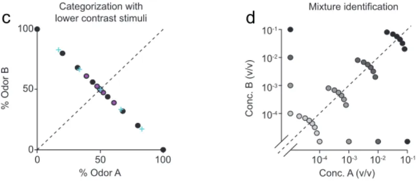
Figure 2.1 | Stimulus design for the different behavioral tasks
(a,b) Odor mixture categorization and odor identification tasks. In the mixture
categorization task, two odorants, (S-(+)-2-octanol and R-(-)-2-octanol), were mixed in different ratios – 0/100, 20/80, 32/68, 44/56 and their complements – presented at a fixed total concentration of 10-1, and rats were rewarded according to the majority component (a). In the odor detection or identification task, the same odorants were presented independently at concentrations ranging from 10-1 to 10-4 (v/v) and sides rewarded accordingly (b). Dot shading represents odor concentration, with highest concentration corresponding to the darkest shade. (c) Comparison between the different datasets used for the mixture categorization task. Black circles same as in (a). Blue crosses represent the set of stimuli with the following mixture ratios: 0/100, 17/83, 33.5/66.5, 50/50; magenta circles: 0/100, 39/61, 47.5/52.5, 49.5/50.5. (d) Odor mixture identification task. The same odorants were presented at different concentrations and in different ratios as indicated by dot positions. In each session, four different mixture pairs (i.e. a mixture of specific ratio and concentration and its complementary ratio) were pseudo-randomly selected from the total set of 16 mixture pairs and presented in an interleaved fashion.
Odor traces were measured using a photo ionization detector
(mini-PID, Aurora Scientific, Inc). In Chapter 4 we will examine
how much of the observed changes in the behavioral data can be
explained by the odor temporal dynamics. For this analysis, the
solvent used was mineral oil (MO) because, in contrast to MO,
PG elicits a PID response, which didn’t allow us to measure the
actual trace corresponding to the different concentrations of
odors. For each stimulus / odor valve, 50 trials were collected
(Fig. 2.2).
d
Conc. A (v/v)
Conc.
B
(v/v)
10-4 10-3 10-2 10-1 10-4 10-3 10-2 10-1 Mixture identification Categorization with
lower contrast stimuli c
% Odor A
% Odor B
0 50 100
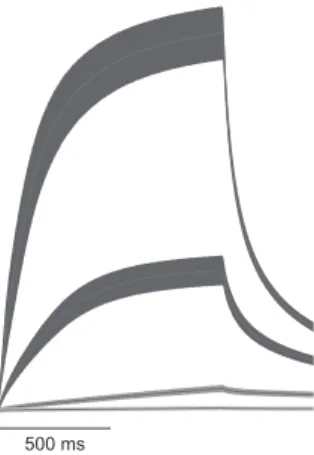
Figure 2.2 | PID signal for different odor concentrations
The PID signal was measured for the different concentrations of odorants used in the identification task. Error bars are mean ± SD (n = 400 traces). Scale bar: 500 ms. Each line corresponds to a different stimulus concentration (v/v): 10-1, 10-2, 10-3, 10-4, as indicated by color shading (highest concentration corresponding to the darkest shade). Stimulus onset (valve signal) corresponds in each case to the left-most edge of the trace.
For the experiments in Figs. 3.1-3.4, only mixtures with a total
odor concentration of 10-1 were used (Fig. 2.1a). For the
experiment in Fig. 3.5, we used the same mixture contrasts with
total concentrations ranging from 10-1 to 10-4 prepared using the
diluted odorants used for the identification task (Fig. 2.1d). In
each session, four different mixture pairs were pseudo-randomly
selected from the total set of 32 stimuli (8 contrasts at 4 different
total concentrations). Thus, for this task, a full data set comprised
4 individual sessions. For the experiments in Figs. 3.4a, b we
used two different sets of mixture ratios: 0/100, 17/83, 33.5/66.5,
50/50 in one experiment and 0/100, 39/61, 47.5/52.5, 49.5/50.5 in
the second experiment (Fig. 2.1c). In the experiment using 50/50
mixture ratios we used two filters both with the mixture 50/50,
one corresponding to the left-rewarded stimulus and the other one
to the right-rewarded stimulus. Thus, for the 50/50 mixtures, rats
were rewarded randomly, with equal probability for both sides.
2.4 Reaction time paradigm
The sequence and timing of task events is illustrated in Fig. 2.3.
Rats initiated a trial by entering the central odor-sampling port,
which triggered the delivery of an odor with delay (dodor) drawn
from a uniform distribution with a range of 300-600 ms. The odor
was available for up to 1 s after odor onset. Rats could exit from
the odor port at any time after odor valve opening, and make a
movement to either of the two reward ports. Trials in which the
rat left the odor sampling port before odor valve opening (4.2% of
trials) or before a minimum odor sampling time of 100 ms had
elapsed (1.1% of trials) were considered invalid. Odor delivery
was terminated as soon as the rat exited the odor port. Odor
sampling duration (OSD) was calculated as the difference
between odor valve actuation until odor port exit (Fig. 2.3b).
(Fig. 2.3 continues in the next page)
a
Odor Port Choice Port
Choice Port Trial start
Trial start Stimulus Choice Outcome
Correct
Error OH
Figure 2.3 | Two-alternative odor choice task
(a) Sequence of events in a behavioral trial, illustrated using a schematic of the ports and the position of the snout of the rat. (b) Illustration of the timing of events in a typical trial. Nose port photodiode and valve command signals are shown (thick lines). Measurements of odor sampling duration (OSD) and movement time (MT), as well as imposed delays (dodor, dwater and dinter-trial) are
indicated by arrows. Dashed lines indicate omitted time.
The stimulus onset delay (dodor) was drawn from a uniform
distribution between 300 and 600 ms, which creates a rising
hazard rate (i.e., the probability that an event is likely to occur,
given that it hasn’t occurred already), hence increasing stimulus
onset expectation during this period56,107. For comparison of low
and high stimulus-expectation, two groups of trials were selected,
an early onset, low stimulus-expectation condition, dodor =
300-400 ms, and a late onset, high stimulus-expectation condition,
dodor= 500-600 ms. Analysis of OSD and accuracy for these two
stimulus-expectation conditions were performed by conditioning
OSD and accuracy on these two different time periods of dodor.
The CV was calculated as the ratio of the SD to the mean of OSD.
Movement time (MT) was defined as the difference between odor
port exit and choice port entry time. For correct trials, water was
delivered from gravity-fed reservoirs regulated by solenoid valves
after the rat entered the choice port, with a delay (dwater) drawn
Odor Port
Odor Valve
Choice Port
Water Valve d
odor OSD MT
d
from a uniform distribution with a range of [0.1, 0.3] s. Reward
was available for correct choices for up to 4 s after the rat left the
odor sampling port. Trials in which the rat failed to respond to
one of the two choice ports within the reward availability period
(0.5% of trials) were also considered invalid. Reward amount
(wrew), determined by valve opening duration, was set to 0.024 ml
and calibrated regularly. A new trial was initiated when the rat
entered odor port, as long as a minimum interval (dinter-trial), of 4 s
from water delivery, had elapsed. Error choices resulted in water
omission and a “time-out” penalty of 4 s added to dinter-trial.
Behavioral accuracy was defined as the number of correct choices
over the total number of correct and incorrect choices.
The influence of previous rewards on the choice function of the
rats was estimated by calculating the psychometric curve
conditional on the presence of a reward in the preceding trial for
each odor stimulus (odor A or odor B).
Choice bias was calculated as the difference between left
(“A-side”) and right (“B-(“A-side”) choices divided by the total number of
choices, averaged across all trials. This measures the overall
tendency of the rats to go left (Choice bias> 0) or right (Choice
bias < 0). The influence of reward and difficulty of previous stimuli on choice bias was estimated by calculating the choice
bias for each current stimulus difficulty conditional on the
previous reward and stimulus difficulty.
The three types of invalid trials (in total 5.8 ± 0.8% of trials, mean