The role of posterior parietal cortex in multisensory decision-making

(1)

David Nunes Raposo

Dissertation presented to obtain

the Ph.D degree in Biology - Neuroscience

Instituto de Tecnologia Química e Biológica António Xavier | Universidade Nova de Lisboa

Oeiras,

(2)

David Nunes Raposo

Dissertation presented to obtain

the Ph.D degree in Biology - Neuroscience

Instituto de Tecnologia Química e Biológica António Xavier | Universidade Nova de Lisboa

Oeiras, November 2015

The role of posterior parietal cortex in

multisensory decision-making

(3)

(4)

Acknowledgements

The work presented in this thesis would not have been possible without the help of my colleagues and friends. First, I would like to thank Haley Zamer for helping me set up the lab’s first behavioral rigs and conduct the first behavioral experiments with humans and rodents. Petr Znamen-skiy and Santiago Jaramillo provided crucial advice on the design of the behavioral experiments, surgical procedures and electrophysiology. A big thanks to Barry Burbach for all the technical knowledge that he shared with me and his devoted assistance. I want to thank John Sheppard, Michael Ryan, Angela Licata and Amanda Brown, for their dedication and close collaboration on many of the experiments that I worked on. Matt Kaufman’s analytical thinking and ingenuity are an inspiration to me. I wish to thank him for his invaluable input and collaboration on this project. There are also my classmates and friends, Pedro Garcia da Silva and Diogo Peixoto, who were always available when I needed to discuss any scientific or personal issue. I thank them and wish them the best success for their future endeavors.

I also want to thank the members of my thesis committee, Zach Mainen and Megan Carey, for all the comments and suggestions on my work throughout the PhD. A special thanks to Rui Costa, my co-advisor, for being incomparably enthusiastic and supportive. He, more than I, always believed in my success. Most importantly, I would like to thank my su-pervisor, Anne Churchland, for daring to accept me as her first student despite my limited experience at the time, for her patience and guidance. I am very fortunate to have her as a mentor and friend.

(5)

Contributions

Haley Zamer, John Sheppard and Amanda Brown collaborated on the be-havioral experiments with humans and rats. John Sheppard was the lead researcher on the cue weighting experiments. Matt Kaufman collaborated on the analysis of electrophysiological data. He developed the PAIRS and Variance Alignment analyses. Michael Ryan, John Sheppard and Angela Licata collaborated on the optogenetic experiments. Anne Churchland contributed to all stages of the research, including the experimental de-sign and the writing of the manuscripts reporting the results presented here.

(6)

List of figures

1.1 Drift diffusion model . . . 6

2.1 Schematic of rate discrimination decision task and experimental setup 19

2.2 Subjects’ performance is better on multisensory trials . . . 22

2.3 Subjects make decisions according to event rates, not event counts . . 24

2.4 The multisensory enhancement is still present for the independent

con-dition . . . 27

2.5 Human subjects’ performance is better on multisensory trials even

when the synchronous and independent conditions are presented in

alternating blocks . . . 29

2.6 Subjects’ decisions reflect evidence accumulated over the course of the

trial . . . 31

2.7 Single sensory performance on rate discrimination task depends on

sensory reliability . . . 33

2.8 Subjects weigh auditory and visual evidence in proportion to sensory

reliability . . . 35

2.9 Reliability-based sensory weighting is observed consistently across

sub-jects . . . 38

3.1 Rats’ behavior in the rate discrimination task . . . 49

(10)

3.3 DREADDs expression and hystology . . . 52

3.4 Effect of PPC inactivation on use of evidence. . . 53

3.5 PPC neurons show mixed selectivity for choice and modality . . . 55

3.6 Choice preference/divergence are stronger on multisensory trials and

easy unisensory trials . . . 56

3.7 Choice preference is strongly correlated between auditory, visual and

multisensory trials . . . 57

3.8 Neural responses defy categorization . . . 59

3.9 Time-varying firing rate patterns across neurons . . . 61

3.10 Choice and modality can be decoded from population activity . . . . 62

3.11 Choice can be estimated on multisensory trials, even when the decoder

is trained on data from unisensory trials . . . 64

3.12 Many PPC neurons switch preference between decision formation and

movement . . . 66

3.13 PPC neurons exhibit different covariance patterns during decision

for-mation and movement . . . 68

4.1 Optical stimulation of PPC neurons disrupts visual decision-making . 76

4.2 Performance is unchanged during optical stimulation if PPC neurons

do not express ChR2 . . . 77

4.3 Probabilistic model fits rats’ behavioral data well . . . 79

4.4 Optical stimulation in PPC reduces influence of sensory evidence in

decisions . . . 80

4.5 Stimulation has a greater impact on decisions when it occurs early in

decision formation . . . 82

4.6 Optical stimulation reduces influence of visual evidence in choices

(11)

1 Introduction

Making a decision consists of committing to a plan of action, usually selected between

two or more competing alternatives. Numerous fields have studied the processes

in-volved in decision-making including psychology, economics, philosophy and statistics,

to name only a few. In neuroscience the study of decision-making has been extremely

fruitful in recent years and has focused on two main aspects: (1) perceptual

decision-making, interested in understanding how external information is perceived by the

sensory systems and used to make decisions; (2) value based decision-making,

in-terested in the mechanisms that cause and result from the association of subjective

values to the possible outcomes of a decision.

An important feature of decisions is that they can be made on very different and

flexible time scales. For example, we can make an immediate decision to stop the car

as we drive and see a red light in front of us. But we can also take a longer time to

make more complex decisions, such as deciding which career we want to pursue. This

characteristic of decision-making depends on the ability that animals have to combine

information over time and may be, in general, a hallmark of cognition (Shadlen and

Kiani, 2013).

In this thesis we aim at revealing some of the neural computations involved in

perceptual decisions that occur over time and are informed by the auditory and visual

sensory systems. The following sections will review our current understanding of the

(12)

time and across modalities.

1.1 Perceptual decision-making

In a simplified context of decision-making, a subject is given two alternative choices

and has to commit to one of them based on information provided by the external

world. Faced with this problem the brain must implement at least three

transfor-mation steps (Graham, 1989) from the moment when the sensory inputs arrive until

the moment the choice is made. First, it must transform the sensory input into a

higher-order representation that is informative for the decision (sensory evidence).

For example, when deciding which of two rectangles is wider, our brain needs to have

access to a representation of the width of the two rectangles to be able to compare

them. Second, it must use this representation of the input to select the most

appropri-ate response. This step can also be viewed as computing a “decision variable” or, in

other words, the probability of choosing one of the two alternative responses. Third,

it must implement the action associated with the appropriate choice, by

instantiat-ing the probabilistic representation into a discrete behavioral output (for review, see

Sugrue et al., 2005).

These transformations have been explored extensively in the primate visual and

oculomotor systems. In these studies monkeys were typically asked to discriminate

noisy visual stimuli and report their perceptual judgments using eye movements.

Primary and secondary visual areas of the cortex (V1 and V2) and higher visual

areas, such as V4 and middle temporal area (MT, also known as V5), were found to

play a critical role in the representation of sensory evidence. For example, neurons in

area MT respond to the direction of visual motion. On the other hand, areas in the

frontal and parietal cortices — e.g. lateral intraparietal area (LIP), frontal eye fields

(FEF) and supplementary eye field (SEF) — intermediate between sensory areas and

the oculomotor nuclei in the brainstem, are thought to be responsible for translating

(13)

1.1.1 Motion discrimination task

The random-dot motion direction discrimination task is, perhaps, the most successful

paradigm used in the study of perceptual decisions. It relies on the presentation of

dots that appear randomly on a circumscribed area of a screen (_∼ 5–10 ) which

is positioned in front of the subject. Some of these dots move towards one of two

possible predefined directions. The goal of the subjects is to report which direction

the dots are moving towards, usually by making an eye movement (saccade) into

one of two targets on the screen. This task is designed in such a way that allows

the experimenter to change the difficulty of each trial by varying the percentage of

coherently moving dots.

Variants of this paradigm have been used in multiple studies to show that neurons

in the cortical visual area MT carry signals that can be used by the subjects to

discriminate the direction of visual motion. Here we list some of the findings:

1. The majority of neurons in area MT are tuned to the direction of visual motion

(Albright et al., 1984);

2. The response of individual MT neurons correlates with behavioral accuracy /

psychophysical performance (Britten et al., 1992; Shadlen et al., 1996);

3. The firing rate of single neurons in MT significantly predicts the subjects’

choices, even on error trials, on a trial by trial basis (choice probability, Britten

et al., 1996);

4. Lesioning MT causes an impairment in subjects’ ability to discriminate the

direction of visual motion (Newsome and Par´e, 1988), suggesting the area is

necessary for the task;

5. Microstimulation of MT, taking advantage of the anatomical organization of the

area in terms of motion direction tuning, indicated that this area has a causal

(14)

These experiements not only showed the importance of MT in motion

discrimi-nation, they also led to new hypotheses. Britten, Newsome and colleagues suggested

that, in this task, the brain makes a decision based on the comparison between the

firing rate of two pools of neurons, each of them most sensitive to one of the two

possible directions of motion (Newsome et al., 1989; Britten et al., 1992). As an

ex-ample, if on a particular trial the random dots move leftwards, a pool of neurons with

a “preference” for motion towards the left (more tuned to that direction of motion)

would on average fire more than a pool of neurons with a preference for motion in

the opposite direction (rightward motion). The difference between the firing rates of

these two pools of neurons can be used as a decision variable — if the difference is

positive (on average), choose ‘left’; if the difference is negative, choose ‘right’.

In the case of a weak stimulus (low proportion of coherently moving dots) the

difference between the firing rate of the two pools of neurons becomes close to zero.

This compels the subjects to take some time before committing to a particular choice.

In other words, the subjects need to accumulate evidence for a certain period of time

in order to make accurate decisions. This corresponds to allowing the decision variable

to be integrated over time, as more evidence arrives, until it is possible to determine

with confidence if its value is positive or negative.

Together, these studies established a new paradigm for investigating the neural

mechanisms of decision formation by making it possible to characterize neural

re-sponses as the decision process unfolds.

One other key aspect of this task is that it sets up a clear association between

a decision about a stimulus and a behavioral response to report that decision: a

saccade towards one of two targets. This allowed scientist to look for a signature of

the decision variable in particular brain areas involved in the guiding or planning of

eye movements, like the lateral intraparietal area (LIP), the superior colliculus (SC)

(15)

1.1.2 Drift di

ff

usion model

Decisions that are based on noisy, unreliable information may benefit from the process

of integrating that same information over time. The reason is that integration provides

a way to average out the noise and therefore achieve more accurate decisions. This

is the idea behind integration models such as thedrift diffusion model (DDM). The

DDM assumes that infinitesimally small samples of a noisy signal are added together

continuously and that this summation represents evidence accumulated over time.

When this accumulated evidence reaches an upper or a lower bound, an appropriate

response is triggered (Ratcliff, 1978).

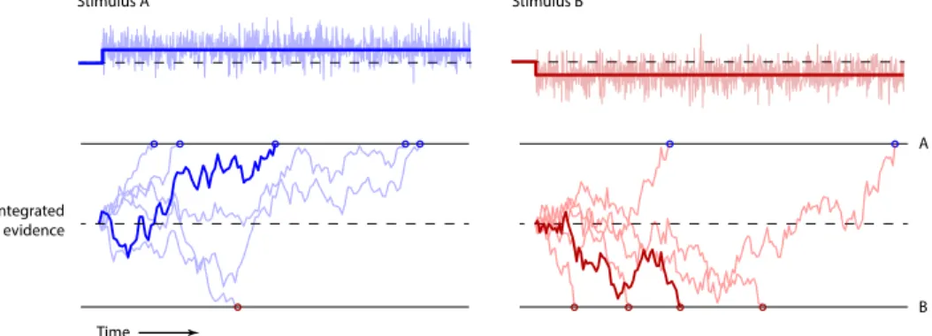
To be more specific, let’s assume that a “decision system” implementing the DDM

receives an input signal corrupted by gaussian noise (stimulus), with mean µ and

standard deviationσ (Figure 1.1, top). This device will sum this stochastic stimulus

over time (integrated evidence), producing a drift that fluctuates over time (Figure

1.1, bottom). At some point this drifting integrated evidence will cross one of two

thresholds — A or B (upper or lower bound). This event triggers the response of

the system: if threshold A was crossed, the systems returns the response RA (e.g.

select target ‘A’); if threshold B was crossed, the system returns the response RB

(e.g. select target ‘B’).

In the context of the motion discrimination task, the parameter µis defined by

the stimulus strength (motion coherence) and the noise parameter σ is considered

constant. The distance between the decision boundaries A and B and the initial value

of integrated evidence (evidence = 0) depends on the response bias of the subject, as

measured by the point of subjective equality (PSE) of the psychometric curve (see

Methods for explanation on psychometric curves).

This is a very simple model that, nonetheless, fits the behavioral data remarkably

well (Palmer et al., 2005). Furthermore, neurophysiological data collected from

sub-jects performing the task come in support of this view of integration of evidence at

(16)

Integrated evidence

Stimulus A

A

B Stimulus B

Time

Figure 1.1: Drift diffusion model. Adapted from Uchida et al. (2006). Top,

schematic of two example input signals (saturated blue/red line) and signal with added gaussian noise (stimulus; faded ragged blue/red trace). Bottom, cumulative sum of six instantiations of the two example stimuli (representing the integrated evidence), in which the signal was kept constant and the added noise varied. The noise makes the integrated evidence drift over time. At some point in time this integrated evidence crosses one of two thresholds (A or B), which is indicated by the blue/red circles.

1.1.3 A signature of the decision variable

The lateral intraparietal area (LIP) is a subregion of the posterior parietal cortex

(PPC). It receives inputs from visual areas such as V3, V4 and MT (Felleman and

Van Essen, 1991) and the pulvinar (Hardy and Lynch, 1992). Neurons in this area

encode the direction and amplitude of an intended saccade (Gnadt and Andersen,

1988) and send these signals to structures involved in the control of eye movements

(Andersen et al., 1990). Researchers soon hypothesized that the activity of LIP

neurons could be correlated with a decision variable.

Indeed, experiments using the motion discrimination task described above revealed

that some neurons in LIP reflect the accumulation of evidence in favor of one choice

versus the other, i.e., the integration of the difference in firing between the two pools

of MT neurons (Shadlen and Newsome, 1996). Moreover, the firing rate of these

LIP neurons increased proportionally to the motion coherence and reached the same

singular value, across trials, just before the decision was reported (Roitman and

(17)

a specific threshold — or level of confidence in the decision — is crossed, very much

consistent with the drift diffusion model.

Although microstimulation of LIP neurons during motion discrimination produces

a contralateral response bias (Hanks et al., 2006), this effect is much smaller compared

to the one observed from microstimulation of MT neurons. It was not yet established if

LIP is, indeed, necessary for motion discrimination or if, instead, evidence integration

occurs elsewhere and this computation is simply reflected in LIP. One the reasons why

it has been difficult to state the importance of LIP in the motion discrimination task

relates to the absence of techniques that would allow stimulation or inactivation of the

specific outputs of MT that connect to LIP. Optogenetics opens up this possibility but

methods for using this technique in primates are still in an early stage of development.

1.2 Integrating multiple sensory modalities

In the previous section we discussed how integration over time can ameliorate the

problem of making decisions based on noisy and unreliable evidence. In the current

section we will examine how the use of more than one sensory modality benefits

decision-making under the same conditions.

Our observation of the world may sometimes lead to ambiguous or uncertain

judgments. For example, imagine a situation where we are sitting inside an immobile

train at the station and there is a second train, also immobile, next to ours. If that

second train slowly starts moving, we sometimes perceive as if the train we are on is

the one moving instead. This illusion happens because this is an ambiguous visual

scene — based on our visual system, either scenario (‘my train is moving’ versus

‘the other train is moving’) would be conceivable. In situations like this one our

judgment typically improves when we use another sensory modality to disambiguate

our perception of the scene. In this case, using our vestibular system, for example,

would help us to recognize that we are not moving.

Many studies have approached this question of how the brain combines multiple

(18)

therefore, be able to make more accurate decisions. Here we will introduce some of

the current views about multisensory integration.

1.2.1 Cue combination framework

The word ‘cue’ refers to a piece of sensory information that gives rise to a sensory

estimate of a particular scene. The process of combining different cues is referred to

as “cue combination” (or “cue integration”).

If we try to estimate the precise location of a bird that hides behind the leaves of a

tree, we may use both our vision and our audition, if the bird is singing, to do so. Our

perception of the location of the bird must then be given by a mixture between our

visual and auditory perceptions. But how exactly does the brain combine the two?

One possibility is that the brain computes a separate estimate for each cue (visual

cue and auditory cue) and then combines these estimates by computing a weighted

average of the two, creating a final estimate (Clark and Yuille, 1990).

The maximum likelihood estimation framework provides an ‘optimal’, i.e. most

advantageous, solution to the problem of determining how heavily each of the

indi-vidual estimates should be weighted to compute the final estimate. Assuming that

the noise corrupting each individual estimate is independent and gaussian, the best

final estimate is the one that weighs each estimate by the inverse of their variances

— maximum likelihood estimate, or MLE (see Methods for detailed deduction; for

review, see Ernst and B¨ulthoff, 2004). This ‘optimal’ way of integrating evidence

achieves a final estimate that is unbiased and that has the lowest possible variance.

From a Bayesian perspective, suppose that we want to estimate an external

vari-able,S, using two sensory cues. It is fair to assume that the neural representation of

these two cues,r1 andr2, is noisy and can, therefore, be seen as probabilistic. The

possible values ofS are then given by a probability density function,P(S|r1, r2). If

the noise affecting each cue is independent, P(S|r1, r2) can be calculated using the

Bayes’ theorem:

P(S|r1, r2) =

P(r1|S)P(r2|S)P(S) P(r1)P(r2)

(19)

The left hand side of this equation, called the posterior distribution, can be used to

estimate S (by taking the mean of this distribution, for example) and includes the

uncertainty associated with that estimate (its variance). P(r1|S) and P(r2|S) are

called thelikelihood functions and quantify the probability of observing a particular

neural response for each of the two cues. P(S), theprior distribution, represents the

probability of a particular eventSoccurring in the first place. Here, our goal is to find

the value ofSthat maximizes theposterior. This optimization process is independent

of the termsP(r1) andP(r2). Assuming gaussian likelihoods and a uniform prior, it

follows that the solutionS with the smallest variance is the MLE (Knill and Pouget,

2004; Angelaki et al., 2009).

Many studies have shown that this model describes well the behavior of human

subjects in cue combination tasks. In a target localization task, humans combine

au-ditory and visual cues, in an optimal way, according to each cue’s reliability (Battaglia

et al., 2003; Alais and Burr, 2004; Ghahramani and Wolpert, 1997). Humans

com-bine visual and haptic cues to optimally estimate object size (Ernst and Banks, 2002).

Surface slant estimates by humans using depth and texture cues result from optimal

cue combination (Knill and Saunders, 2003).

Most multisensory integration studies, like the ones mentioned above, have relied

on careful behavior and psychophysics with human subjects. Only a few recent studies

have gone further and approached this problem with a combination of phychophysics

and neural recordings in non-human primates, in search for a signature of multisensory

integration in the brain.

1.2.2 Heading discrimination task

Gu, Angelaki and colleagues designed a two-alternative forced choice task that asked

subjects to judge their heading direction using visual and vestibular cues. In this

task, subjects (macaque monkeys) were seated on a platform that moved on the

horizontal plane. A projector attached to the platform displayed a three-dimensional

field of moving dots that provided optic flow on a given direction. For a subject

(20)

the opposite direction of flow. In each trial, the subjects experienced forward motion

with a small leftward or rightward component and were asked to report the perceived

heading direction. They found that subjects performed significantly better when

they used both cues (multisensory condition), compared to when they used only one

(single sensory condition). Subjects’ choices and how much they improved were well

predicted by the maximum likelihood model described above. Moreover, when the

reliability of the visual and vestibular cues changed, subjects quickly adjusted the

relative weighting of two cues as the model predicted (Gu et al., 2008).

Many neurons in the dorsal medial superior temporal area (MSTd) had been

found to respond strongly to both optic flow and translational movement (Duffy,

1998), making this area a good candidate in the search for a signature of heading

perception. In a subset of neurons that had the same heading preference with both

visual and vestibular cues (“congruent neurons”), heading tuning became steeper —

more sensitive — in the multisensory condition. This finding suggested that these

neurons could be involved in heading discrimination. Furthermore, choice probability

analysis showed that trial-to-trial fluctuations in the firing rate of “congruent neurons”

was strongly correlated with the fluctuations in the subjects’ perceptual decisions,

consistent with the hypothesis that monkeys monitored these neurons to perform the

task.

Together these studies established the foundation for future research on the neural

basis of multisensory decisions and opened doors to new models of sensory integration.

1.2.3 Models of multisensory integration

One of the main findings in the studies mentioned above was that cue weighting was

adjusted on-the-fly as the reliability of each cue was changed by the experimenter

from trial to trial. This revelation suggests that optimal integration, which requires

knowledge of the variance of the estimates, can be accomplished on-line, as the

evi-dence arrives and allows us to exclude particular neural models of sensory integration.

Models that rely on plasticity to compute the uncertainty associated with a

(21)

cue weighting. Instead, the neural implementation of cue combination may, perhaps,

be depended on network dynamics.

A plausible mechanism for determining the variance of a sensory estimate on-line

is one that monitors the different responses of a population of neurons to a single

sensory cue — referred to, in the literature, as a population code. As an example,

consider a population of neurons in primary auditory cortex that are sensitive to tone

frequency. This means that each neuron will fire the most in response to its preferred

tone and will fire less as the frequency of the tone diverges away from its preferred

one (tunning) In response to a particular tone, the firing of a population of auditory

neurons will follow a distribution that peaks at the presented tone frequency and with

a variance proportional to the uncertainty of the neural representation of the stimulus.

Moreover, combining the activity of two such populations of neurons, by multiplying

the two population firing distributions, results in an overall response distribution that

corresponds to the solution provided by maximum likelihood estimation (Ernst and

B¨ulthoff, 2004). In a Bayesian context, this corresponds to multiplying the likelihood

functions to obtain the posterior distribution (assuming a flat prior). This is true not

only for two populations of neurons that respond to only one sensory modality (e.g.

two populations of auditory neurons), but also for two populations of neurons that

respond to different sensory modalities — e.g. a population of auditory neurons and

a population of visual neurons.

Many studies have proposed neural models of sensory integration using

popula-tions codes (Pouget et al., 2000; Zemel and Dayan, 1997). Ma, Pouget and colleagues

demonstrated that, by taking advantage of the probabilistic nature of neural firing

— assuming Poisson-like variability — cue combination could be implemented as a

simple linear combinations of populations of neural activity (Ma et al., 2006).

How-ever, their model assumes fixed cue weighting and, thus, fails to explain the impact

of cue reliability in the combination rule (Morgan et al., 2008).

Ohshiro and colleagues proposed that “divisive normalization” could explain many

of the features of multisensory integration, including the change in neural weights

(22)

one auditory neuron and one visual neuron) with overlapping receptive fields provide

input to the same multisensory neuron. In summary, the activity of each multisensory

neuron depends on a linear combination of the inputs, followed by an expansive

power-law nonlinearity, and is divided by the net activity of all multisensory neurons.

“Divisive normalization” (Heeger, 1992) has been used to explain how neurons

in primary visual cortex respond to a combination of stimuli with different contrasts

and orientations (Carandini et al., 1997) and proposed to be involved in attention

modulation (Reynolds and Heeger, 2009). It may, therefore, be a prevalent cortical

computation that relies on relatively simple operations, making it a plausible model

of multisensory integration.

1.3 The posterior parietal cortex

The posterior parietal cortex (PPC) is an association area of the brain traditionally

seen as critical for visuo-spatial perception and spatial attention. However, in recent

years, multiple studies have proposed its involvement in a wide range of cognitive

functions, such as working memory and decision-making.

In primates, the PPC receives inputs from the pulvinar and lateral posterior nuclei

of the thalamus. It is extensively connected with multiple sensory areas — visual,

auditory, somatosensory and vestibular sensory systems (Avillac et al., 2005) and

with subcortical structures, such as the superior colliculus (SC) and striatum. PPC

is also strongly interconnected with the prefrontal cortex (PFC), traditionally

asso-ciated with higher cognitive operations and executive functions (Miller and Cohen,

2001), premotor cortex and frontal eye fields (FEF). Its anatomical characteristics

have led researchers to propose that PPC is involved in directed spatial attention.

Indeed, unilateral and bilateral lesioning of PPC in humans cause strong deficits in

attentional processing, such as the notorious hemispatial neglect (for review, see Reep

and Corwin, 2009). Situated between multiple sensory inputs and a motor output,

PPC is also in a privileged position for the computation of the variables necessary

(23)

re-flect, for example, evidence accumulation (see Section 1.1.3), categorization of visual

stimuli (Freedman and Assad, 2006), estimation of numerical quantities (Nieder and

Miller, 2004) and reward expectation (Platt and Glimcher, 1999). These studies show

a remarkable correlation between the neural activity in PPC and the decisions the

subjects were asked to make. However, it is not yet known whether PPC neurons

simply reflect a neural correlate of these decision-related signals or whether they are

indeed responsible for the computations of these signals. If the latter is true, it would

require downstream areas to be able to de-multiplex — i.e., independently decode —

the different signals carried by PPC neurons (Huk and Meister, 2012).

In rodents, the existence of a PPC has only recently been established, with several

studies identifying PPC as an autonomous region of the rodent brain (Kolb and Tees,

1990). In studies using retrograde tracers, Chandler, Reep and colleagues have found

that PPC in rodents could be defined based on its afferents from the lateral dorsal

and lateral posterior nuclei of the thalamus (Chandler et al., 1992; Reep et al., 1994).

Unilateral lesioning of this brain area in rodents produces severe multimodal neglect

— visual, tactile and auditory — similar to that observed in humans (Corwin et al.,

1994; King and Corwin, 1993). However, it is not yet clear the degree to which

the rodent PPC is homologous to the primate PPC. Other studies have shown the

importance of PPC in spatial attention as well as in learning (Robinson and Bucci,

2012) and memory (Myskiw and Izquierdo, 2012) in rodents, but its importance in

perceptual decisions has not been established in this model system.

1.4 Mixed selectivity and the argument against

neural categories

Neurons in early sensory areas typically (although not exclusively; see Saleem et al.,

2013) respond to a particular feature of the sensory environment. For example, some

neurons in primary visual cortex are active when a moving bar with a specific

orien-tation crosses the neuron’s receptive field. In contrast, neurons in higher order brain

(24)

feature of the task the organism is dealing with. This ability that neurons in some

brain areas have to respond to multiple features is called “mixed selectivity”. The

PFC is predominantly composed of neurons with mixed selectivity. This makes its

responses very heterogeneous and, therefore, difficult to interpret. However, mixed

selectivity might be crucial in giving areas like PFC the ability to be involved in

multiple tasks. Rigotti, Fusi and colleagues have shown that, whilst neurons in PFC

encode distributed information about many task-relevant features, each of those

fea-tures could be easily decoded from this population ofmixed-selective neurons. They

argue that mixed selectivity is a signature of high-dimensional neural representations.

This high-dimensionality is what allows a linear classifier — such as a simple

neu-ron model that combines information from a population of neuneu-rons — to decode

information about any task-relavant feature (Rigotti et al., 2013).

Recent studies have extended mixed selectivity to neurons in PPC. Monkey LIP

neurons were found to frequently respond to a mixture of decision signals, such as the

accumulated evidence, and decision-irrelevant signals — other parameters of the task

that do not inform the decision process, such as the presence of a choice target in

the neurons receptive field (Meister et al., 2013). Other studies have emphasized this

property of LIP neurons by showing that, while these neurons are strongly influenced

by visual-spatial factors, such as the direction of a future saccade, they also carry

signals about more abstract, nonspatial factors, such as the learned category of the

direction of moving dots (Freedman and Assad, 2009).

Here we argue that the view that individual neurons belong to specialized classes,

apt for particular computations, while important for understanding early sensory

ar-eas, may be inappropriate for the study of higher order brain areas. Instead, we

speculate that single neurons in areas such as PPC and PFC may reflect a random

combination of task-related parameters, therefore challenging the idea of neural

cat-egories. Mixed selectivity does not imply random combination of parameters per se.

However, there is a major advantage to this kind of configuration: a task

parame-ter that is randomly distributed across a population of neurons can be decoded by

(25)

see Ganguli and Sompolinsky, 2012). An important consequence of this is that if a

population with these characteristics is randomly connected to multiple downstream

neurons, each of these neurons would receive enough information to be able to read

out (decode) any particular task parameter that is encoded by the neural population.

1.5 Thesis outline

The following chapters report the main findings that came out of this research work

(Chapters 2–4), the methodologies and details of the analyses used (Chapter 5) and,

lastly, a summary of the conclusions we take and their relevance in the larger picture

of understanding the computations that allow multisensory decision-making to take

place in the brain (Chapter 6).

Chapter 2 describes our efforts to bring the rodent model to the field of

mul-tisensory decision-making. We lay out a new task that allowed us to observe that

rodents, as humans, are able to combine auditory and visual information to make

more accurate decisions.

In Chapter 3 we reveal the response properties of neurons in the posterior parietal

cortex of rats performing a multisensory decision-making task. The neural recordings

that we have conducted reveal mixed selectivity of PPC neurons and suggest that the

population is category-free — characteristics that allow them to encode multiple task

parameters, while granting easy decoding of those same parameters by downstream

neurons. In this chapter we also analyze the impact of PPC inactivation during

multisensory decision-making.

Chapter 4 describes the consequences of disrupting the normal activity of PPC in

a spatially and temporally precise manner, using optogenetics. Our findings suggest

that disruption impairs the use of sensory evidence in decisions and is followed by a

(26)

2 Multisensory decision-making in

rats and humans

A large body of work has shown that animals and humans are able to combine

infor-mation across time to make decisions in some circumstances (Roitman and Shadlen,

2002; Mazurek et al., 2003; Palmer et al., 2005; Kiani et al., 2008). Specifically,

combining information across time can be a good strategy for generating accurate

de-cisions when incoming signals are noisy and unreliable (Link and Heath, 1975; Gold

and Shadlen, 2007). For noisy and unreliable signals, combining evidence across

sen-sory modalities might likewise improve decision accuracy, but little is known about

whether the framework for understanding combining information over time might

extend to combining information across sensory modalities.

The ability of humans to combine multisensory information to improve perceptual

judgments for static information has been well established (for review, see Alais et al.,

2010). Psychophysical studies have shown that multisensory enhancement requires

that information from the two modalities be presented within a temporal “window”

(Slutsky and Recanzone, 2001; Miller and D’Esposito, 2005). Physiological studies

suggest the same: SC neurons show enhanced responses for multisensory stimuli

only when those stimuli occur close together in time (Meredith et al., 1987). Such a

temporally precise mechanism would serve a useful purpose for localizing or detecting

objects. Therefore, temporal synchrony (or near-synchrony) provides an important

(27)

Burr et al., 2009).

In other circumstances, multisensory decisions might have more lax requirements

for the relative timing of events in each modality. For example, when multiple

audi-tory and visual events arrive in a continuous stream, temporal synchrony of individual

events might be difficult to assess. Auditory and visual stimuli drive neurons with

different latencies (Pfingst and O’Connor, 1981; Maunsell and Gibson, 1992;

Recan-zone et al., 2000), making it difficult to determine which events belong together.

It is not known whether information in streams of auditory and visual events can

be combined to improve perceptual judgments; if they can, this could be evidence

for a different mechanism of multisensory integration that has less strict temporal

requirements compared with the classic, synchrony-dependent mechanisms.

To invite subjects to combine information across both time and sensory

modal-ities for decisions, we designed an audiovisual rate discrimination decision task. In

the task, subjects are presented with a series of auditory and/or visual events and

report whether they perceive the event rates to be high or low. Because of differing

latencies for the auditory and visual systems, our stimulus would pose a challenge to

synchrony-dependent mechanisms of multisensory processing. Nevertheless, we saw

a pronounced multisensory enhancement in both humans and rats. Importantly, this

enhancement was present whether the event streams were identical and played

syn-chronously or were independently generated, suggesting that the enhancement did

not rely on mechanisms that require precise timing. Together, these results suggest

that some mechanisms of multisensory enhancement might exploit abstract

informa-tion that is accumulated over the trial durainforma-tion and therefore must rely on neural

circuitry that does not require precise timing of auditory and visual events.

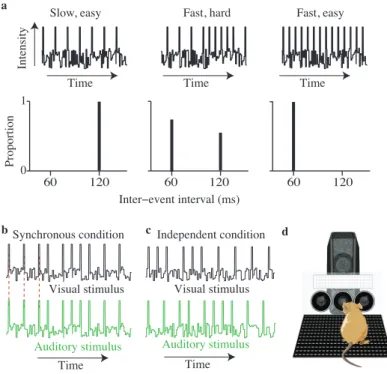
2.1 Rate discrimination task

We developed a novel behavioral task designed to invite subjects to combine

informa-tion across time and sensory modalities. Each trial consisted of a series of auditory

(28)

noise between events (Figure 2.1a, top). Visual events were flashes of light, and

audi-tory events were brief sounds (see below for methodological details particular to each

species). The amplitude of the events was adjusted for each subject so that on the

single-sensory trials performance was_∼70–80% correct and matched for audition and

vision. We chose these values because previous studies have indicated that

multisen-sory enhancement is the largest when individual stimuli are weak (Stanford et al.,

2005). This appears to be particularly true for synchrony-dependent mechanisms of

multisensory integration (Meredith et al., 1987).

Trials were generated so that the instantaneous event rate fluctuated over the

course of the trial. Each trial was created by sequentially selecting one of two

in-terevent intervals: either a long duration or a short duration (Figure 2.1a, bottom)

until the total trial duration exceeded 1000 ms (or occasionally slightly longer/shorter

durations for “catch trials”; see below). Trial difficulty was determined by the

propor-tion of interevent intervals from each durapropor-tion. As the proporpropor-tion of short intervals

varied from zero to one, the average rate smoothly changed from clearly low to clearly

high. For example, when all of the interevent intervals were long, the average rate was

clearly low (Figure 2.1a, left), and similarly when all of the interevent intervals were

taken from the short interval, the average rate was clearly high (Figure 2.1a, right).

When interevent intervals were taken more evenly from the two values, the average

of the fluctuating rate was intermediate between the two (Figure 2.1a, center). When

the number of long intervals exceeded the number of short intervals, subjects were

rewarded for making a “low rate” choice and vice versa. When the numbers of short

and long intervals in a trial were equal, subjects were rewarded randomly. Note that

in terms of average rate this reward scheme places the low rate–high rate category

boundary closer to the lower extreme (all long durations) than to the higher extreme

(all short durations) because of the differing duration of the intervals. The strategies

of both human and rat subjects reflected this: typically, subjects’ points of subjective

equality (PSEs) were closer to the lowest rate and less than the median of the set

of unique stimulus rates presented. Nevertheless, for simplicity, we plotted subjects’

(29)

0 500 1000 0 0.5 1 1.5 2

0 500 1000

0

0.5 1 1.5 2

0 500 1000

0 0.5 1 1.5 2 Proportion Fast, easy Fast, hard 0 1 60 120

Inter−event interval (ms) Slow, easy

60 120 60 120

Time Time Time Intensity b c a d

Synchronous condition Independent condition

Auditory stimulus

Visual stimulus

Auditory stimulus

Visual stimulus

Time Time

Figure 2.1: Schematic of rate discrimination decision task and experimental

setup. a, Each trial consists of a stream of events (auditory or visual) separated by long or short intervals (top). Events are presented in the presence of ongoing white noise. For easy trials, all interevent intervals are either long (left) or short

(right). More difficult trials are generated by selecting interevent intervals of both

values (middle). Values of interevent intervals (bottom) reflect those used for all

human subjects. b,Example auditory and visual event streams for the synchronous

condition. Peaks represent auditory or visual events. Red dashed lines indicate that

auditory and visual events are simultaneous. c, Example auditory and visual event

streams for the independent condition. d, Schematic drawing of rodent in operant

conditioning apparatus. Circles are the “ports” where the animal pokes his nose to initiate stimuli or receive liquid rewards. The white rectangle is the panel of LEDs. The speaker is positioned behind the LEDs.

we analyzed subjects’ responses as a function of the number of short intervals in a

trial rather than stimulus rate.

For single-sensory trials, event streams were presented to just the auditory or

just the visual system. Visual trials were always 1000 ms long. Auditory trials were

usually 1000 ms long, but we sometimes included catch trials that were 800 or 1200 ms.

(30)

was to determine whether subjects’ decisions were based on just event counts or

event counts relative to the total duration over which those counts occurred. Catch

trials constituted a total of 2.31% of the total trials. We reasoned that using such a

small percentage of the trials for variable durations would make it possible to probe

subjects’ strategy without encouraging them to alter it. For these trials, we rewarded

subjects based on event counts rather than the rate. This should have increased the

likelihood that subjects would have made their decisions based on count, if they were

able to detect that stimuli were sometimes of variable duration.

For multisensory trials, both auditory and visual stimuli were present and played

for 1000 ms. To distinguish possible strategies for improvement on multisensory trials,

we used two conditions. First, in the synchronous condition, identically timed event

streams were presented to the visual and auditory systems simultaneously (Figure

2.1b). Second, in the independent condition, auditory and visual event streams were

on average in support of the same decision (i.e., the proportion of interevent

inter-vals taken from each duration was the same), but each event stream was generated

independently (Figure 2.1c). As a result, auditory and visual events frequently did

not occur at the same time. Auditory and visual events did not occur simultaneously

even for the highest stimulus strengths because we imposed a 20 ms delay between

events. Although a 20 ms delay does prevent auditory and visual events from being

synchronous at the highest and lowest rates, the delay may be too brief to prevent

au-ditory and visual stimuli from being perceived as synchronous (Fujisaki and Nishida,

2005). To be sure that our conclusions about the independent condition were not

affected by these “perceptually synchronous” trials at the highest and lowest rates,

we analyzed the independent condition both with and without the easiest trials (see

Section 2.3). The multisensory effects we observed were very similar regardless of

whether or not we included the easy trials.

Because auditory and visual event streams were generated independently, trials

for this condition fell into one of four categories:

• Matched trials, where auditory and visual event streams had the same number

(31)

• Bonus trials, where both modalities provided evidence for the same choice, but

one modality provided evidence that was one events/s stronger than the other

(i.e., auditory and visual streams had proportions of short or long durations

both above or below 0.5, but were not equal);

• Neutral trials, where only one modality provided evidence for a particular

choice, whereas the other modality provided evidence that was so close to the

PSE that it did not support one choice or the other;

• Conflict trials, where each modality provided evidence for a different choice.

Conflict trials were used to reveal differential weighting of sensory cues by

explic-itly varying the reliability of the single-sensory stimuli (see Section 2.5), as previously

described in other multisensory paradigms (Fine and Jacobs, 1999; Hillis et al., 2004;

Fetsch et al., 2009).

2.2 Rats, as humans, combine auditory and

visual stimuli to improve decision accuracy

We examined whether subjects could combine information about the event rate of a

stimulus when the information was presented in two modalities. Combining evidence

should produce lower multisensory thresholds relative to single sensory thresholds.

We first describe results from the synchronous condition where the same stream of

events was presented to the auditory and visual systems, and the events occurred

simultaneously (Figure 2.1b).

We quantified subjects’ performance by computing their probabilities of

high-rate decisions across the range of trial event high-rates and fitting psychometric functions

to the choice data using standard psychophysical techniques (see Methods). Figure

2.2a shows results for the synchronous condition for a representative human subject:

the subject’s psychophysical threshold (σ) was lower for multisensory trials compared

with single-sensory trials (Figure 2.2a, blue line is steeper than green and black lines),

(32)

10 12 14 16 0 0.25 0.5 0.75 1

Rate (events • s−1)

b

8 10 12 14 0 0.25 0.5 0.75 1 a c Human Rat

Prop. high choices

1 2 3 4 5

1 2 3 4 5 Optimal threshold

Measured multisensory threshold

Figure 2.2: Subjects’ performance is better on multisensory trials. a,

Perfor-mance of a single subject plotted as the fraction of responses judged as high against the event rate. Green trace, auditory only; black trace, visual only; blue trace, multisensory. Error bars indicate SEM (binomial distribution). Smooth lines are

cu-mulative Gaussian functions fit via maximum-likelihood estimation. n= 7680 trials.

b, Same as a but for one rat (rat 3). n = 12459 trials. c, Scatter plot comparing

the observed thresholds on the multisensory condition with those predicted by the single-cue conditions for all subjects. Circles, human subjects; squares, rats. Green symbols are for the example rat and human shown in a and b. Black solid line shows

x = y; points above the line show a suboptimal improvement. Error bars indicate

95% CIs. Prop, Proportion.

difference between the single-sensory and multisensory thresholds was highly

signif-icant (auditory: p = 0.0001; visual: p < 0.0003); the change in threshold was not

significantly different from the optimal prediction (see ‘Optimal cue weighting’,

Equa-tion 5.4 in Methods for details; measured: 1.75 [1.562, 1.885]; predicted: 1.69 [1.54,

1.84]; p = 0.38). In contrast, the PSE for multisensory trials was similar to those

seen on single-sensory trials (auditory: p= 0.06; visual: p= 0.52).

The example was typical: all subjects we tested showed an improvement on the

multisensory condition, and this improvement was frequently close to optimal (Figure

2.2c, circles are close to thex=yline, indicating optimal performance). On average,

this improvement was not accompanied by a change in PSE (mean PSE difference

between visual and multisensory: 0.54 [0.48, 1.56], p = 0.23; mean PSE difference

between auditory and multisensory: 0.05 [₋0.66, 0.75],p= 0.87).

Significant multisensory enhancement was also observed in all three rats. Figure

2.2b shows results for a single rat. The difference in thresholds between the

single-sensory and the multisingle-sensory trials was highly significant (auditory: p <10 5

(33)

p <10 5

). The improvement exceeded that predicted by optimal cue combination

(measured: 1.97 [1.72, 2.21]; predicted: 2.70 [2.57, 2.83]; p < 10 5

). This

improve-ment was also seen in the remainder of our rat cohort (Figure 2.2c, squares); the

improvement was significantly greater than the optimal prediction in one of the two

additional animals (rat 1,p <10 5

); the improvement nearly reached significance in

a third (rat 2,p= 0.06).

Multisensory enhancement on our task could be driven by decisions based on

estimates of event rate of the stimulus or estimates of the number of events. Human

subjects have previously been shown to be adept at estimating counts of sequentially

presented events, even when they occur rapidly (Cordes et al., 2007). In principle,

either strategy could give rise to uncertain estimates in the single-sensory modalities

that could be improved with multisensory stimuli. To distinguish these possibilities,

we included a small number of random catch trials that were either longer or shorter

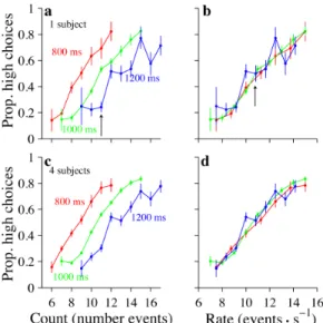
than the standard trial duration. Consider an example trial that has 11 events (Figure

2.3a, arrow). If subjects use a counting strategy, they would make the same proportion

of high choices whether the 11 events are played over 800, 1000, or 1200 ms. We did

not observe these results in our data. Rather, subjects made many fewer high choices

when the same number of events were played over a longer duration (Figure 2.3a,

blue trace) compared with a shorter duration (Figure 2.3a, red trace).

These findings argue that subjects normalize the total number of events by the

duration of the trial. In fact, the example subject in Figure 2.3, a and b, normalized

quite accurately: he made the same proportion of high choices for a given rate (Figure

2.3c, arrow) whether that rate consisted of a small number of events played over a

short duration (red traces) or a larger number of events played over a longer durations

(green and blue traces). The tendency to make choices based on stimulus rate rather

than stimulus count was evident when examined in a single subject (Figure 2.3a,b) and

in the population of four subjects (Figure 2.3c,d). Note that our subjects exhibited

such a rate strategy despite the fact that we rewarded them based on the absolute

(34)

Figure 2.3: Subjects make decisions according to event rates, not event counts. a, Example subject. Abscissa indicates the number of event counts. Each colored line shows the subject’s performance for trials where the event count on the abscissa was presented over the duration specified by the labels. For a given event count (11 events, black arrow) the subject’s choices differed depending on trial

duration. n= 3656 trials. b, Same data and color conventions as in a except that

the abscissa indicates event rate instead of count. For a given event rate (11 events/s,

black arrow), the subject’s choices were very similar for all trial durations. c, d,Data

for four subjects; conventions are the same as in a and b. n = 9727 trials. Prop,

Proportion.

2.3 Multisensory enhancement occurs even when

audio-visual events are asynchronous

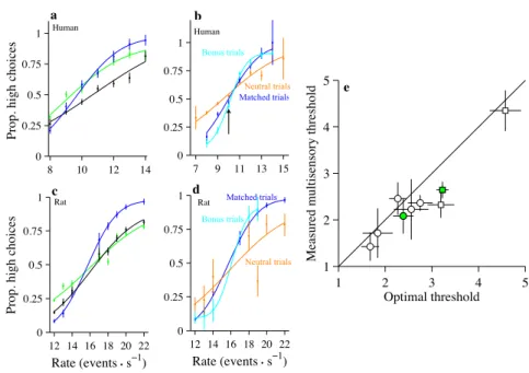
The multisensory enhancement observed for our task (Figure 2.2) might simply have

resulted because the auditory and visual stimuli were presented amid background

noise and therefore were difficult to detect. Thus, in the synchronous condition,

multisensory information may have enhanced subjects’ performance by increasing

the effective signal-to-noise ratio for each event by providing both auditory and visual

events at the same time. To evaluate this possibility, we tested subjects on a condition

(35)

achieved this by generating auditory and visual event streams independently. We

term this the “independent condition”. On each trial, we used the same ratio of short

to long events for the auditory and visual stimuli. First, we restricted our analysis to

the case where the resulting rates were identical or nearly identical (matched trials).

Importantly, the auditory and visual events did not occur at the same time and could

have had different sequences of long and short intervals (Figure 2.1c). Because the

events frequently did not occur simultaneously, subjects had little opportunity to

use the multisensory stimulus to help them detect individual events. Despite this,

subjects’ performance still improved on the multisensory condition compared with the

single-sensory condition. This is evident in the performance of a single human and rat

subject (Figure 2.4a,c). For both the human and the rat, thresholds were significantly

lower on multisensory trials compared with visual or auditory trials (human: auditory,

p= 0.0002, visual, p <10 5

; rat: auditory,p <10 5

, visual,p <10 5

). The change

in threshold was close to the optimal prediction for the human (measured: 2.08

[1.70, 2.46]; optimal: 2.39 [2.60, 2.17]; p = 0.09) and was lower than the optimal

prediction for the rat (measured: 2.64 [2.47, 2.81]; optimal: 3.26 [3.10, 3.38]; p <

10 5

). This example was typical: all subjects we tested showed an improvement

on the multisensory condition, and multisensory thresholds were frequently slightly

lower than the optimal prediction (Figure 2.4e, many circles are below the x = y

line); the improvement was significantly greater than the optimal prediction for one

additional rat (rat 1,p <10 5

). On average, this improvement was not accompanied

by a change in PSE, for neither the humans (mean PSE difference between visual and

multisensory condition: 0.45 [₋1.93, 1.04], p = 0.47; mean PSE difference between

auditory and multisensory conditions: 0.62 [−0.4, 1.65],p= 0.18) nor the rats (mean

PSE difference between visual and multisensory condition: 0.48 [−0.33, 1.29], p =

0.13; mean PSE difference between auditory and multisensory conditions: 0.55 [₋2.04,

3.14],p= 0.46). To ensure that subjects’ improvement on the independent condition

was not driven by changes at the highest and lowest rates (where stimuli might be

perceived as synchronous), we repeated this analysis excluding trials at those rates.

(36)

again very close to the optimal prediction (measured: 2.45 [1.85, 3.05]; optimal: 2.79

[2.40, 3.18]; p= 0.82). The multisensory improvement for the example rat was also

present and was still better than the optimal prediction (measured: 2.75 [2.41, 3.09];

optimal: 3.53 [3.19, 3.88];p= 0.0008). For the collection of human subjects, we found

that thresholds were lower for multisensory trials compared with visual (p= 0.039)

or auditory (p = 0.003) trials. For the rats, thresholds were lower for multisensory

trials compared with visual (p = 0.02) or auditory (p = 0.04) trials. Excluding

trials with the highest/lowest rates did not cause significant changes in the average

ratio of multisensory to single-sensory thresholds for either modality or either species

(p <0.05).

Subjects might have shown a multisensory improvement on the independent

con-dition for two trivial reasons. First, the presence of two modalities together might

have been more engaging and therefore recruited additional attentional resources

com-pared with single-sensory trials. Second, events in the independent condition might

sometimes occur close enough in time to aid in event detection. We performed two

additional analyses that ruled out both of these possibilities.

First, we examined subsets of trials from the independent condition where the

rates were different for the auditory and visual trials (bonus trials). For these trials,

evidence from one modality (say, vision) provided stronger evidence about the correct

decisions than the other modality (say, audition). For example, the auditory stimulus

might be 10 Hz, a rate that is quite close to threshold, but still in favor of a low

rate choice, while the visual stimulus is 9 Hz (Figure 2.4b, arrow, cyan line). We

compared such trials possessing different auditory and visual rates with

“matched-evidence” trials where both stimuli had the same rate (Figure 2.4b, arrow, blue line).

If subjects exhibit improved event detection on the multisensory condition because of

near-simultaneous events, they should perform worse on the bonus evidence trials (at

least for low rates), because the likelihood of events occurring at the same time is lower

when there are fewer events (10 and 10 events for matched trials; 10 and 9 events

for bonus trials). To the contrary, we found that performance improved on bonus

(37)

8 10 12 14 0 0.25 0.5 0.75 1 a Human Rat Rat Bonus trials Matched trials Human b

7 9 11 13 15

0 0.25 0.5 0.75 1 Neutral trials

12 14 16 18 20 22 0

0.25 0.5 0.75 1

d

Bonus trials

Matched trials

Neutral trials

e

12 14 16 18 20 22 0

0.25 0.5 0.75 1

c

Prop. high choices

1 2 3 4 5

1 2 3 4 5 Optimal threshold

Measured multisensory threshold

Figure 2.4: The multisensory enhancement is still present for the

indepen-dent condition. a, Performance of a single subject. Conventions are the same as

in Figure 2a. n= 4255 trials. b,A comparison of accuracy for matched trials (blue

trace), bonus trials (cyan trace), and neutral trials (orange trace). Abscissa plots the

rate of the auditory stimulus. Data are pooled across six humans. n= 1957 (matched

condition), 2933 (bonus condition), and 3825 (neutral condition). c,Same as a, but

for a single rat (rat 1). n= 13116 trials. d,Same as b, but for a single rat. n= 3725

(matched condition), 244 (bonus condition), and 247 (neutral condition) e, Scatter

plot for all subjects comparing the observed thresholds on the multisensory condition with the predicted thresholds. Conventions are the same as in Figure 2c. Error bars indicate 95% CIs. Prop, Proportion.

trials at low rates (Figure 2.4b, arrow, cyan trace below blue trace), demonstrating

improved performance. Accuracy was improved at the higher rates as well, leading to

a significantly lower threshold for bonus trials (matched: σ= 2.3 [2.00, 2.57]; bonus:

σ = 1.3 [1.12, 1.38]; p <10 5

). The enhanced performance seen in this subject was

typical: five of six subjects showed lower thresholds for bonus evidence trials, and

this reached statistical significance (p= 0.05) in three individual subjects. Data from

an example rat subject supported the same conclusion (Figure 2.4d): performance on

bonus trials was better than performance on matched trials (matched: σ = 2.6 [2.42,

(38)

the remaining two rats; for this rat also, performance on bonus trials was better than

performance on matched trials (rat 2; matched: σ= 4.4±0.22; bonus: σ= 2.6±0.70;

p= 0.008).

Next, we examined subsets of neutral trials for which the rate of one modality

(say, vision) was so close to the PSE that it did not provide compelling evidence

for one choice or the other. If multisensory trials are simply more engaging and

help subjects pay attention, performance should be the same on matched trials and

neutral trials. To the contrary, we found that performance was worse for neutral

trials compared with matched trials: the example subject made many more errors

on neutral trials and had elevated thresholds (matched: σ = 2.3 [2.00, 2.57]; neutral:

σ = 4.2 [3.56, 4.57]; p < 10 5

). The decreased performance seen on neutral trials

was typical: all subjects showed higher thresholds for neutral trials, and this was

statistically significant (p= 0.05) in five subjects. Data from an example rat subject

support the same conclusion (Figure 2.4d): performance on the neutral trials was

worse than performance on matched trials (σ = 2.6 [2.42, 2.78]; neutral: σ = 5.0

[3.80, 6.20];p <10 5

). Neutral trials were collected from one of the remaining two

rats; for this rat also, performance on neutral trials was worse than performance on

matched trials (matched: σ= 4.4 [4.03, 4.76]; neutral: σ= 6.6 [5.09, 8.11];p= 0.01).

Because we typically collected data from only the independent condition or the

synchronous condition on a given day, we could not rule out the possibility that

subjects developed different strategies for the two conditions. If true, then their

performances should decline when the trials from the two conditions were mixed

within a session. To test this, we collected data from four additional subjects on a

version of the task where the synchronous and independent conditions were presented

in alternating blocks of 160 trials over the course of each day. Because the condition

switched so frequently within a given experimental session, subjects would have a

difficult time adjusting their strategy. Therefore, a comparable improvement on the

two tasks can be taken as evidence that subjects can use a similar strategy for both

conditions. Indeed, we found that subjects showed a clear multisensory enhancement

(39)

Figure 2.5: Human subjects’ performance is better on multisensory trials even when the synchronous and independent conditions are presented in alternating blocks. a,Scatter plot for all subjects comparing the observed thresh-olds on the multisensory condition with the predicted threshthresh-olds. Data from the synchronous (circles) and independent (triangles) conditions are shown together.

Er-ror bars indicate 95% CIs. b,Subjects perform better on bonus trials compared with

the matched trials and slightly worse on neutral trials. Conventions are the same

as in Figure 4c. n = 1390 (matched condition), 2591 (bonus condition), and 2464

(neutral condition). Prop, Proportion.

2.5a, triangles and circles close to thex = y line). Further, this group of subjects

showed the same enhancement on bonus trials as did subjects who were tested in the

more traditional configuration (Figure 2.5b; matched: σ = 3.7 [2.93, 4.45]; bonus:

σ= 1.9 [1.67, 2.04];p <10 5

). Individual subjects all showed reduced thresholds for

the bonus condition; this difference reached significance for one individual subject.

This group of subjects also showed significantly increased thresholds on neutral trials

relative to matched trials (Figure 2.5b) (matched: σ = 3.7 [2.93, 4.45]; neutral:

σ= 6.4 [4.91, 7.89]; p= 0.0008). This effect was also observed in all four individual

subjects.

2.4 Subjects’ decisions reflect evidence

accumulated over the course of the trial

Our stimulus was deliberately constructed so that the stimulus rate fluctuated over

The role of posterior parietal cortex in multisensory decision-making

David Nunes Raposo

Dissertation presented to obtain

the Ph.D degree in Biology - Neuroscience

Oeiras,

David Nunes Raposo

Dissertation presented to obtain

the Ph.D degree in Biology - Neuroscience

Oeiras, November 2015

The role of posterior parietal cortex in

multisensory decision-making

Acknowledgements

Contributions

Contents

List of figures

1

Introduction

1.1

Perceptual decision-making

1.1.1

Motion discrimination task

1.1.2

Drift di

ff

usion model

1.1.3

A signature of the decision variable

1.2

Integrating multiple sensory modalities

1.2.1

Cue combination framework

1.2.2

Heading discrimination task

1.2.3

Models of multisensory integration

1.3

The posterior parietal cortex

1.4

Mixed selectivity and the argument against

neural categories

1.5

Thesis outline

2

Multisensory decision-making in

rats and humans

2.1

Rate discrimination task

2.2

Rats, as humans, combine auditory and

visual stimuli to improve decision accuracy

2.3

Multisensory enhancement occurs even when

audio-visual events are asynchronous

2.4

Subjects’ decisions reflect evidence

accumulated over the course of the trial