Pesqui. Oper. vol.37 número1

(1)

doi: 10.1590/0101-7438.2017.037.01.0145

SIMULATION OPTIMIZATION FOR ANALYSIS OF SUSTAINABLE LOGISTICS SYSTEMS

Fábio Freitas da Silva, João José de Assis Rangel*, Túlio Almeida Peixoto,

´Italo de Oliveira Matias and Eder Reis Tavares

Received March 2, 2016 / Accepted February 8, 2017

ABSTRACT. This work analyzed different logistics structures under a sustainable perspective. It was developed a discrete event simulation model associated with optimization algorithm to evaluate the best combinations of the model. Besides, the comparison between the simulation optimization and a multicrite-ria method was performed. The simulation software Ururau, in which a model with optimization algorithm allowed testing different variables, was applied in order to find the best answer to the issue. Results showed that a connection of direct proportionality between variables of transport time, greenhouse gas emissions and lead time can happen. It was also checked that the solution returned by the simulation optimization was similar to the multicriteria method in most of the tests. The ones that differed were due to small mathematical precisions between the methods.

Keywords: logistics, road transport, environmental studies, simulation, optimization.

1 INTRODUCTION

According to recent data of the International Energy Agency (IEA), the two sectors responsible for the highest emission of CO2in the world are the sector that produce electricity and heating,

42%, followed by the transport sector, 23%. It is worth mentioning that the sector of transport presented high growth rate (64%) between 1990 and 2012, mainly driven by the emissions of the road sector (IEA Statistics 2014). Retailers have been pushed more and more by different groups of stakeholders to become more environmentally correct (Ramanathan, Bentley & Pang, 2014). It is highlighted that, since the Kyoto protocol was created, in 1997, the European community and 37 industrialized countries made a commitment to reduce the greenhouse gas emissions (UNFCCC, 1997). Subsequently, companies have been under pressure to reduce the environ-mental impact of the CO2emissions.

*Corresponding author.

Universidade Candido Mendes (UCAM-Campos), 28030-335 Campos dos Goytacazes, RJ, Brasil.

(2)

CO2is one of the main gases that contributes to the greenhouse effect, being one of the most

emitted in the activities of supply chain (Ramanathan, Bentley & Pang, 2014). Among these, transportation and stocking are responsible for about 50% of the environmental impacts (Rizet & Keita, 2005; Chollete & Venkat, 2009). Recently, some works have used discrete event sim-ulation to aid the decision making, taking into account environmental aspects of the supply chain. Authors like Byrne et al. (2010), Rangel & Cordeiro (2015), Longo (2012) and Jaegler & Burlat (2012) have employed computational simulation to evaluate the environmental and economic variables in logistics systems.

Specifically in Rangel and Cordeiro’s work (2015), the authors applied the discrete event sim-ulation (DES) to calculate the carbon emissions of a fleet of vehicles. A computational model was built considering the discrete aspects associated to the systems of transportation and to the continuous components of carbon monoxide emission of the fleet. They compared trade-offs of environmental and economic variables. Results showed that there was not a well-defined di-rect relation of proportionality between delivery time and total of emissions produced by trucks. Some scenarios presented inverse proportions, that is, in some cases the lead time increases and the emission decreases when comparing both scenarios.

Thus, this work aims to evaluate, in detail, the behavior of the environmental and traditional variables in logistics systems. Besides, it seeks to understand if there is a better logistics struc-ture among the ones already studied and to answer the following gaps left by Rangel & Cordeiro (2015): why there was not a well-defined direct relation of proportionality between the delivery time and the total of emissions produced by trucks; and why some scenarios presented inverse proportions when comparing to the same variables. Thus it was analyzed the behavior of the en-vironmental and traditional variables in those logistics structures, in which it was considered the emissions generated by all vehicles that moved into the system (total emissions), as the environ-mental variable, the average time spent by the vehicle traffic (shipping time) and the average time the vehicles moved in the system, that is, the pass time the product arrived to the end customer (lead time) as traditional variables. For that, it was applied an optimization algorithm together with the simulation model, that, according to Banks et al. (2009), Kelton, Sadowski & Stur-rock (2007), Fu (2002) and Fu et al. (2000), has turned to be more common, especially because of the creation of commercial packages, which bring this integrated routine. The comparison of the results obtained between the simulation optimization and the multicriteria method of analytic hierarchy process (AHP) was also addressed.

(3)

2 SIMULATION OPTIMIZATION

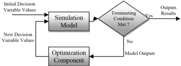
Optimization is a method normally applied to determine optimum values of system parameters (Long-Fei & Le-Yuan, 2013). That is, it is an approach that has to be applied to determine the optimum configurations of input parameters according to the output variables (Santucci & Capocchi, 2015). Employing the optimization in simulation models can help the result analysis of this model. It may happen as an optimization algorithm can be executed in order to avoid the trial-and-error use in the evaluation of the best scenarios of a simulation model (Chwif & Medina, 2010). There are various techniques of simulation optimization. Authors as Long-Fei & Le-Yuan (2013), Fu (2002) and ´Olafsson (2006) approach such techniques in their works. However, regardless the method used, the relation between simulation and optimization works the same way, Figure 1.

Figure 1– Relation between the simulation model and optimization. Source: adapted from Melouk (2013).

According to this Figure, the simulation model starts with variables of initial decisions. After executing the model, it is verified if the output results meet the stop criteria. In case the needs established are not satisfied, the output results return to the optimizator that uses the information to help select a new solution.

3 URURAU SOFTWARE

Ururau is a Free and Open-Source Software (FOSS) for DES, which uses Java Simulation Library (Rossetti, 2008). As commercial software is of high cost for small companies, Uru-rau is more accessible to assist them as it is a free software that can be accessed athttp: //ururau.ucam-campos.br. In addition to the basic models of discrete simulation, this

(4)

3.1 Calculation of emission

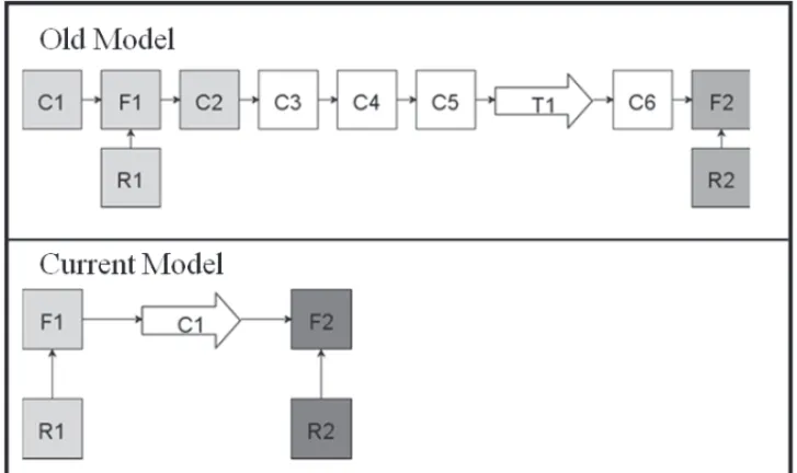
This software allows building models to calculate the gas emissions of vehicles in logistics systems in an easy way. The formula applied for calculation is based on the work of Zhou & Kuhl (2011). Figure 2 shows the same simulation model built in two different versions of the soft-ware and its improvement in calculating the emissions. In both versions, functions F1 and F2 and their resources R1 and R2 are only responsible for loading and unloading the vehicle. It can be observed, at the top of the Figure, the Old Model elaborated in version (0.5). Modules C1, C2, C3, C4, C5, T1 and C6, in this Figure, are responsible for the transportation and calculation of the emissions. At the bottom of the Figure, it can be seen the Current Model, formulated in actual version (1.0), composed of a single module in charge of the transportation of the load and the calculation of the gas emitted.

Figure 2– Old Simulation Model and Current Model.

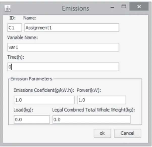
Developing a model of a logistics system in this model turned to be simpler. For instance, the emission of gases discharged from vehicles can be computed during the simulation. To use this module, it is necessary to insert data as the name of the variable that will accumulate the emis-sions and the parameters for the calculation itself (time, emission coefficient, engine power, load-ing of the vehicle and total gross weight). Figure 3 presents the module screen for the calculation of Emissions.

(5)

Figure 3– Emission module of URURAU software.

must have the unit in kg. It is highlighted that, for the calculation of the emissions, only the Emission Coefficient, Power and Time are needed. The Load and LCTWW work as a factor of compensation and take into consideration if the truck holds total or partial load.

3.2 Optimization function

As shown in Figure 4, an optimization module based on Genetic Algorithms (GA) was also developed. GAs are commonly used to solve Non-Deterministic Polynomial time (NP) problems. Pinho et al. (2012) applied an optimization method for DES models that uses GA; however, the authors compared the optimization method developed to a commercial optimization tool. With the optimization, it is possible to test different controlled variables in order to find the best result. Nevertheless, as GA is a metaheuristics method, it cannot guarantee optimum results but suboptimum ones.

(6)

be selected, otherwise, it will maximize. The parameters applied were the default of the JGAP library: elitist selector; crossover of aleatory point with rate of 35% concerning the population size; random mutation applied to 1 out of 12 genes in the entire population (Hall, 2013).

Figure 4– Optimization Module of the Ururau software.

4 DESCRIPTION OF THE SYSTEM

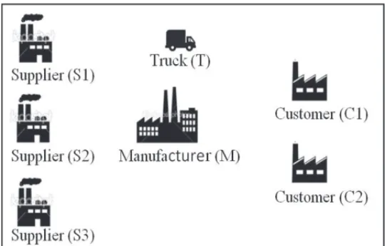
The system analyzed was based on the proposal of Rangel & Cordeiro (2015). The hypothetical system consisted of three suppliers, one manufacturer, two costumers and trucks to transport the load. Figure 5 illustrates the elements of this system.

Figure 5– Illustration of the system proposed to construct the model.

(7)

larger-sized, smaller-sized vehicles or both. It can also be observed that S1, S2, S3 represent the suppliers; M, the manufacturer; and C1, C2, the customers. These designations are the same for all configurations.

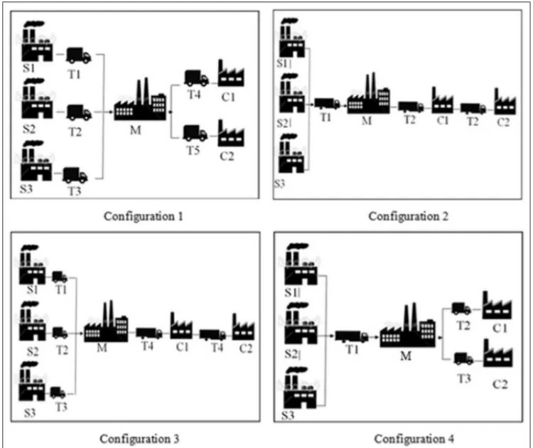
Figure 6– Illustration of configurations 1, 2, 3 and 4.

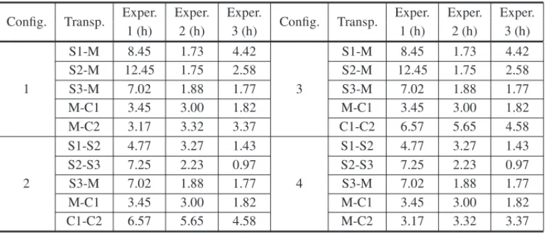
Table 1 presents the transportation times (obtained from Google Maps) of each element of the system for the four configurations. Experiments 1, 2 and 3 differ from each other in relation to the distance between the partners of the supply chain. However, there are many possible combi-nations, which can vary according to the local characteristics of each region. We chose to analyze three experiments for the evaluation.

In configuration 1, three small-sized trucks (T1, T2, T3) collect the material, one of each supplier (S1, S2, S3), transport and deliver it to the manufacturer (M). Two trucks (T4, T5) collect the finished products from the manufacturer and deliver them to their customers (C1 and C2).

(8)

Table 1– Time between the routes for configurations 1, 2, 3 and 4.

Config. Transp. Exper. Exper. Exper. Config. Transp. Exper. Exper. Exper. 1 (h) 2 (h) 3 (h) 1 (h) 2 (h) 3 (h)

1

S1-M 8.45 1.73 4.42

3

S1-M 8.45 1.73 4.42 S2-M 12.45 1.75 2.58 S2-M 12.45 1.75 2.58 S3-M 7.02 1.88 1.77 S3-M 7.02 1.88 1.77

M-C1 3.45 3.00 1.82 M-C1 3.45 3.00 1.82

M-C2 3.17 3.32 3.37 C1-C2 6.57 5.65 4.58

2

S1-S2 4.77 3.27 1.43

4

S1-S2 4.77 3.27 1.43 S2-S3 7.25 2.23 0.97 S2-S3 7.25 2.23 0.97 S3-M 7.02 1.88 1.77 S3-M 7.02 1.88 1.77

M-C1 3.45 3.00 1.82 M-C1 3.45 3.00 1.82

C1-C2 6.57 5.65 4.58 M-C2 3.17 3.32 3.37

Configuration 3 shows the collection of material from the supplier, which is done by three small-sized trucks (T1, T2, T3), one for each supplier. The material is unloaded in the manufacturer (M) and the distribution of the finished products to the costumers (C1, C2) is only done by one large-sized truck (T4), creating a route of various destinies.

Configuration 4 indicates the delivery of the material done by only one large-sized truck (T1), following a route among the suppliers. After collecting the finished products from the manufac-turer, the distribution takes place by means of two small-sized trucks (T2, T3) dispatching the products to each customer.

Thus, those configurations present the same elements. However, each one has different strategies, according to the logistics view. Then, it was possible to evaluate the impact of the variables chosen to the analysis in the routes presented.

5 SIMULATION MODEL

The methodology proposed by Banks et al. (2009) was used to construct the simulation model, where the following steps were applied: formulation and analysis of the problem; construction of the conceptual model; construction of the simulation model; verification and validation; experimentation and interpretation; statistical analysis of the results. The verification and val-idation of the simulation model followed the steps suggested by Sargent (2013). The IDEF-SIM language, presented by Montevechi et al. (2010), was used to the documentation of the concep-tual model of the system.

5.1 Elaboration of the model

(9)

search for the best configuration in relation to a specific objective. Nevertheless, a traditional analysis could also be possible. Each of the four configurations would have three scenarios, to-talling 12 experiments, that is, 12 simulation models. Using the optimization, there are only three simulation models, each with four configurations. Thus, the traditional analysis condition remains the same; however, the optimization algorithm returns the best configuration, avoiding the evaluation of the 12 experiments. Although the application of optimization of only 12 sce-narios is doubtful, the individual analysis of these scesce-narios would need more time and effort if the application of it were not employed. It is still important to highlight that, in case the number of configurations or scenarios increased, the quantity of analyses would increase significantly. Besides, another approach could be used, in which the parameter calculation was combined with another enumerator algorithm that emulated aleatory processes. However, it would demand a greater effort and more specific knowledge about programming to execute all the development steps of the model, mainly for the function of optimization. Thus, the use of the Ururau software makes the steps of development and analysis easier as the tool has the support of a simple and practical graphical interface.

The simulation model of each configuration was developed to meet a specific demand. In this case, the configurations do not run in closed systems. The vehicles pass through the system; dur-ing this time, they deliver the material, calculate the emissions and complete the process. There is a range of possible variations of logistics structures, each one with its own characteristics, from the simplest to the most complex. Though being a simple model, it shows the relation between environmental variables and traditional variables. This study is not meant to determine an over-all structure, but to demonstrate if there are trade-offs between variables analyzed, regardless of how the system behaves itself.

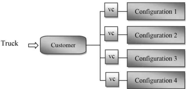
Figure 7 demonstrates schematically how the construction of the model was built when the con-figurations analyzed are included. The next elements were also observed: truck; decisor; variable of control (vc); and configurations. The principle of operation was as follows: the truck arrives at the decisor, which aims to direct its flow. The deviation to each configurations happens if the variable of control attends to a condition imposed, being this variable controlled by the optimiza-tion module. This way, each configuraoptimiza-tion is tested by the optimizaoptimiza-tion in relaoptimiza-tion to a specific purpose, which can be changed in function of any state variable registered by the simulation.

The fact that the inclusion of different configurations was carried out in a same model does not mean that the solution of the problem is the construction of a single model that aggregates different existent possibilities.

The following decision variables were applied as parameter for the optimization: Lead Time, Transport Time, Total Emission, being these ones obtained in the simulation, in which each variable was tested in the objective function. Figure 5 shows the optimization module used. In ‘Objective’, the expression f(x)=x1+x2+x3+x4was employed to minimize the emissions,

(10)

Figure 7– Layout of the proposed model with optimization integrated.

Despite the sum of the variables responsible by storing the emissions of each logistics structure in ‘Objective’, only one has an attributed value while the other ones are zero. This happens because of the ‘vc’ control that allows activating only one configuration at a time. Thus, they are evaluated individually. For the Lead Time and Transport Time, it is necessary to change the function of evaluation similarly. The computational model, from the illustration schematized in Figure 7, can be seen in Figure 8 in detail.

In Figure 8, the module E1, responsible for the creation of the entitites represented by vehicles, can be seen at the left margin. In the following sequence, there is the decisor symbolized by X, which leads the trucks according to a specific condition validated by the optimization algorithm. Modules LD, T1, T2, T3 and R1 are to calculate the Lead Time and Transport Time that are common to all configurations. However, there is the addition of L0 and L1 to the configurations 2 and 4 to limit the quantity of trucks of these structures. Modules J, J1 and J2, in configurations 2, 3 and 4, are to move the vehicles from one point to the other, in this case, used to better adjust the model to the layout of the screen.

In configuration 1, at the top of Figure 8, there is the decisor module X that just deviate the flow of vehicles by the predetermined percentage to each route. F1 and F2 represent respectively the loading and unloading of the material as well as F3, F4, F5, F6, F7, F9, F8 and F10. The modules R1 and R2 are the resources that the processes F1 and F2 use. R3, R4, R5, R6, R7, R8, R9, R10 are the resources applied in the loading and unloading step of the products. The calculation of the emissions and transportation of the products was done by modules C1, C2, C3, C4 and C5.

(11)

Figure 8, at the central part, presents the configuration 3, in which the decisor module X only deviates the vehicle flow according to the percentage specified for each route. Modules F1, F3, F5 and F7 represent the loading process of the products, and R1, R3, R5 and R7 are their re-spective resources. The unloading process is executed by modules F2, F4, F6, F8 and F9 and their resources R2, R4, R6, R8 and R9. The calculation of the emissions and transportation of the products was done by the modules C1, C2, C3, C4 and C5.

To conclude, at the bottom part of Figure 8, there is the configuration 4, where modules F1, F2, F3, F5 and F7 are responsable for the loading of the material and R1, R2, R3, R5 and R7, for resources. The unloading function of the material is executed by F4, F6 and F8, where R4, R6 and R8 are the resources used for these processes. The decisor X only deviates the flow of the vehicles in accordance to the percentage stipulated for each route. The calculation of the emissions and transportation of the material was done by the modules C1, C2, C3, C4 and C5.

5.2 Inclusion of multivariable in the objective function

The optimization system employed can only run with one type of variety in the objective func-tion, which is the traditional way. In this step, an adaptation of the objective function was pro-posed with the aim to include more than a type of variable. To this end, a different structure was performed in this function. The variables Lead Time, Transport Time and Total Emission were included as well as weight for each one. For this purpose, a correction was done, that is, the value of the variable Total Emission was divided by 1000 to reduce its order of magnitude. That is because of its high value, which made it much sensitive to small stochastic oscillations. It is important to highlight that we are not working with multiobjective optimization methods but rather on an adaptation in the objective function. Thus, the following expression was elaborated to include the three variables and their weights in the objective function:

X∗_LeadTime_(i)+Y∗_{TransportTime}_(i)+Z∗_{(TotalEmission}_(i)/1000)

whereX,Y,Zare the weights established for each criterion; andirepresents the configurations, beingi >0.

It is worth remembering that the total sum, when executed in the objective function of opti-mization, computes only one configuration per time, attributing zero to the variables of different configurations. Then, the variables of a configuration do not influence on the others.

(12)

(13)

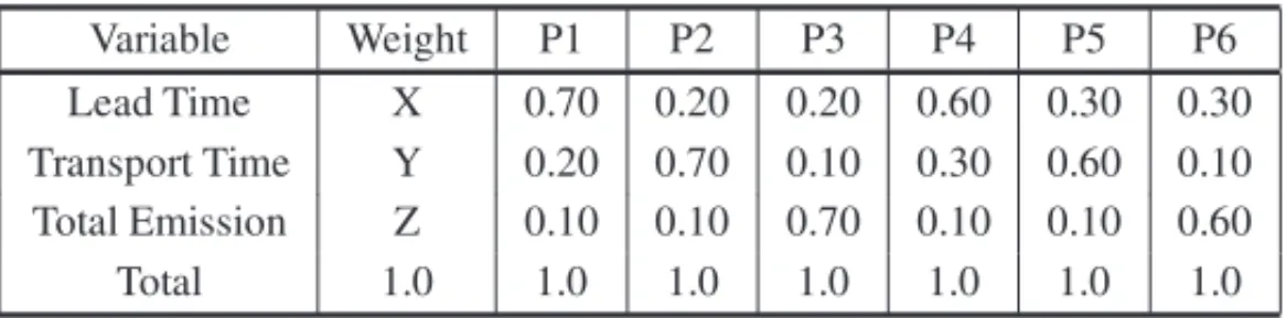
Table 2– Related weights for optimization.

Variable Weight P1 P2 P3 P4 P5 P6 Lead Time X 0.70 0.20 0.20 0.60 0.30 0.30 Transport Time Y 0.20 0.70 0.10 0.30 0.60 0.10 Total Emission Z 0.10 0.10 0.70 0.10 0.10 0.60 Total 1.0 1.0 1.0 1.0 1.0 1.0 1.0

Different from Table 2, Table 3 shows the values generated randomly in a spreadsheet. They were also tested in the objective function of the optimization. Moreover, those values can be used to study the behavior of the model for each weight group.

Table 3– Random weights tested in the optimization function.

Variable Weight P7 P8 P9 P10 P11 P12 P13 P14 P15 Lead Time X 0.40 0.26 0.79 0.65 0.40 0.62 0.19 0.51 0.05 Transport Time Y 0.27 0.38 0.12 0.22 0.25 0.11 0.37 0.24 0.27 Total Emission Z 0.33 0.36 0.09 0.13 0.35 0.27 0.44 0.25 0.68 Total 1.0 1.0 1.0 1.0 1.0 1.0 1.0 1.0 1.0 1.0

5.3 Execution parameters of the simulation model

The simulation model execution was performed in a Dell Inspiron – IntelCoreTMprocessor i3-4130 CPU3,4GHz, Windows 8.1 Operating System 64 bits.

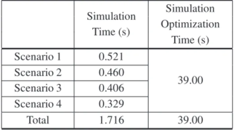
The number of replications was determined when the results converged, stabilizing with 30 repli-cations. The simulation run was of 250 hours and the simulation time can be seen in Table 4. The simulation time with optimization of the models was of 39s. The total time of simulation of the models (with no optimization) was of 1.716s, that is, 22.7 times lower than the optimization time. In spite of it, this time of computational convergence is considered efficient for the opti-mization algorithm. The other rounds of the experimentation step had times quite close to those here presented.

6 SIMULATED EXPERIMENTS

(14)

Table 4– Time of simulation with and without optimization.

Simulation Simulation Time (s) Optimization

Time (s) Scenario 1 0.521

39.00 Scenario 2 0.460

Scenario 3 0.406 Scenario 4 0.329

Total 1.716 39.00

6.1 Simulation optimization model

Table 5 displays three experiments and four configurations, where the means and the standard deviation (SD) of the Lead Time, Transport Time and Emission variables are presented. The optimum values are highlighted by the circles among the configurations of each experiment. After executing the simulation model via optimization with the four configurations used, only the 1 and the 3 were indicated by the optimization. That is, configuration 1 showed the lowest Emission and Transport Time, and configuration 3, the least Lead Time. Despite the algorithm used being a metaheuristic, the results found were optimum as can be checked in Table 5. That probably happened because of the small space of search.

Table 5– Results of the best configurations after the simulation with optimization.

Experiment 1 Config. 1 S. D Config. 2 S. D Config. 3 S. D Config. 4 S. D Lead Time 82.39 2.64 102.29 3.77 67.55 1.80 90.84 3.12 Transport Time 12.61 0.71 29.03 1.40 19.15 1.45 22.68 0.98 Emission 33279.27 3320.65 48533.00 2414.92 45093.52 3334.84 59311.46 2991.23 Experiment 2 Config. 1 S. D Config. 2 S. D Config. 3 S. D Config. 4 S. D

Lead Time 78.15 5.39 88.69 0.54 64.31 1.11 78.16 0.86 Transport Time 5.02 0.10 16.23 0.30 10.58 0.27 10.67 0.18 Emission 14080.18 348.10 24117.10 426.55 17433.39 446.46 23176.13 334.60

Experiment 3 Config. 1 S. D Config. 2 S. D Config. 3 S. D Config. 4 S.D Lead Time 77.71 5.42 84.31 0.513 63.08 1.124 75.64 1.01 Transport Time 5.41 0.30 10.6 0.412 9.32 0.74 6.75 0.29 Emission 15129.92 1002.67 16022.39 505.64 17720.12 1189.96 16840.10 562.92

(15)

Figure 9 shows the comparison between the Lead Time and Total Emission of the best logistics configurations found for this problem. The chart generated in the Figure has three experiments and two configurations, where a line in dark grey, which represents the Lead Time, and bars in the vertical in light grey that show the total emission are identified. For all experiments, the values of these variables oppose among the configurations, that is, are inversely proportional, but present different proportions for each experiment.

Figure 9– Comparison between the Emission and Lead Time variables.

When observing Figure 9, it can be seen that configuration 1 presented lower emission but higher Lead Time for all experiments. However, configuration 3 showed shorter Lead Time and higher emission. Observing the chart in this Figure, we are able to check that experiment 1, compared to the 2 and the 3, exposes a higher variation in the emissions; but in the Lead Time, these divergences are less; that is because one of the factors that affects this variable, besides the time of transport, is the step of loading and unloading. These steps work as a bottleneck retaining the vehicle flow. In this manner, the different positions of the suppliers, manufacturers and customers do not cause much impact in the Lead Time like the steps of the load processing (loading and unloading) for this problem.

The chart in Figure 10, in which the advance rank of the configurations are represented, shows the trade-offs between configurations 1 and 3 of the experiments carried out. The bars, in dark grey, represent the Lead Time, and the ones in light grey, the Total Emissions. In general, it was seen that each configuration opposes, displaying its advantages and disadvantages.

(16)

In experiment 2, there is an increase of 24% in the emissions and a decrease of 18% in the Lead Time when configuration 3 in relation to 1 is analyzed. Although, when verifying 1 concerning 3 (1/3), there is a decrease of 19% in the emissions and an increase of 22% in the Lead Time.

In experiment 3, when analyzing configuration 3 related to 1 (3/1), there was an increase of 16% in the emissions and a decrease of 19% in the Lead Time; despite that, when configuration 1 is checked in relation to 3 (1/3), there is a reduction of 14% in the emissions and an increase of 23% in the Lead Time.

Again, in Figure 10, each configuration is inversely proportional to the other because of the conflictive objectives. That happens because each strategy has different characteristics as routes and kinds of vehicles. For instance, while some prioritize a faster delivery, others emphasize the highest number of transported volume. Then, it is noticed that, apart from the experiments carried out, the relation of trade-off was kept. It should be stressed that probably in a supply chain with more links and vehicles traveling in different ways, it can present different results from the ones already found, but the trade-off relation would be preserved once the strategies adopted have conflicting objectives.

The number of configurations analyzed was reduced when using simulation optimization. Between the four ones, only two were selected, as they were more efficient to the intended objectives; that did the analysis and the detailed interpretation of data easier, once it reduced the number of alternatives evaluated. Thus, time and resources were minimized for the analysis of this problem.

Figure 10– Advance rate of a logistics structure in relation to other.

6.2 Attributing weights to the variables of state

(17)

Three groups of weights and their criteria, in which each group prioritizes a different variable for the four configurations, are observed in Table 6. This Table is the result of multiplying the weights by the values of the variables of experiment 1 of Table 5. The process of choosing the configuration was simple. The one that presented the least total value was chosen as the best one. This way, the result of the Table was contrasted with the one returned by the simulation optimization.

When placing priority on the Lead Time, in Table 6, configuration 3 was chosen because it pre-sented the least total value. Prioritizing Transport Time and Total Emission, configuration 1 was elected. The selection of these configurations by the optimization was the same when analyzing only one criterion at a time.

Table 7 is the prolongation of Table 6 and both have the same function of testing the behavior of the variables in relation to the weight established; however, Table 7 shows a synthesized layout for the execution of more experiments. Here, weights from 4 to 8 were tested, which can be seen in Tables 2 and 3. All iterations can be found in Appendix B.

Table 6– Configuration results considering the weights for each criterion.

Prioritizing Lead Time

Criteria&Weights-1 Config. 1 Config. 2 Config. 3 Config. 4 Lead Time (0.7) 57.22 71.60 47.28 63.59 Transport Time (0.2) 2.52 5.81 3.83 4.54 Total Emission (0.1) 3.33 4.85 4.51 5.93 Total 63.07 82.26 55.62 74.05

Prioritizing Transport Time

Prioritizing Total Emission

(18)

Table 7– Synthesized results of the configurations considering the weights for each scenario.

Weights Conf. Lead Transport Total Total Weights Conf. Lead Transport Total Total

Time Time Emission Time Time Emission

4

1 49.04 3.78 3.33 56.15

7

1 32.43 3.44 10.99 46.86

2 60.70 8.71 4.85 74.26 2 40.13 7.93 16.03 64.08 3 40.53 5.74 4.51 50.78 3 26.80 5.23 14.89 46.92 4 54.50 6.80 5.93 67.24 4 36.03 6.19 19.59 61.81

5

1 24.52 7.56 3.33 35.41

8

1 21.35 4.82 11.85 38.02

2 30.35 17.42 4.85 52.62 2 26.43 11.11 17.28 54.82 3 20.26 11.49 4.51 36.26 3 17.65 7.33 16.05 41.03 4 27.25 13.61 5.93 46.79 4 23.73 8.68 21.11 53.52

6

1 24.52 1.26 19.97 45.75

– 2 30.35 2.90 29.12 62.37

3 20.26 1.91 27.06 49.24 4 27.25 2.27 35.59 65.11

The following Figure 11 represents the chart of the absolute and relative total values of the configurations for each weight group relating to Table 7. The dark grey line symbolizes the relative variations of each weight group while the light grey bars typifies the absolute ones. Note that the absolute values display differences between their groups. However, the changes are minimum in the relative values when comparing the respective configurations of one group with the other.

For each group of weights, configurations 1 and 3 stand out regarding a lower total value. In absolute terms, it can be seen a variation that does not follow a proportion between each group. However, when analyzing the relative values, they follow an oscillation almost proportional with a difference around 2% for the same configurations in each group. That means that the differ-ent total variations of each group of weights did not force or persuade the choice of a specific configuration by the optimization.

6.3 Comparison between optimization and Analytic Hierarchy Process (AHP)

Using the optimization method, which considered more than one criterion in the objective func-tion establishing weights for those criteria, it was able to achieve a particular result. Thus, it was opted to use the AHP multicriteria method proposed by Saaty (2003) that also aims to choose an alternative that better adapts to the criteria and established weight. The objective was to identify if the results converged with those of the optimization. Figure 12 shows the hierarchical struc-ture proposed. The intention is to choose the best configuration, in which three criteria and four alternatives are analyzed.

(19)

Figure 11– Absolute and relative total values of each scenario for the weight groups of Table 7.

Figure 12– Hierarchy of the proposed problem.

alternatives, the configurations. The comparison of the alternatives was done using the values of experiment 1 of Table 5. In the comparison of the criteria, the weights of Tables 2 and 3, which are the same of the simulation optimization, were applied.

(20)

Table 8– Comparative between the answer of the simulation model with optimization and the AHP method.

Weights Simulation Optimization AHP Weight 4 Configuration 3 Configuration 3 Weight 5 Configuration 1 Configuration 1 Weight 6 Configuration 1 Configuration 1 Weight 7 Configuration 1 Configuration 3 Weight 8 Configuration 1 Configuration 1 Weight 9 Configuration 3 Configuration 3 Weight 10 Configuration 3 Configuration 3 Weight 11 Configuration 1 Configuration 3 Weight 12 Configuration 3 Configuration 3 Weight 13 Configuration 1 Configuration 1 Weight 14 Configuration 3 Configuration 3 Weight 15 Configuration 1 Configuration 1

The results between the methods, in Table 8, are the same for Weights 4, 5, 6, 8, 10, 12, 13, 14 and 15. However, there is a difference between the methods employed when Weights 7 and 11 were applied. For both Weights 7 and 11, configuration 1 was chosen when using simulation opti-mization, whereas configuration 3 worked better in the AHP. This divergence happened possibly because of the total values that were really close between configurations 1 and 3. For Weight 7, the values were of 46.86 for scenario 1 and 46.92 for scenario 2, whereas for Weight 11, were of 47.49 for scenario 1 and 47.59 for scenario 3. The percentage difference between configu-rations 1 and 3 for Weights 7 and 11 are, respectively, 0.13% and 0.21%. Therefore, the AHP method was not so sensitive to capture those subtle differences.

7 CONCLUSIONS

We evaluated in detail the behavior of the economic and environmental variables in logistics sys-tems searching to find more answers concerning works published in the literature. This way, the relation of direct proportionality among the variable emissions, transport time and lead time was found; however, it was also identified that the process time of loading may affect that relation of proportionality. Those variables presented inverted relation when compared to different configu-rations because each configuration had different vehicles, routes and times of load processing.

(21)

We adapted the objective function of the optimization algorithm, considering weights for the Lead Time, Transport Time and Total Emission criteria. This way, it was possible to compare the results of the simulation optimization with the AHP method. Both methods converged to the same results except when alternatives evaluated presented different percentages of 0.13% and 0.21%. Thus, the mathematical method of optimization was numerically more exact.

The use of AHP method was a way to validate the adaptation performed in the objective function and proved to be adherent to the problem. If the AHP method was applied to the results of the simulation, very similar alternatives to those of the simulation optimization would be achieved. However, there is the necessity to run more tests as we cannot generalize it to other applications with optimization once it was used in a specific problem.

Despite having been experimented in an only model with different internal configurations for the load transportation, the study indicates that, when evaluating economic and environmental (gas emissions) aspects, the research needs to be carried out carefully. What can be seen is that, in this type of analysis, it is recommended to make models that involve the different options that we can have to do the transportation of the load. That is because, according to the logistics system adopted, we can achieve conflicting results between the development variables of the system and the environmental ones.

It is worthwhile highlighting that the information of the relation between gas emission and de-livery time may be a useful information. That kind of information may help the manufacturer and the final customer make environmentally correct decisions. The manufacturers, for instance, can choose sustainable logistics strategies. Moreover, the customers should be advised that the choice for a faster delivery of the product purchased may be causing a higher greenhouse gas emission during the load transport. Consequently, a conscious consumer may opt for waiting for the product during a longer period and, subsequently, take a more sustainable decision benefit-ting the planet.

REFERENCES

[1] BALLOURH. 2004. Business Logistics/Supply Chain Management. 5th Edition, New Jersey: Pren-tice Hall.

[2] BANKSJ, CARSON II JS, NELSONBL & NICOL D. 2009. Discrete-event System Simulation, 5th ed. Prentice-Hall: Englewood Cliffs, NJ.

[3] BYRNEPJ, HEAVEYC, RYANP & LISTONP. 2010. Sustainable supply chain design: capturing dynamic input factors.Journal of Simulation,4(4): 213–221.

[4] CHWIFL & MEDINAAC. 2010. Modelagem e Simulação de Eventos Discretos: Teoria e Aplicações. São Paulo: Ed. dos Autores, 309 p.

(22)

[6] DAGKAKIS G & HEAVEY C. 2015. A review of open source discrete event simulation soft-ware for operations research. Journal of Simulation advance online publication, 19 June 2015; doi:10.1057/jos.2015.9.

[7] FUMC. 2002. Optimization for Simulation: Theoryvs.Practice.Journal on Computing,14(3): 192– 215.

[8] FUMC, ANDRADOTTIR´ S, CARSONJS, GLOVERF, HARRELLR, HOYC, KELLY JP & ROBIN

-SONSM. 2000. Integrating optimization and simulation: research and practice. InProceedings of the Winter Simulation Conference, edited by JOINESJA, BARTONR, KANGK & FISHWICKPA, 610-616. Piscataway, New Jersey: Institute of Electrical and Electronics Engineers, Inc.

[9] HALLM. 2013. JGAP Default Initialisation Configuration. http://mathewjhall.wordpress.com/2013/ 02/18/jgap-default-initialisation. Accessed 14 July 2016.

[10] IEA STATISTICS. 2014. CO2 emissions from fuel combustion-highlights.http://www.iea.

org/publications/freepublications/publication/CO2Emissions From

Fuel-CombustionHighlights2014.pdf. Accessed 27 February 2015.

[11] JAEGLER A & BURLATP. 2012. Carbon friendly supply chains: a simulation study of different scenarios.Production Planning & Control,23(1): 269–278.

[12] KELTOND, SADOWSKIRP & STURROCKDT. 2007. Simulation with Arena. 4 ed., New York, NY, USA: Mc Graw Hill.

[13] KINGDH & HARRISONHS. 2013. Open-Source Simulation Software JAAMSIM. InProceedings of the Winter Simulation Conference, edited by PASUPATHYR, S-HKIM, TOLKA, HILLR & KUHL

ME, 2163-2171. Piscataway, New Jersey: Institute of Electrical and Electronics Engineers, Inc.

[14] LONGOF. 2012. Sustainable supply chain design: an application example in a local business retail. Simulation,88(12): 1484–1498.

[15] LONG-FEI, WANG& LE-YUANSHI. 2013. Simulation optimization: a review on theory and appli-cations.Acta Automatica Sinica,39(11): 1957–1968.

[16] MELOUKSH, FREEMANNK, MILLER D & DUNNINGM. 2013. Simulation optimization-based decision support tool for steel manufacturing. International Journal of Production Economics,

141(1): 269–276.

[17] MONTEVECHIJAB, LEALA, PINHOA, COSTARF, OLIVEIRAML & SILVAAL. 2010. Concep-tual Modeling in Simulation Projects by mean adapted IDEF: an Application in a Brazilian company. InProceedings of the Winter Simulation Conference, edited by JOHANSSONB, JAINS, MONTOYA -TORRESJ, HUGANJ & Y ¨UCESANE, 1624-1635. Piscataway, New Jersey: Institute of Electrical and Electronics Engineers, Inc.

[18] O´LAFSSONS. 2006. Metaheuristics. In: HENDERSONSG & NELSONBL (Eds.),Handbooks in operations research and management science: Simulation (pp. 633–654). Amsterdam: Elsevier Sci-ence.

[19] PEIXOTO TA ET AL. 2016. Ururau: a free and open-source discrete event simulation software. Journal of Simulation, p. 1–19. (doi:10.1057/s41273-016-0038-5)

(23)

[21] RAMANATHANU, BENTLEY Y & PANGG. 2014. The role of collaboration in the UK green sup-ply chains: an exploratory study of the perspectives of suppliers, logistics and retailers.Journal of Cleaner Production,70(1): 231–241.

[22] RANGELJJA & CORDEIROACA. 2015. Free and Open-Source Software for Sustainable Analysis in Logistics Systems Design.Journal of Simulation(Print),9(1): 27–42.

[23] RIZET C & KE¨ITAB. 2005. Chaˆınes logistiques et consommation d’´energie: cas du yaourt et du jean. Rapport de recherche. 92 p.

[24] ROSSETIMD. 2008. Java Simulation Library (JSL): An Open-Source Object-Oriented Library for Discrete-Event Simulation in Java.International Journal of Simulation and Process Modelling,4(1): 69–87.

[25] SAATY TL. 2003. Decision-making with the AHP: Why is the principal eigenvector necessary? European Journal of Operational Research,145(1): 85–91.

[26] SANTUCCIJF & CAPOCCHIL. 2015. Optimization via simulation of catchment basin management using a discrete-event approach.Simulation,91(1): 43–58.

[27] SARGENTRG. 2013. Verifications and validation of simulations models.Journal of Simulation,7(1): 12–24.

[28] UNFCCC (UNITEDNATIONSFRAMEWORKCONVENTION ONCLIMATECHANGE). 1997. Kyoto Protocol to the United Nations Framework Convention on Climate Change.http://unfccc. int/kyoto\_protocol/items/2830.php. Accessed 22 July 2015.

(24)

Appendix A– Description of the conceptual model.

Module Description Module Parameters

E1 Responsible for the T. Arrivals: Const. (1 h) creation of entities T. First Arrival: 0.0 h

Max. Arrivals: 20

X Decide Type: N-way-by-condition

Expression (1) if true: c= = 1 Expression (2) if true: c= = 2 Expression (3) if true: c= = 3

Expression (4) if false

Configuration 1 Configuration 2

LD Adds an Type: Attribute L0 Adds a Type: variable attribute to Attribute Name: leadtime variable to Variable Name: C2S2

the model Value: TNOW the model Value: C2S2+1 X Decides Type: N-way-by-chance L1 Hold Expression if true:

1-Rate if true %: 30 C2S2¡=7

2-Rate if true %: 30 3-Rate if: false

F1 Executes Type: Expression LD Adds an Type: Attribute a process Value: (20,000/4,000) attribute to Attribute Name: leadtimeS2

the model Value: TNOW F2 Executes Type: Expression F1 Executes Type: Expression

a process Value: (20,000/6,000) a process Value: (20000/4000) F3 Executes Type: Expression F2 Executes Type: Expression

a process Value: (10,000/6,000) a process Value: (50000/4000)

X Decide Type: 2-way-by-chance J Jump –

1-Rate if true %: 50 2-Rate if: false

F7 Executes Type: Expression F6 Executes Type: Expression a process Value: (46,000/4,000) a process Value: (25000/6000) F8 Executes Type: Expression F7 Executes Type: Expression

a process Value: (46,000/4,000) a process Value: (25000/6000) F9 Executes Type: Expression C1 Calculates Variable name: var1S2

a process Value: (23,000/4,000) the emissions Time(h):NORM(4.77,1.5) Emissions coefficient: 1.5

Power: 265 Load(kg): 20,000 Legal Combined Total Whole

(25)

Appendix A– Description of the conceptual model (continuation).

Max. Arrivals: 20

F10 Executes Type: Expression C2 Calculates Variable name: var1S2 a process Value: (23,000/4,000) the emissions Time(h):NORM(7.25,2.0)

Emissions coefficient: 1.5 Power: 265 Load(kg): 45,000 Legal Combined Total Whole

Weight(kg): 56,000 C1 Calculates Variable name: var1 C3 Calculates Variable name: var1S2

the emissions Time(h):NORM(8.85,2.0) the emissions Time(h):NORM(7.02,2.0) Emissions coefficient: 1.5 Emissions coefficient: 1.5

Power: 136 Power: 265

Load(kg): 20,000 Load(kg): 55,000

Legal Combined Total Whole Legal Combined Total Whole Weight(kg): 30,000 Weight(kg): 56000 C2 Calculates Variable name: var1 C4 Calculates Variable name: var1S2

Load(kg): 23,000 Load(kg): 50,000

Legal Combined Total Whole Legal Combined Total Whole Weight(kg): 30,000 Weight(kg): 56000 C3 Calculates Variable name: var1 C5 Calculates Variable name: var1S2

Load(kg): 10,000 Load(kg): 25,000

Legal Combined Total Whole Legal Combined Total Whole Weight(kg): 30,000 Weight(kg): 56000 C4 Calculates Variable name: var1 T1 Adds a Type: variable

the emissions Time(h):NORM(3.45,1.0) variable to Variable Name: sumS2 Emissions coefficient: 1.5 the model Value:EMISSION LEAD

Power: 136 TIME+sumS2

Load(kg): 10,000 Legal Combined Total Whole

(26)

Appendix A– Description of the conceptual model (continuation).

Max. Arrivals: 20

C5 Calculates Variable name: var1 T2 Adds a Type: variable the emissions Time(h):NORM(3.17,1.0) variable to Variable Name: countS2

Emissions coefficient: 1.5 the model alue: countS2+1 Power: 136

Load(kg): 23,000 Legal Combined Total Whole

Weight(kg): 30,000

T1 Adds a Type: variable T3 Adds a Type: variable variable to Variable Name: sum variable to Variable name: transportS2 the model Value:EMISSION LEAD the model Value: sumS2/(count)

TIME+soma

T2 Adds a Type: variable R1 Lead Type: Time Interval variable to Variable Name: count Time Attribute: leadtimeS2 the model Value: count+1

— — — R1 up to R7 Resource Capacity 1

T3 Adds a Type: variable variable to Variable Name: transport the model Value: sum/(count) R1 Lead Type: Time interval

Time Attribute: leadtime —

(27)

Appendix B– Results of the scenarios considering the weights for each criterion.

Weights Conf. Lead Transport Total Total Weights Conf. Lead Transport Total Total

Time Time Emission Time Time Emission

4

1 49.04 3.78 3.33 56.15

10

1 53.35 2.81 4.13 60.29 2 60.70 8.71 4.85 74.26 2 66.03 6.48 6.02 78.53 3 40.53 5.74 4.51 50.78 3 44.09 4.28 5.59 53.96 4 54.50 6.80 5.93 67.24 4 59.29 5.06 7.35 71.71

5

1 24.52 7.56 3.33 35.41

11

1 32.70 3.15 11.65 47.49 2 30.35 17.42 4.85 52.62 2 40.46 7.26 16.99 64.71 3 20.26 11.49 4.51 36.26 3 27.02 4.79 15.78 47.59 4 27.25 13.61 5.93 46.79 4 36.33 5.67 20.76 62.76

6

1 24.52 1.26 19.97 45.75

12

1 50.32 1.44 8.99 60.75 2 30.35 2.90 29.12 62.37 2 62.27 3.32 13.11 78.70 3 20.26 1.91 27.06 49.24 3 41.58 2.19 12.18 55.95 4 27.25 2.27 35.59 65.11 4 55.92 2.59 16.03 74.53

7

1 32.43 3.44 10.99 46.86

13

1 15.82 4.72 14.38 34.91 2 40.13 7.93 16.03 64.08 2 19.57 10.87 20.97 51.41 3 26.80 5.23 14.89 46.92 3 13.07 7.17 19.48 39.72 4 36.03 6.19 19.59 61.81 4 17.58 8.49 25.62 51.69

8

1 21.35 4.82 11.85 38.02

14

1 41.30 3.08 8.33 52.71 2 26.43 11.11 17.28 54.82 2 51.11 7.10 12.15 70.35 3 17.65 7.33 16.05 41.03 3 34.13 4.68 11.29 50.10 4 23.73 8.68 21.11 53.52 4 45.90 5.54 14.84 66.28

9

1 64.22 1.61 2.90 68.72

15