http://www.journalofmoneyinvestmentandbanking.com
The New Keynesian Model:
An Empirical Application to the Euro Area Economy
Ricardo BarradasDinâmia’CET-IUL and ISCTE – University Institute of Lisbon
Higher School of Communication and Media Studies (Polytechnic Institute of Lisbon) Higher Institute of Accounting and Administration of Lisbon (Polytechnic Institute of Lisbon)
E-mail: rbarradas@escs.ipl.pt / rpbarradas@iscal.ipl.pt Abstract
This paper empirically applies the New Keynesian Model to the euro area’s economy during the period from the first quarter of 1999 to the last quarter of 2008, which is consistent with the scant empirical evidence on this Dynamic Stochastic General Equilibrium model. The New Keynesian Model is estimated using the Generalized Method of Moments, since the model denote hybrid features including backward and forward looking behaviours by economic agents and elements with rational expectations. Although this method of estimation may present some limitations, the New Keynesian Model seems to describe reasonably well the evolution of economic activity, the inflation rate and monetary policy in the euro area. Against this backdrop, the New Keynesian Model may provide an important tool for aiding the governments of euro area countries and the European Central Bank in the adoption and implementation of its policies over time.
Keywords: New Keynesian Model, IS Curve, Phillips Curve, Taylor Rule, Generalized Method of Moments, Euro Area
JEL CLASSIFICATION: C22 and E52
1. Introduction
In recent years, the New Keynesian Model (NKM) has gained credibility and a huge empirical
preponderance as a theoretical and practical framework to analyse the major macroeconomic dynamics and/or relationship between monetary policy, economic performance and the evolution of general prices. The NKM rests on solid microeconomic foundations, reflecting the optimising behaviour of economic agents.
In general terms, the NKM represents a small macroeconomic model, commonly referred to as a Dynamic Stochastic General Equilibrium model, which is formally structured into three equations that attempt to describe the evolution of aggregate demand (IS Curve), the inflation rate (Phillips Curve) and short-term nominal interest rate (Taylor Rule), as shown by Yun (1996), Goodfriend and King (1997), Rotemberg and Woodford (1995, 1997), McCallum and Nelson (1999) and Clarida et al. (1999), among others.
In this regard, the IS Curve describes the dynamics of output, representing aggregate demand in the economy, which derives from the decisions of households in present and future utility maximisation. The Phillips Curve illustrates the behaviour of the inflation rate over time and represents the supply side of the economy, deriving from firms’ behaviour in relation to profit maximisation. Finally, the Taylor Rule sets the evolution of short-term nominal interest rates over time, arising from
the decisions of monetary policy authorities on the maximisation of full employment and/or price stability.
However, the empirical application of the NKM to the euro area is relatively scarce, due to the short history of this monetary union and, therefore, the inexistence of historical aggregated data for the euro area. Nevertheless, Peersman and Smets (1999) and Gerlach and Smets (1999) estimate backward looking versions of the IS Curve and Phillips Curve, while Galí et al. (2001 and 2005) provide more recent empirical evidence but focus exclusively on the Phillips Curve. Further, Gerdesmeier and Roffia (2003) estimate a set of reaction functions for monetary policy created by the European Central Bank (ECB). However, these authors use a set of data (aggregated by themselves) for periods prior to the euro area creation. Therefore, their findings refer to a kind of “virtual” euro area that does not formally exist and whose major economies have not even met the conditions for this in accordance with the Maastricht Criteria.
Against this backdrop, this paper applies the NKM to the euro area’s economy, contributing to the literature through the utilization of aggregated data for the first 10 years of this economy as a whole. Moreover, we adopt the hybrid version of the NKM because the canonical version (that incorporates only the forward looking version) has demonstrated a reduced ability to replicate the behaviour of most macroeconomic variables over time, as stressed by Ball (1991) and Fuhrer (1997). Thus, the IS Curve, the Phillips Curve and the Taylor Rule are estimated individually using the Generalized Method of Moments (GMM), not only due to the incorporation of hybrid features, but also due to the presence of rational expectations. Moreover, this method of estimation also allows us to circumvent the problem of endogeneity between variables.
Overall, our study suggests that the hybrid version of the NKM replicates considerably well aggregate demand, the inflation rate and monetary policy conducted by the ECB in the first 10 years of the euro area. However, we were also able to identify that output and the inflation rate in the euro area denote a certain level of persistence. Moreover, monetary policy has been steered with an expressive degree of inertia.
The remainder of this paper is organised as follows. Section 2 defines the theoretical background of the NKM as well as the microeconomic foundations of the IS Curve, Phillips Curve and Taylor Rule. In Section 3, we describe the econometric method and the data. In Section 4, the main results are presented and discussed. Finally, Section 5 concludes.
2. The New Keynesian Model: Theoretical Background
The NKM arrived between the end of the sixties and the beginning of the seventies, seeking to answer the gaps in classic and/or Keynesian models that, until then, dominated the picture of economic thought and the orientation procedures of governments and international monetary authorities.
Consider that “our first and most important point is that existing Keynesian macroeconometric models
cannot provide reliable guidance in the formulation of monetary, fiscal, or other types of policy. This conclusion is based in part of the spectacular recent failures of these models and in part on their lack
of a sound theoretical or econometric basis” (Lucas and Sargent, 1979, p. 16).
Indeed, the assumptions of perfectly competitive markets, fully flexible prices and adaptive expectations by economic agents seemed slightly at odds with the social-economic reality, necessitating the emergence of a new stream of thought that was more consistent with the optimisation behaviour of economic agents and more able to characterise the relationship between monetary policy, the evolution of economic activity and inflation dynamics over time.
In fact, the NKM emerged essentially to provide microeconomic foundations for the postulates of classic and/or Keynesian economic models. Notice that the neo-Keynesian paradigm sustains, namely that households and firms have rational expectations (formed on basis of all available information and, therefore, unbiased) instead of adaptive expectations (formed simply and mechanically based exclusively on lagged information). This paradigm further assumes that business
cycles (or the fluctuations in real output over time) are the result of economic system failures, in a context where imperfections and/or market frictions prevent the economy from reaching, by itself, efficient levels of production and employment.
Against this background, market frictions may represent important mechanisms of propagation, amplifying shocks or disturbances that cause business cycles. Thus, neo-Keynesian economists argue that macroeconomic stabilisation by governments (through budgetary or fiscal policies) and/or by central banks (through monetary policies) lead to more efficient results than the results of laissez-faire policies.
The NKM admits that households from a specified economy, with an infinite life, offer their workforce and buy goods for their own consumption or save the income earned and/or the money they have. By contrast, firms in this same economy hire workers, produce and offer differentiated products in an imperfect market characterised by monopolistic competition (differentiation could be due to the appearance, quality, location or other attributes of the products). Moreover, all this occurs in a context where each firm fixes the price of the goods it produces (firms are “price-makers”) but not all review the price in each period of time, which can present, thus, some rigidity (“sticky prices”). This form of price adjustment was presented by Calvo (1983), whereby some firms update their prices in each period, while the remaining keep them unchanged due to the costs incurred in the process of the adjustment of prices and wages (“staggered prices” and “menu costs”).
Owing to the nominal rigidity of prices and wages, changes in short-term interest rates by the monetary authority no longer influence the inflation rate in the short-term by exactly the same proportion, but only at the level of real interest rates. This ends up affecting immediate consumption, investment and employment (or, ultimately, economic activity) because firms prefer to adjust the amount of offered products to the new level of aggregate demand (the principle of the non-neutrality of monetary policy). Meanwhile, neo-Keynesian economists preserve the utilisation of expansionary monetary policies for macroeconomic stabilisation purposes, warning that they should not be used (only) to create short-term benefits, which could lead to an increase in inflation expectations with adverse consequences in the future. In that sense, both households and firms display optimal behaviour. Households seek to maximise their present and future utility and firms attempt to maximise their profits given the technology available and the competition they face from other firms in the market.
Finally, the NKM also assumes the existence of a central bank that is responsible for monetary policy and, therefore, the fixation of nominal interest rates in the economy. Thus, changes in monetary policy may affect the evolution of economic activity through the existing mechanisms of transmission.
In addition, all goods produced in the economy are non-durable consumer goods, acquired and immediately consumed by households, while public spending, investment and capital accumulation are irrelevant in the specification of this model. Therefore, aggregate demand in the economy is measured exclusively by total household consumption. Further, a fixed amount of capital is given to the economy, which does not depreciate or change over time.
Firms hire workers in a perfectly competitive labour market, producing their goods with the available technology. The investment expenses for growing productive capacity are also ignored in the specification of the model. Therefore, households, firms and a monetary authority are the only economic agents in the economy, which are a part of a closed economy. International trade and domestic goods prices in terms of external goods prices are also not covered. The government has no role in this model.
Nowadays, the NKM is considered to be a theoretical and practical reference, representing a small macroeconomic model that may provide a further tool to describe the evolution of any economy and be able to help governments and international monetary authorities in the adoption and implementation of their policies over time. Indeed “the New Keynesian framework has emerged as the
workforce for the analysis of monetary policy and its implications for inflation, economic fluctuations, and welfare. It constitutes the backbone of the new generation of medium-scale models under development at major central banks and international policy institutions, and provides the theoretical
underpinnings of the inflation stability-oriented strategies adopted by most central banks throughout
the industrialized world” (Galí, 2008, p. ix).
Remarkably, the NKM only gained in visibility during the nineties, benefiting from the contributions of Yun (1996), Goodfriend and King (1997), Rotemberg and Woodford (1995, 1997), McCallum and Nelson (1999) and Clarida et al. (1999), among others. These authors formally structured the NKM into three equations. A monetary policy rule, inspired by Taylor (1993), that allows us to understand the behaviour of the monetary authorities (Taylor Rule), is associated with an equation for aggregate demand (IS Curve) and another for the evolution of the inflation rate (Philips Curve) over time. They demonstrated that the dynamics of output and the cannot be determined independent of monetary policy orientation (the principle of the non-neutrality of monetary policy). Therefore, the NKM is immune to the criticism by Lucas (1976) that the behaviour of economic agents can be modified in the presence of economic policy changes.
In the past few years, the canonical version of the NKM has been widely referenced and tested empirically in the literature, although this version only contemplates forward looking behaviours by economic agents. In most cases, the canonical version of the NKM poorly describes macroeconomic dynamics. For example, Fuhrer and Rudebush (2004) show that the canonical version of the IS Curve provides a very poor description of output evolution and is rejected by the data for the North American economy for the period between the first trimester of 1966 and the last trimester of 2000. At the same time, Estrella and Fuhrer (2002) and Rudd and Whelan (2003) show that the canonical version of the Phillips Curve leads to counterfactual movements in prices and that its explanatory power is very weak.
In this sense, the hybrid version of the NKM, which considers that economic agents display simultaneously backward and forward looking behaviours, has gained greater prominence in the most recent past. In fact, the hybrid version allows us to replicate endogenously the persistence existent in many aggregated time series, because it is simple and intuitive. The habit formation in consumption, viscosity of prices and wages, indexation of prices and monetary policy inertia are some of the features that have been explicitly created to generate persistence in this type of macroeconomic model. Note that Blanchard (1981) also emphasises that these hybrid models can capture the persistence of macroeconomic variables and replicate qualitatively the concave and irregular form (hump-shaped) intrinsic to them.
In the IS Curve, the lagged dynamic is, typically, introduced through the development of consumption habits, as its inclusion in the utility function of consumers can significantly improve the short-term dynamic model, either qualitatively or statistically. Regarding the Phillips Curve, inertia is usually introduced under the hypothesis that some firms are adaptive or have naïve expectations, as illustrated by Roberts (1997), or under the assumption that some firms set prices by indexing the price in relation to lagged inflation, as shown by Christiano et al. (2005). Finally, in the Taylor Rule, the lagged dynamic is introduced under the assumption that the central banks leads monetary policy with a degree of inertia, namely changing nominal interest rates in a slow and gradual way.
Despite the controversy around microeconomic foundations, it is widely accepted that the lagged dynamic assumes an expressive importance in this type of model, mainly because models that exclusively incorporate forward looking behaviours have demonstrated a restricted capacity to replicate the evolution of most macroeconomic variables over time, as stated by Ball (1991) and Fuhrer (1997). Actually, although hybrid models may possess a greater empirical capacity compared with canonical models, it is not yet clear whether they describe adequately the behaviour of different macroeconomic variables. The discussion about the character of more or less forward looking models remains open in the literature.
2.1. The is Curve
The source of the IS Curve is generally associated with the consumption Euler equation, which represents a dynamic equation that explains the decisions of consumption and savings by households
over time as a function of the marginal utility of consumption, the rate of return on assets they have (e.g., of bonds) and the intertemporal discount rate.
Thus, the IS Curve represents a generalisation of the Euler equation for consumption, as shown by Woodford (2003), translating into an equation for aggregate demand (measured by the output gap). Accordingly, the performance of economic activity depends negatively on the real interest rate and positively on lagged and expected future economic performance, namely:
{ }
t t{ }
t t t tt
t - (i E π ) μE x δx u
x = ϕ − +1 + +1 + −1+ (1)
Note that xt corresponds to the output gap estimated for period t, it to the short-term nominal
interest rate fixed by the monetary authority in period t, Et
{
πt+1}
to the expectation in period t of theinflation rate in period t+1 based on the information set available in t1, Et
{
xt+1}
to the expectation inperiod t of the output gap in period t+1 based on the information set available in t, xt−1 to the output
gap estimated in period t−1 and ut to an exogenous shock in demand2 in period t. Moreover, ϕ, µ and δ measure the impact on aggregate demand of changes in the short-term real interest rate, expected output and lagged output, respectively.
The exogenous shock demand ut represents a structural error and it is a disturbance
independent term and identically distributed (white noise3) with a null average and constant variance
(homoscedastic), namely: ) ,σ ~i.i.d.( ut x 2 0 (2)
It resembles, therefore, the original Keynesian IS Curve, except the dependence of contemporaneous aggregate demand in relation to variations in expectations relative to the short-term real interest rate and output. Note that the negative effect of the real interest rate on economic activity is a result of intertemporal optimisation by economic agents between consumption and savings, since an increase in interest rates can elevate savings levels to the detriment of current consumption. Moreover, expectations about future inflation influence the real interest rate and, through it, aggregate demand for goods and services. In turn, this negative relationship between the real interest rate and output gap has not always been confirmed empirically. Goodhart and Hofmann (2005) name this the IS
puzzle, which can derive from the omission of significant variables in the estimation process. Goodhart
and Hofmann (2005) also point out that this absence of the empirical validity of the IS Curve seems to be more an exception than a rule. In fact, they estimate the IS Curve for the G-7 countries, obtaining statistically significant coefficients for six of them. The United Kingdom was the only case where this was not verified, but the nominal interest rate was statistically significant.
By contrast, the dependence of contemporaneous aggregate demand relative to expected future output goes back to the consumption theory developed by Fisher (1930) and Friedman (1957), whereby an expected increase in future output raises directly current output because economic agents prefer to smooth future consumption.
At the same time, the importance of lagged output in contemporaneous economic activity can be explained by the fact that durable consumer goods exist and that the utility of present consumption is related to the utility of lagged consumption as well as the time it takes to form new expectations. Nonetheless, in the economic literature there is no consensus on whether consumption habits are internal or external to households, as emphasised by Dennis (2005). With internal habits, the marginal utility of consumption depends on the history of its own consumption (increasing the amount of goods consumed in the previous period), therefore increasing with the amount of consumed goods in the previous period. In turn, with external habits, the marginal utility of consumption is affected by the 1 { } 1 + t t
E π corresponds to the expectation in period t of the inflation rate in period t+1 based on the set of information available in t (It), namely, Et{πt+1}≡E(πt+1/It).
2 The exogenous shock of demand can result from public spending, fiscal policy, changes in consumer preferences or other aspects that might constrain aggregate demand.
3 The term white noise represents a set of sequences wherein all values that constitute it present a null average, constant variance and no correlation compared with other sequence elements.
amount of goods consumed by other households, which decreases when other households consume more. This implies that, with external habits, families feel worse when their consumption is low relative to other households’ consumption, which suggests efforts to accompany them (“catch up with
the Joneses”). Anyway, the dependence of current output on lagged output allows us to capture the
inertia associated with its evolution and may explain why recessions are feared by governments and international monetary authorities.
In this sense, the hybrid specification of the IS Curve here demonstrated seems to describe the two “trade-offs” faced by economic agents, the first between savings and consumption and the second between leisure and labour.
Note that the canonical version of the IS Curve can be seen as a particular case of this hybrid version, when the impact of lagged output on contemporaneous aggregated demand is null, namely when δ =0. Additionally, it is common to consider that the sum of the impact of variations in expected output and lagged output on current output is equal to unity, namelyµ +δ =1. This equation for the IS Curve is generally designated a hybrid version of the New Keynesian IS Curve.
2.2. The Phillips Curve
The genesis of the Phillips Curve goes back to the pioneering study of Phillips (1958), which presented an empirical inverse relationship between the rate of change in nominal wages and the unemployment rate. Later, this relationship was theoretically grounded by Lipsey (1960) and then modified by Samuelson and Solow (1960) to connect the inflation rate to the unemployment rate. This relationship was widely used during the sixties by governments and international monetary authorities to justify their alternative policies to combat unemployment (with inflation increases) or inflation (with unemployment increases).
However, the supply shocks associated with oil prices that affected many economies during the seventies, allowing the concomitant existence of higher levels of unemployment and rising inflation, generated some doubts about the capacity of the original Phillips Curve to explain the evolution of inflation. This apparent "gap" accelerated the development of new versions of the original Phillips Curve, including the studies of Friedman (1968) and Phelps (1967), which included expectations as a key variable to explain the inflation dynamic. In recent years, a hybrid version of the Phillips Curve has appeared in which lagged inflation and expected future inflation are simultaneously determinants of inflation behaviour over time. This version has some appealing characteristics, such as providing microeconomic foundations to the idea that the general level of prices in an economy adjusts slowly due to changes in the general economic conditions. Indeed, the majority of empirical studies recognise the superiority of hybrid versions in relation to the versions exclusively backward looking or forward looking in the explanation of inflation over time, and end up criticising models that neglect this empirical fact, as stressed by Fuhrer and Moorer (1995), Galí and Gertler (1999) and Galí et al. (2001, 2005). Further, the idea that the backward looking component supplants the forward looking component in the explanation of the inflation dynamic seems to be predominating, as expressed by Fuhrer (1997), Rudebusch (2002) and Lindé (2002).
Accordingly, the Phillips Curve seeks to describe price trends in a particular economy and represents the inflation equation in the presence of nominal rigidities, relating it with the output gap, lagged inflation and expected future inflation (inflationary expectations), namely:
{
t}
t t t t E x α π γπ η λ πt = + +1 + −1+ (3)Note that πt corresponds to the homologous inflation rate in period t , xt to the output gap
estimated for period t, Et
{
πt+1}
to the expectation in period t of the homologous inflation rate in period1 +
and ηt to an exogenous shock to supply
4 in period t . Moreover, λ,
α and γ measure the impact on the homologous inflation rate of variations in the output gap, expected inflation rate and lagged inflation rate, respectively.
The exogenous supply shock ηt is a disturbance term independent and identically distributed
(white noise) with null average and constant variance (homoscedastic), namely: ) , 0 .( . . ~ 2 t σπ η iid (4)
Thus, the positive effect of changes in the output gap on the inflation rate is related to the inflationary pressures that may derive from a demand and/or supply excess and a possible overheating of the economy. However, Galí and Gertler (1999) and Galí et al. (2001, 2005) find that the output gap negatively influences the evolution of the inflation rate over time and, sometimes, has no statistical significance in the Phillips Curve. Hence, these authors choose the real marginal cost, instead of the output gap, which has statistical significance and the expected impact (positive) on the inflation rate, partly because “[…] a desirable feature of a marginal cost measure is that is directly accounts for the
impact of productivity gains on inflation, a factor that simple output gap measures often miss” (Galí
and Gertler, 1999, p. 197). Still, the real marginal cost is a latent variable (not directly observable) and, therefore, sensitive to the underlying assumptions of the model considered for their achievement and data revisions. By contrast, Hall and Taylor (1997) advocate that the output gap is the best indicator to measure real economic activity as opposed to real marginal cost. In addition, Dennis (2005) shows that data for the North American economy support the traditional Phillips Curve based on the output gap compared with specifications that contain real marginal costs. In this sense, the Phillips Curve is estimated with recourse to the output gap from the euro area instead of real marginal costs.
Simultaneously, the importance of inflation expectations in the actual inflation rate leads to a forward looking vision of the Phillips Curve, which stipulates that inflation expectations are formed rationally in an environment of the slow adjustment of prices and wages. In reality, when companies stipulate prices, they should take into account the future inflation rate, since they may be unable to adjust their prices for some time because of the costs associated with price changes (“menu costs”).
Lastly, the relation between lagged inflation and the contemporaneous inflation rate is associated with a more traditional view. Accordingly, the inflation rates verified in the past are directly incorporated into the prices and wages of current contracts; hence, lagged inflation gaps eventually work as proxies of their future values. However, this view does not contemplate the fact that households and firms do not form their inflation expectations rigidly and mechanically, although inflation expectations might change expressively with changes in macroeconomic policies, as suggested by Sargent (1993).
Once again, the canonical version of the Phillips Curve represents a specific case of this hybrid version when the impact of the lagged inflation rate on the current inflation rate is null, namely γ =0. Hence, firms do not form adaptive or naïve expectations and do not fix prices by indexing price variations to lagged inflation, denoting all of them forward looking behaviour. Additionally, it is common to consider that the sum of the impact of variations in the future inflation rate and lagged inflation rate on the current inflation rate is equal to unity, namely α +γ =1.
It should also be noted that, according to Galí and Gertler (1999), the parameters of the reduced form can also be expressed as:
1 ) 1 )( 1 )( 1 ( − − − − ≡ ω θ βθ φ λ (5) 1 − ≡βθφ α (6) 1 − ≡ωφ γ (7)
(
)
[
θ β]
ω θ φ−1 ≡ + 1− 1− (8)Thus, the Phillips Curve under the reduced form can be rewritten as a structural form as:
4 An exogenous supply shock can derive from changes in profit margins, oil price shocks, technological shocks or aspects that somehow affect aggregate supply.
{
t}
t t t t E x βθφ π ωφ π η φ βθ θ ω π = − − − + + − + − + − − 1 1 1 1 1 t (1 )(1 )(1 ) (9)Therefore, the three parameters of the Phillips Curve under the reduced form depend essentially on the three structural parameters – ω, θ andβ – which seek to measure the degree of backwardness in price setting, the degree of price stickiness and the subjective time discount factor, respectively.
The value of ω can be interpreted as the weighting that firms attribute to the lagged values of the inflation rate to define current prices, which ultimately match the indexation degree of the lagged inflation rate or the likelihood of prices remaining unchanged. Note that when the degree of backwardness in price setting is equal to unity, namely whenω=1, all firms display backward looking behaviour and full price indexation exists. Likewise, when the degree of backwardness in price setting is null, namely when ω=0, all firms display forward looking behaviour and firms do not form adaptive or naïve expectations or fix prices by indexing price changes to the lagged inflation rate (full optimisation). Thus, the structural form of the Phillips Curve also shelters the canonical version of the Phillips Curve as a specific case when ω=0.
Furthermore, the value of θ is associated with the frequency with which prices are adjusted or, in other words, the period of time (number of quarters) during which prices remain unchanged, which is obtained via the following condition:
θ − 1
1
(10) Finally, the subjective time discount factor β reflects the weight that firms attribute to expected future profits in the process of setting prices. Note that when the intertemporal discount factor is equal to unity, namely when β =1, the sum of the impact of variations in the future inflation rate and lagged inflation on the contemporaneous inflation rate is equal to unity, namely α+γ =1.
Note that the three parameters ω, θ and β vary exclusively between zero and one, in other words:
[ ]
0,1 ,θ β∈ω e (11)
These equations are generally designated the hybrid versions of the New Keynesian Phillips Curve (under the reduced or structural form, as in this case).
2.3. The Taylor Rule
Monetary policy is the process by which the monetary authority of a country controls the supply of money, normally fixing a nominal interest rate, in order to achieve two kinds of goals for the economy: price stability and/or full employment. As such, the committee of each monetary authority must fix in monetary policy meetings a nominal interest rate compatible with meeting these goals. This mission is not always easy, since in certain circumstances trade-offs can emerge that avoid the satisfaction of both goals. In this sense, monetary economic theory has presented a set of strategies that suggest monetary policy in each moment, as referred to by Leão et al. (2009). Exchange rate targeting, monetary targeting, inflation targeting and the Taylor Rule are the more referenced and these are followed by several international monetary authorities. In general, the conventional approach consists of the
estimation of the reaction functions of monetary authorities, usually designed as Taylor Rules, where a nominal interest rate is defined in response to inflation deviations (verified or expected) and to real product deviations in relation to the respective long-term trend (output gap). The genesis of this monetary policy strategy goes back to Taylor (1993), who showed that, with certain parameter values, the rule provides a reasonably good description of the monetary policy conducted by the Federal Reserve (FED) in the period between 1987 and 1992. In this sense, the original rule proposed by Taylor had the following form:
⇔ + − + + = t t t t r x iTaylor * π σ(π π*) ψ (12) t t t Taylor r x i = −σπ + +σ π +ψ ⇔ * * (1 ) (13)
In an equivalent way, the Taylor Rule can be presented as: t t t Taylor x i =τ +ξπ +ψ ⇔ (14) * * σπ τ = r − (15) σ ξ = 1+ (16)
Note that iTaylort is the nominal interest rate proposed by the rule, r* is the natural real interest
rate, π* is the goal (or target) of the inflation rate fixed by the monetary authority, πt is the inflation
rate observed in period t and xt is the output gap estimated for period t. In addition, ξ and ψ
measure the FED’s response to inflation deviation from the respective target and real product deviations in relation to the respective long-term trend, while τ measures the FED’s response when
there are deviations.
Taylor does not estimate econometrically the different parameters to his rule, assuming, that the coefficients that measure the FED’s response are 1.5 and 0.5, respectively, and that the natural real interest rate and inflation target are both 2%. In this way, the rule suggested by Taylor can be presented as: ⇔ + − + + = t t t t Taylor x i 0,02 π 0,5(π 0,02) 0,5 (17) t t t Taylor x i =0,01+1,5 +0,5 ⇔ π (18)
The attribution of these coefficients, in particular, assumes that the FED reacts positively to both variables, although assigns a higher response to inflation deviations. This seems to illustrate the priority of price stability rather than output growth in line with their long-term trend. Therefore, the committee responsible for monetary policy conducted by the FED must “swim against the tide” or, in other words, raise the interest rate of fed funds5 when the verified inflation is higher than the FED
target and when output grows above its potential level, and must decrease the interest rate of fed funds in opposing economic contexts.
John Taylor also warned that in order for the rule to be stabilising, the coefficient that measures the FED’s response to inflation deviations should be higher than unity (otherwise inflation is accommodated) and the coefficient that measures the response to output deviations should be higher than zero. Effectively, an increase in the nominal interest rate proportional to inflation deviation is not enough. If we consider that the nominal interest rate increases proportionally with anticipated inflation, if the FED increases the interest rate of fed funds proportional to inflation growth, the impact on the real interest rate is null, as are the effects on the real economy. As such, the FED should increase the interest rate of fed funds more than proportionally in relation to inflation rate growth (Taylor’s principle). The failure of this principle would result in an inflationary spiral: inflation rate increases would reduce the real interest rate, which would stimulate economic agents into debt in the present because it would be easier for them to settle their debts in the future, resulting in new inflation increases. Finally, Taylor also emphasised that the FED should act more proactively in the presence of permanent factors that may hinder meeting their goals, such as neglecting (or not acting) when temporary shocks occur in the economy and avoiding monetary policy becoming too irregular or volatile.
The Taylor Rule seems to guarantee the conduction of a regular, clear, transparent and consistent monetary policy by most central banks that is immune to political changes and/or pressures. Moreover, it could show a quantitative direction, when there is indecision in relation to the type of policy to adopt (restrictive or expansionary). Against this background, the Taylor Rule has attained high empirical credibility within a wide set of literature that has been estimating the reaction functions of monetary policy à la Taylor to other countries or regions outside the US. Most of this literature concludes that the interest rates suggested by the rule differ little to those adopted in practice by several international monetary authorities, as evidenced by Clarida et al. (1998). Overall, the most recent
5 The interest rate of fed funds (federal funds rate) corresponds to the nominal interest rate of the fixed reference rate by the FED in the respective monetary policy meetings, presenting them as the principal monetary policy instrument.
literature has suggested some modifications to the original Taylor Rule specification in order to make it even closer to the effective behaviour of international monetary authorities. The gradualist version and/or the forward looking version of monetary policy has assumed more prominence, as illustrated by Martins (2000).
In this context, the gradualist version of monetary policy considers that the central banks adjust progressively the nominal interest rate (interest rate smoothing), thus avoiding abrupt changes in interest rates and sudden reversals of monetary policy cycles, which can be described by the following partial adjustment of interest rates concerning the goal defined by the original Taylor Rule:
⇔ + − + = − t t Taylor t t i i i ρ 1 (1 ρ) ε (19) t t t t t i x i =ρ + −ρ τ+ξπ +ψ +ε ⇔ −1 (1 )( ) (20)
Note that it corresponds to the short-term nominal interest rate fixed by the monetary authority
in period t , ρ measures the gradualism degree of monetary policy, namely the respective inertia degree, and εt represents a monetary policy shock
6 in period t . The remaining variables and
coefficients assume the meanings explained above. Note that the parameter ρ may vary exclusively between zero and one, namely:
[ ]
0,1 ,θ β∈ω e (21)
According to Martins (2000), the gradualism degree of monetary policy generally differs between 0.6 and 0.8 for quarterly data and lies around 0.9 for monthly data, which is considered to be high, suggesting that monetary policy is generally conducted with a significant level of inertia. Actually, monetary authorities seem to prefer to change nominal interest rates in little steps, discreetly and in the same direction over long periods, reversing the trajectory of interest rates only very rarely. This conservative behaviour is usually associated with the concerns around financial market strains (a strong financial volatility drive to huge gaps in the maturity of the assets and liabilities of banks), zero bound interest rates, the possibility of getting into a liquidity trap situation and finally the loss of their reputation and/or credibility.
By contrast, the forward looking version of the Taylor Rule considers that monetary authorities should respond to the expected future inflation rate and not to the current inflation rate, since the transmission mechanisms of monetary policy take a few months to generate the desired effects in the real economy. Lastly, this forward looking stance allows circumventing the problem of delaying (normally, by one month) the release of the inflation rate through international statistic mechanisms. Otherwise, the monetary authority would be reacting to the evolution of the lagged inflation rate.
The exogenous monetary policy shock εt is a disturbance term independent and identically
distributed (white noise) with null average and constant variance (homoscedastic), namely: ) , 0 .( . . ~ 2 t iid σi ε (22)
Therefore, the monetary policy of any central bank should aim to guarantee the following rule:
[
t]
t tt t
t i E x
i =ρ −1+(1−ρ)(τ+ξ π +1 +ψ )+ε (23)
Note that Et
[
πt+1]
represents the expectations in period t of the inflation rate in t+1 based onthe information set available in t. The remaining variables and coefficients keep the meanings already
stated. Similarly, the coefficients that measure the response of the monetary authority to inflation and output deviations should remain higher than one and zero, respectively, in order to fulfil Taylor’s principle.
Apparently, the estimation of a Taylor Rule for FED monetary policy makes perfect sense, since its mission is to assure, simultaneously, price stability and output growth around the long-term trend. A wide range of literature has thus concluded that the Taylor Rule is a relatively faithful guide to FED monetary policy, as advocated by Clarida et al. (1998, 2000), Judd and Rudebusch (1998),
6The exogenous shocks of monetary policy may derive from the reserve market or exchange risk, or from terrorist attacks, natural disasters, governmental coups or other aspects that may change unexpectedly the monetary policy course.
Martins (2000) and Castelnuovo (2003), among others. Nonetheless, the estimation of a Taylor Rule to describe the evolution of monetary policy for other central banks only with the goal of price stability (e.g., the ECB, which aims to keep the inflation rate below, but close to, 2% in the medium term) could be equally applicable, as defended by Gerdesmeier and Roffia (2003) and Leão et al. (2009). In these circumstances, the response of the ECB to output should not be interpreted as a reaction to the performance of economic activity itself, but to the risks to price stability that may arise from that. 2.4. The Equilibrium
As shown previously, the NKM is consolidated in three equations, which describe the dynamic of aggregate output, the inflation rate and the monetary policy of a certain economy, and presents the following formal structure:
{
t 1}
t{
t 1}
t 1 t t t t - (i E π ) μE x δx u x = ϕ − + + + + − + (24){
t}
t t t t E x α π γπ η λ πt = + +1 + −1+ (25)[
t]
t t t t t i E x i =ρ −1+(1−ρ)(τ +ξ π +1 +ψ )+ε (26)All variables and coefficients keep the meanings presented previously.
The stabilisation of aggregate output and inflation needs an optimal monetary policy, which may be tested by an equilibrium condition that the parameters of the IS Curve, the Phillips Curve and the Taylor Rule must satisfy.
According to Woodford (2003), and considering that the inflation rate and output gap are not predetermined variables (endogenous variables) and that the coefficients that measure the degree of inertia of monetary policy and the response of monetary authority to changes in future inflation rate expectations and output gap are not negatives (ρ, ξ and ψ are greater or equal to zero), the necessary conditions that the coefficients must satisfy to guarantee the equilibrium are:
ρ ψ λ α ξ+ − >1− 4 1 (27)
[
8 (1 )]
4 1 1 ψ ϕ 1 ρ λ α ρ ξ < + + + + − + (28)Notice that all coefficients assume the meanings already presented.
Therefore, these two conditions are simultaneously necessary and sufficient to guarantee the equilibrium. The existence of a determined equilibrium is a condition sine qua non for monetary policy to be effective and efficient, producing the desired effects in the real economy without eventual distortions that may compromise their materialisation. If there is a determined equilibrium, the monetary authority will display optimal behaviour in the conduction of monetary policy and in the stabilisation of output and inflation.
3. Methodology and Data: Econometric Framework
3.1. The Estimation Method
The NKM here denotes hybrid features and elements with rational expectations. Thus, the Ordinary Least Squares estimation method is unsuitable due to the possibility of obtaining inconsistent estimates for the different parameters. In this regard, the GMM is normally a good alternative, since it also allows circumventing the strong possibility of existing endogeneity between variables. In fact, in most time series models the regressors and respective errors are related (either via seasonal effects, whether by a certain persistence or inertia of macroeconomic variables). By contrast, it is common that different observations present significant correlations in very close periods of time, as described for the IS Curve:
{
}
+{
}
+ + ⇔ − = t t t+1 t t+1 t−1 t t - (i E π ) μE x δx u x ϕ (29){
}
* t 1 t 1 t 1 t t t t - (i E π ) μx δx u x = − + + + ⇔ ϕ + + − (30)In this regard, we have:
{ }
− ⇔ + = +1 +1 * t t t t t u E x x u µ µ (31){ }
) ( 1 1 * + + − + = ⇔ut ut µ Et xt xt (32)All variables and coefficients assume the meanings already presented.
The GMM has become popular, particularly since the publication of Hansen (1982). This estimation method comprises other common estimators in econometrics7, providing a useful
framework to their comparison and evaluation and representing a simple alternative to using other estimators, especially when it is difficult to deduce the Maximum Likelihood estimator. Additionally, the GMM is a robust estimator without huge complexity, since it does not require the exact distribution of disturbances or the complete specification of the model. In general terms, the GMM emerges from the theoretical relationship between different (macroeconomic) variables in the population, which must be satisfied by the estimated parameters in the sample. As such, the main goal is to select the estimates of these parameters such that this relationship can be satisfied as much as possible. The theoretical relationship is replaced by its counterpart sample and estimates are chosen to minimise the weighted distance between the theoretical and current values. Thus, the theoretical relationship that the parameters should try to respect is a set of conditions of orthogonality between a function of parameters and a set of moment conditions or instruments. In this particular case, the set of moment conditions encompasses all relevant and known information when the key interest rates are determined by the ECB and when the inflation rate and GDP are released by the Eurostat. Overall, the set of instrument comprises, by itself, the variables that may affect the behaviour of aggregate demand, the inflation rate and the short-term nominal interest rate over time. Indeed, the moment conditions are composed by its lagged variables or other variables that could predict its behaviour. Against this background, in the GMM the unknown parameters should be estimated with a set of moment conditions (function of the unknown parameters and observed data) in a context where the number of parameters is less than the set of moment conditions and, therefore, the model is over-identified.
Formally, suppose that the following sample includes a set of observations, where each of them it is a random multivariate variable in the probability space (Ω,A,P):
{
κt: =t 1,2,3,...,T}
(33)Note that κt includes the set of variables associated with the equations to estimate and its
instruments (a set of all available information in period t). Globally, a particular variable represents an
instrument zfor ι if z is exogenous in relation to the error ς and if z is (strongly) correlated with the
regressor ι, namely: 0 ) ( ) , (z ς =E zς = Cov (34) 0 ) , (zι ≠ Cov (35)
In practice, the set of instruments should include the necessarily lags of regressors themselves or other variables that may influence the behaviour of the variables to be estimated. Thus, the objective is to estimate a vector θ of unknown parameters with a dimension of p×1 that will originate the vector
0
θ , which includes the parameters in the population. The following condition represents a set of q
moment conditions and p unknown parameters, which are exactly resolved by θ0 in the population.
There is, therefore, a θ0 such that:
[
f(xt,θ0)]
=0E (36)
Note that f is a matrix with the dimension at q×1 and E
[]
. is an expected value.
7 Note that the Ordinary Least Squares, the Feasible Generalized Least Squares, the Generalized Least Squares, the Instrumental Variables, the Non-Linear Least Squares and the Maximum Likelihood Estimation, among others, are particular cases of the GMM.
Thus, for a sample with a Tdimension, the sample version could be presented as:
(
)
= ⇔∑
= 0 , 1 1 T t t x f T θ (37) 0 ) ( = ⇔ fT θ (38)However, as there are more moment conditions than unknown parameters (q>p), it is not
possible to find a vector T ∧
θ that satisfies exactly: 0
) (θ =
T
f (39)
Nevertheless, we can find a vector T ∧
θ that makes fT(θ) the closest as possible to zero and allows finding reasonable estimates to the p unknown parameters. In this case, the objective is to find
in the space parameters Θ to the vector of parametersθ, the estimator T ∧
θ that minimises the distance between fT(θ) and the zero vector. In this way, the GMM can be presented as:
⇔ = Θ ∈ ∧ ) ( )' ( min arg θ θ θ θ T T T TGMM f W f (40)
(
)
(
)
= ⇔∑
∑
= = Θ ∈ ∧ T t t T T t t T f x T W x f T GMM 1 ' 1 , 1 , 1 min arg θ θ θ θ (41) However, in a general way, there is no explicit formula for TGMM∧
θ , which is normally obtained using numerical methods. Note that WT represents the positive definite weighting matrix that considers
possible the autocorrelation of moments. Further, fT(θ)'WTfT(θ)≥0 and fT(θ)'WT fT(θ)=0 if fT(θ)=0.
Thus, fT(θ)'WTfT(θ) could be exactly zero in the identified case (q= p), being strictly positive in the case of over-identification (q> p). Additionally, the choice of the matrix WT is focused by:
1 − ∧
= S
WT (42)
In addition, the estimation will be carried out with the prewhitening option, which could minimise the correlation between different moment conditions. Finally, we adopt the method proposed by Andrews (as an alternative to the Newey–West method), since it raises fewer doubts around the choice of the correct number of lags to the matrix WT. In this circumstance, TGMM
∧
θ corresponds to the estimator with the lowest variance in the nonlinear GMM class (efficient GMM or TEGMM
∧ θ ), whereby: ) ( )' ( min arg 1 θ θ θ θ T T TEGMM f S f − ∧ Θ ∈ ∧ = (43)
By contrast, Hansen (1982) and Hamilton (1994) also demonstrate that, under certain conditions, the estimates obtained by the GMM are consistent and asymptotically normal, since the moment conditions are correlated with the parameters but not with the errors.
As the number of instruments exceeds the number of parameters to be estimated (q> p), the
model is over-identified, and thus we use J-statistic in order to assess the specification of the model and the set of instruments. The rejection of these moment conditions would indicate that some of them do not satisfy the orthogonality conditions, implying the rejection of the estimated model, as emphasised by Hansen and Singleton (1982). In that sense, and under the null hypothesis that the over-identification restrictions are met (i.e., the instruments are valid and the model is well specified), the J-statistic multiplied by the number of observations of the regression (T ) follows asymptotically a
chi-square distribution with a number of degrees of freedom equal to the number of over-identification restrictions (i.e., the difference between the number of instruments q and number of parameters p to
estimate). Formally, we have:
⇔ = . (∧)' (∧)
→
q2−p d T T T W f f T J θ θ χ (44)2 1 ' 1 , 1 , 1 . T d q p t t T T t t f x T W x f T T J − = ∧ = ∧
→
∑
∑
= ⇔ θ θ χ (45)Summing up, the validity of the instruments and the specification of the model are accepted when: %) 95 ( 2 p q Observed J ≤χ − (46)
In other words, they are not accepted when: %) 95 ( 2 p q Observed J >χ − (47)
The choice of moment conditions requires sparingly, since applying a huge number of instruments can penalise the respective estimations, as some become redundant. By contrast, and according to Guay and Pelgrin (2004), the GMM could present some disadvantages, particularly because it has questionable asymptotic properties, it is rarely efficient in finite samples, it suffers from a lack of invariance in moment condition transformations and it depends on the lags used in the matrices of variances and covariances in the case of small samples. Madalla (2001) also warns that the GMM creates significant inconsistencies in the estimators with instrumental variables if the correlation between an endogenous variable and the corresponding instrumental variable is low or if an instrumental variable is weakly correlated with the disturbance term. These criticisms have accelerated the development and utilisation of other estimation methods, such as the Continuous Updating Estimator and Generalized Empirical Likelihood, notwithstanding the fact that the asymptotic distributions of these methods are the same as that of the GMM.
3.2. The Data
We use quarterly aggregated data on the euro area, for the period between the first quarter of 1999 and the last quarter of 2008, which is consistent with the first 10 years of existence of the ECB. All data were collected from the Bloomberg database.
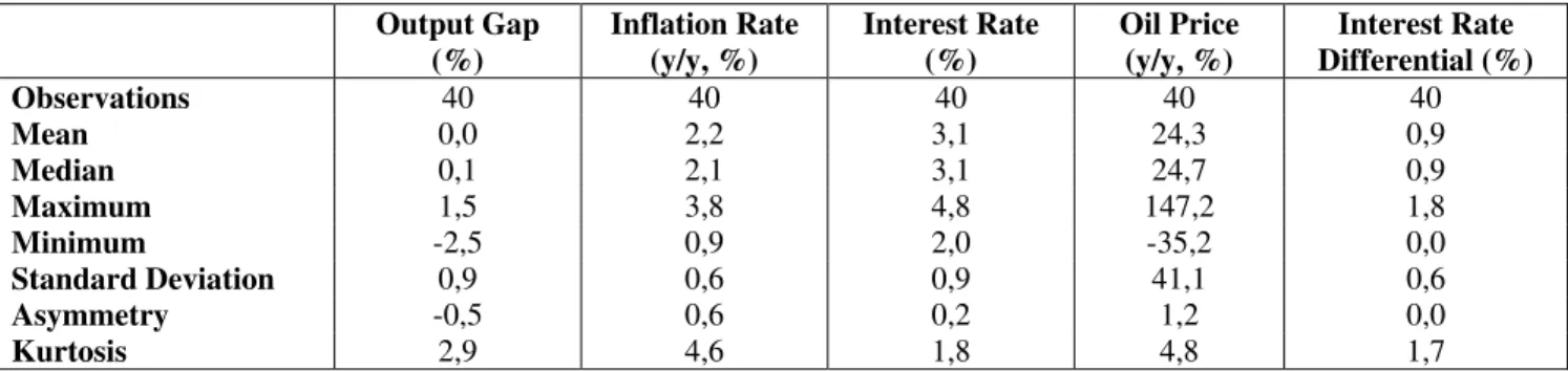
In addition to the core variables of the NKM (output gap, inflation rate and interest rate), we use another two variables (oil price and interest rate differential) as part of our instrument set. Table 5 contains some descriptive statistics of the data.
Finally, we assume the stationarity of all data, a property that is assumed to be valid in most theoretical and empirical studies of this nature, as underlined by Clarida et al. (1998). In fact, Clarida
et al. (1998) emphasise that the most usual unit root tests (Augmented Dickey–Fuller test, Phillips–
Perron test and Kwiatkowski–Phillips–Schmidt–Shin test) are sensitive to sample size and have very
low power in small samples. Thus, its application to the variables herein could lead to counterproductive results, because the sample includes only 40 observations.
Table 5: The descriptive statistics of the data
Output Gap (%) Inflation Rate (y/y, %) Interest Rate (%) Oil Price (y/y, %) Interest Rate Differential (%) Observations 40 40 40 40 40 Mean 0,0 2,2 3,1 24,3 0,9 Median 0,1 2,1 3,1 24,7 0,9 Maximum 1,5 3,8 4,8 147,2 1,8 Minimum -2,5 0,9 2,0 -35,2 0,0 Standard Deviation 0,9 0,6 0,9 41,1 0,6 Asymmetry -0,5 0,6 0,2 1,2 0,0 Kurtosis 2,9 4,6 1,8 4,8 1,7
3.2.1. The Output Gap
The output gap is the difference between GDP and the respective long-term trend (potential GDP). We started to collect the GDP for the euro area (at 2000 market prices, millions of euro, seasonally
adjusted and changing composition) and then applied the Hodrick–Prescott (1997) filter, using a smoothing parameter of 16008 to obtain the respective trend. McMorrow and Roeger (2001) noted,
besides being a judgement-free method, that it seems to adapt relatively well to the evolution of economic activity in the euro area. At the same time, they show that other methods present similar results, although data obtained from the Hodrick–Prescott filter present less volatility. Finally, we obtained the output gap by deducting the respective trend from the log GDP.
3.2.2. The Inflation Rate
We use the annual inflation rate measured by the HIPC in the euro area (seasonally adjusted and changing composition), since this is the preferred measure of the ECB to monitor the evolution of general prices in the euro area. The quarterly inflation rate was calculated by the average of the annual inflation rates observed in each month of the respective quarter.
3.2.3. The Interest Rate
The interest rate chosen corresponds to the main key interest rate decided by the ECB in its monthly monetary policy meetings, namely the rate of main refinancing operations (known as the refi rate). The quarterly interest rate was calculated by the average of the interest rate fixed in each monthly monetary policy meeting.
3.2.4. The Oil Price
We use the oil price of a brent barrel (in euros), which is the oil produced in the North Sea and acts as a reference for the derivatives market in Europe and Asia. Then, we calculated the quarterly average of the respective oil prices and after we calculated the respective annual rates (at current prices).
3.2.5. The Interest Rate Differential
The interest rate differential used here came from the difference between the yields of German government 10-year bonds (known as bunds) and those of two years (known as schatz), since the bonds issued by the German government serve as a reference for the euro area. We use the quarterly average of the respective differential on each day.
4. Empirical Results: Main Remarks
The IS Curve, Phillips Curve and Taylor Rule were estimated individually through the GMM. To fulfil this purpose, the expected variables in the future (unknown variables) are replaced by their ex post values. Five lags of the output gap, the inflation rate, the interest rate, the oil price and the interest rate differential were used as a set of instruments, which is quite similar to the set of instruments used by Galí and Gertler (1999) or Clarida et al. (2000) for the US economy and Galí et al. (2001) for the European economy.
4.1. The is Curve
Under the assumption of rational expectations, the expectations unobserved and based on the
information in period t could be eliminated; thus, the set of orthogonality conditions implicit in the IS Curve can be presented as:
8 There are no indications in economic theory of the ideal value for capturing this trend. However, in practice there is a certain “unanimity” to λ by assuming a value at 14,400 for monthly data, 1600 for quarterly data and 100 for annual data, as pointed out by Sørensen and Whitta-Jacobsen (2005).
[
]
{
t+ t − t+1 − t+1− t−1 t}
=0t x (i π ) μx δx z
E ϕ (48)
The orthogonality condition forms the basis of estimating the IS Curve via the GMM, as shown in Table 6.
Table 6: Estimates of the IS Curve
φ µ δ
Coefficient 0,10 0,31 0,58
Standard Error (0,01) (0,01) (0,02)
P-value 0 0 0
J-statistic 0,62
P-value Wald test (µ+δ=1) 0
Observations 40
First, note that the observed value of J-statistic (0.62) is clearly less than the critical value of the chi-square distribution with 22 degrees of freedom at a level of trust of 95% (33.9). Thus, the set of orthogonality conditions cannot be rejected and, therefore, the specification of the model is accepted and the set of instruments is valid.
All parameters are statistically significant and hold the expected signs, in a context where the real interest rate is the variable that influences the output gap in the euro area to a lesser degree. As stated by Djoudad and Gauthier (2003), this result is common in the literature. They argue that “the
traditional interest rate channel seems controversial, as Bernanke and Gertler (1995) point out: empirical studies have great difficulty in identifying significant interest rate effects on output, perhaps because monetary policy operates through other channels (e.g., asset prices, exchange rate, credit,
wealth effect) than the short-term interest rate” (Djoudad and Gauthier, 2003, p. 12).
The counterintuitive (positive) effect of the real interest rate on the product (IS puzzle) is not verified, which indicates that there are no omitted significant variables in the IS Curve estimation for the euro area economy, as pointed by Goodhart and Hofmann (2005). In this regard, governments in the euro area should aim for a more active stance in their fiscal and budgetary policies, in a context where monetary policy stimulus seems to be less relevant to the evolution of aggregate demand. This requires a higher fiscal discipline by all governments in order to always achieve a margin of manoeuvre to adopt expansionary policies without worrying about the sustainability of public finances or the accumulation of excessive deficit, even in recessionary economic periods.
By contrast, the evolution of the lagged output gap has a higher explanatory power in the current output gap than the expected future output gap, which suggests that output in the euro area shows a certain persistence and, consequently, that business cycles may be longer and lasting. This illustrates the reason why recessions are so feared by the ECB and other authorities in the euro area. Further, the IS Curve could constitute a useful tool to describe aggregate demand in the euro area, in a context where the correlation between the output gap the IS Curve estimation is strong, as demonstrated in
Figure 1: The effective output gap and the estimated Is Curve
Note that the sum of estimated coefficients that measures the variations in expected future output and lagged output in current output is nearly equal to unity, namely µ∧+δ∧ =0,89, although the a Wald test (test of the restriction of parameters) rejects the inference of this hypothesis. Indeed, the hybrid version of the IS Curve seems to denote a higher explanatory power in the description of aggregate demand in the euro area than the canonical version.
Finally, the backward looking component clearly supplants the forward looking component in the explanation of the behaviour of aggregate demand in the euro area, which is in line with the findings obtained by Fuhrer and Rudebush (2004) for the US economy in the period between the first quarter of 1966 and the last quarter of 2000.
4.2. The Phillips Curve
Under the assumption of rational expectations, unobserved expectations based on the information in period t could be eliminated, and thus the set of orthogonality conditions implicit in the reduced form of the Phillips Curve can be described as:
[
]
{
t − t − t+1− t−1 t}
=0t π λx απ γπ z
E (49)
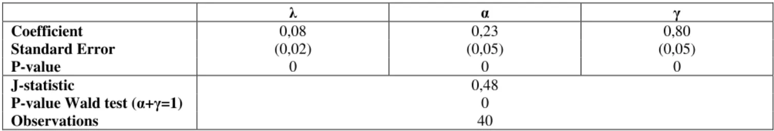
The orthogonality condition forms the basis to estimate the reduced form of the Phillips Curve via the GMM (Table 7).
Table 7: Estimates of the reduced form of the Phillips Curve
λ α γ
Coefficient 0,08 0,23 0,80
Standard Error (0,02) (0,05) (0,05)
P-value 0 0 0
J-statistic 0,48
P-value Wald test (α+γ=1) 0
Observations 40
Firstly, the observed J-statistic value (0.48) is clearly less than the critical value of the chi-square distribution with 22 degrees of freedom at a level of trust of 95% (33.9), so the orthogonality conditions cannot be rejected, namely the validity of the used instruments in the estimation and specification of the model is accepted.
Once again, all parameters are statistically significant and hold the expected signs. The variable that influence current inflation rate evolution in the euro area to a lesser degree is output gap, although there is no counterintuitive (negative) effect of the output gap over the inflation rate (see Galí and
-1,2 -0,8 -0,4 0,0 0,4 0,8 1,2 1,6 -1,2 -0,8 -0,4 0,0 0,4 0,8 1,2 1,6 Ju n-00 Ju n-01 Ju n-02 Ju n-03 Ju n-04 Ju n-05 Ju n-06 Ju n-07 Ju n-08
Gertler, 1999; Galí et al., 2001). So, the output gap could be a driver for the inflation rate in the euro area, contrary to what happens in the US (Galí and Gertler, 1999).
Moreover, no distribution is clearly equitable between the backward looking and forward looking components, as the lagged inflation rate influences the current inflation rate more than the expected future inflation rate. As such, the inflation rate in the euro zone denotes a higher degree of viscosity, which appeals to the need to avoid strongly inflationary and/or deflationary economic contexts, which could become extended and durable. This high degree of persistence in the euro area inflation rate may essentially derive from the strong rigidity of the respective labour markets, which contrast with the higher flexibility in the US economy, as emphasised by Fabiani and Rodriguez-Palenzuela (2001). Perhaps for this reason, the ECB displays an irreducible attitude in its goals by maintaining the inflation rate below, but close to 2% in the medium term, since any deviation may prove to be prolonged, jeopardising a favourable economic environment and sustainable growth.
These results also suggest that the reduced form of the Phillips Curve describes reasonably well the evolution of the inflation rate in the euro area. This is so even though other factors may be equally responsible by its evolution over time (e.g., the evolution of monetary policy by itself and/or the existence of supply shocks), since the correlation between the inflation rate and estimation of the reduced form of the Phillips Curve is weaker than the case of the IS Curve (Figure 2).
Figure 2: The effective inflation rate and the estimated reduced form of the Phillips Curve
Additionally, the sum of the estimated coefficients, which measures the variations in the expected future inflation rate and the lagged inflation rate in the current inflation rate, is nearly equal to unity, namely α∧+γ∧=1,03; however, the Wald test rejects this hypothesis. Therefore, the hybrid version of the reduced form of the Phillips Curve seems to denote a higher explanatory power in the description of inflation rate behaviour in the euro area than the purely canonical version.
Similar to what happens with the IS Curve estimation, the backward looking component clearly supplants the forward looking component, which is closer to the conclusions obtained by Fuhrer and Moorer (1995) and McAdam and Willman (2003) for the European economy than those of Galí and Gertler (1999) for the US economy and Galí et al. (2001) for the European economy, which emphasise the forward looking component in the explanation of the inflation rate.
Regarding the structural form of the Phillips Curve, and under the assumption of rational expectations, non-observed expectations based on the information in period t could be eliminated, and thus the set of orthogonality conditions could have the following structure:
[
]
{
(1 )(1 )(1 )}
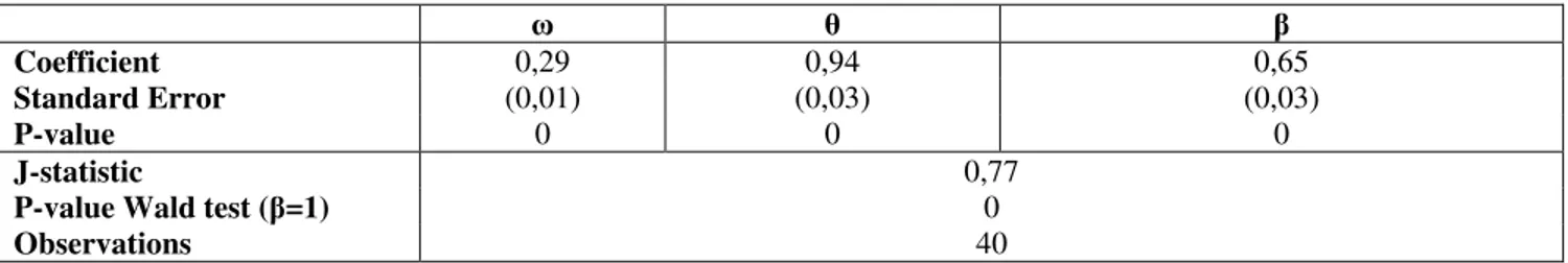
0 E 1 1 1 1 1 t t − − − − − − − = − + − − t t t t z x βθφ π ωφ π φ βθ θ ω π (50)The orthogonality condition represents the basis to estimate the structural form of the Phillips Curve using the GMM (
Table 8). 1,5 2,0 2,5 3,0 3,5 4,0 1,5 2,0 2,5 3,0 3,5 4,0 Ju n-00 Ju n-01 Ju n-02 Ju n-03 Ju n-04 Ju n-05 Ju n-06 Ju n-07 Ju n-08