1Optics Laboratories, P.O. Box 1021, Islamabad, Pakistan
2Instituto de Física de São Carlos, Universidade de São Paulo, Caixa Postal 369, 13560-970 São Carlos, SP, Brasil 3Université Paul Sabatier, 118 route de Narbonne, 31062 Toulouse, France
Manuscript received on July 7, 2007; accepted for publication on December 18, 2007; contributed byVANDERLEIS. BAGNATO*
ABSTRACT
Cesium atomic beam clocks have been the workhorse for many demanding applications in science and technology for the past four decades. Tests of the fundamental laws of physics and the search for minute changes in fundamental constants, the synchronization of telecommunication networks, and realization of the satellite-based global positioning system would not be possible without atomic clocks. The adoption of optical cooling and trapping techniques, has produced a major advance in atomic clock precision. Cold-atom fountain and compact cold-Cold-atom clocks have also been developed. Measurement precision of a few parts in 1015has been demonstrated for a cold-atom fountain clock. We present here an overview of the
time and frequency metrology program based on cesium atoms under development at USP São Carlos. This activity consists of construction and characterization of atomic-beam, and several variations of cold-atom clocks. We discuss the basic working principles, construction, evaluation, and important applications of atomic clocks in the Brazilian program.
Key words:atomic clock, cold atoms, time and frequency, metrology.
INTRODUCTION
Precise measurement of time and frequency has great importance in commercial and defense applications as well as in fundamental physics. Each atom or molecule absorbs and emits electromagnetic radiation at characteristic transition frequencies. Some of these frequencies lend themselves to stabilization over time and space and therefore constitute natural frequency standards. The U.S. National Institute for Standard and Technology (NIST) built up its first frequency standard clock based upon an ammonia transition in 1949 (Lyons 1949). The ammonia clock performance, however, was not better than conventional clocks existing at that time. The National Physical Laboratory (NPL) in England built up the first practical cesium
atomic clock in 1955 (Essen and Parry 1957), and in 1967 atomic clock technology enabled scientists to define the unit of time, the second, based on atomic measurements (CGPM 1967).
In current primary atomic frequency standards, transitions between ground state hyperfine energy levels in cesium atoms at microwave frequencies form the basis for measuring time. The present definition is: The second is the duration of 9 192 631 770 periods of the radiation corresponding to the transition between the two hyperfine levels of the ground state of the cesium 133 atom at a temperature of 0 K.
1 second=9 192 631 770 periods of the Cs133, F =3, mF =0↔F =4, mF =0 hyperfine transition
The usual stability (precision) of Cs atomic beam clocks is a few parts in 1013, and the uncertainty (accuracy)
is of the order of one part in 1014. For the modern cold-atom fountain clock two orders of improvement in
stability is possible and about one order in uncertainty. Atomic clocks use natural internal-state transitions within atoms or molecules to keep time. These quantum mechanical oscillators are vastly less sensitive to gross environmental effects such as temperature, pressure, humidity, and vibration, for example, than macroscopic oscillators such as pendulums and quartz crystals. But the most important advantage of atomic clocks is that every atom of a given element and isotope is identical. Therefore an atomic clock standard based on Cs133transitions is transferable the world over. The atomic clock is the most stable and accurate
clock known. Atomic clocks are so good that time and frequency can be measured more precisely than any other physical quantity. Cesium atomic clocks are the primary standard, and rubidium clocks are accepted as a secondary standard.
Modern life depends upon the precise time. Communication, financial transactions, electric power and many other activities have become dependent upon time accuracy. The demand of these technologies will continue to drive research toward more accurate, precise, and transferable time standards. Improvement in the development of the frequency and time standard is continually in progress. Development of the harmonic generating “frequency comb” made the optical frequency regime a prominent candidate for an advanced frequency standard. Cold atoms and cold ions are certainly the most promising systems for the development of a new atomic standard (Bize et al. 2005, Ma et al. 2004, Udem et al. 2002). Any country which aspires to develop and grow technologically must include a serious program ofscientifictime and
frequency metrology.
The official Brazilian time scale is maintained by the Observatório Nacional, located in Rio de Janeiro and associated with the Brazilian institute of metrology, Instituto Nacional de Metrologia, Nomalização e Qualidade Industrial (INMETRO). This service is implemented with commercial cesium and rubidium clocks. In this paper we provide an overview of the scientific time and frequency program at University of São Paulo in São Carlos. The program is composed of different types of atomic clocks based on cesium atoms. Historically the earth’s rotation was used as a time standard, and we start by discussing how this standard relates to the atomic standard. We then discuss briefly some of the current applications for atomic clocks followed by a more detailed description of clocks constructed and under development at USP São Carlos.
SYSTEMS OF TIME: UTC AND TAI
from atomic standardswith no reference to the rotation of the Earth. At any particular time, UTC proceeds
as a linear function of TAI, and since 1972 UTC “ticks” at the same rate as TAI. UTC occasionally has discontinuities where it changes from one linear function of TAI to another. These discontinuities take the form of leaps implemented by a UTC day of irregular length. The accuracy and stability of atomic clocks is the effective standard for TAI. Atomic clocks maintain a continuous and stable time scale for TAI, and provide an excellent reference for time and frequency in scientific applications. The UTC, not the TAI, is the time distributed by standard radio stations that broadcast time, such as WWV and WWVH. It can also be obtained readily from the GPS satellites (Audoin and Guinot 2001, Nelson et al. 2001, Riehle 2004, Jesperson and Fitz-Randolph 1999).
APPLICATIONS OF ATOMIC STANDARDS
The precise and accurate measurement of time and frequency plays a fundamental and important role in the success of many fields of technologies and research. Atomic clock technology has several practical applications. On the scientific side, atomic clocks provide a sensitive probe for minute variations in physical constants such as the fine structure constant, α. Clocks can also be used to search for variations in the
isotropy of space, preferred frames of reference, charge- parity-time (CPT) symmetry violation and to test the theories of relativity and electrodynamics (Uzan 2003). Precise and accurate clocks may provide the means to revel new phenomena signaling a fundamental change in how we perceive nature (Riehle 2004, Audoin and Guinot 2001). Practical applications include metrology, geodesy, global positioning systems for navigation, communication, electric power networks and defense. We shall briefly discuss these practical applications as well.
FUNDAMENTALPHYSICS RESEARCH
According to Einstein’s Equivalence Principle (Vessot and Levine 1979), fundamental constants should not vary with time, but some modern theories predict the existence of variation. The development of atomic clocks (Cs and Rb) have provided the accuracy necessary to test fundamental constants like the Rydberg constant R and the fine structure constantαand their possible slow variation with respect to time. Recently
frequencies in Rb and Cs atoms. d dt ln νRb νCs = µRb µCs
α−0.44=(0.2±7.0)×10−16year−1 (1)
whereµRbandµCsare the magnetic moments of rubidium and cesium respectively. Furthermore it can be shown that the sensitivity of the ratio ofνRb/νCsto a variation ofαis given by
∂ ∂lnαln
νRb
νCs
≃ −0.44 (2)
Combining Eqs. 1 and 2, the upper limit to the fractional time variation of the fine structure constant is
˙ α
α =(−0.4±16)×10
−16 yr−1 (3)
(Marion et al. 2003). In another approach (Peik et al. 2004) measured an optical transition frequency in the Yb+ ion over a period of almost three years and were able to relate the constancy of this frequency to an upper limit on the variability of α of 2.0×10⁻¹⁵ yr−1. The advantage of this approach is that it is
independent of the assumed constancy of the atomic masses or magnetic moments.
Precise atomic spectroscopy, precision interferometry for gravitational wave detection, and other as-trophysical measurements as well as tests for relativity, quantum electrodynamics and CPT invariance can be made possible using ultra-stable atomic clocks (Bize et al. 2005, Flambaum and Tedesco 2006, Uzan 2003, Vessot et al. 1980).
In 1993 the quantitygp(me/mp)was measured by comparing the frequency data of Cs and Mg atomic beam standards (Godone et al. 1993), wheregpis the proton gyromagnetic ratio andme,mpare the mass of the electron and proton respectively. The time stability of this quantity is an important subject for theoretical physics as well as for dimensional metrology. The study of time variation of such quantities or its product with fine structure constant plays an important role in definition of international standards (SI).
We list here a few specific examples of important applications in time and frequency measurements.
Time dilation test
U.S. Naval Observatory performed an experiment to test time dilation in 1971, (Hafele and Keating 1972). Airline flights around the world in opposite directions carried four Cs atomic beam clocks. At the end of the flights it was found that the traveling clocks gained about 0.15µs relative to rest clocks. Measurement
of time dilation has been an important test for special relativity.
Pulsar frequency detection
navigate using GPS although it is not yet acceptable to land an aircraft by GPS alone since atomic clocks on satellites are still not accurate enough and it takes too long to compute positions. These atomic clocks are periodically updated from the ground primary Cs clock at the U.S. Naval Observatory. These satellites transmit both timing and positioning data. The combination of primary frequency standard (Cs atomic clock) and commercial atomic standards (Cs and Rb clocks) and a stable communication network provide accurate time and frequency. The GPS provides altitude, latitude and longitude with an uncertainty of less than 10 meters. Improvement in the ground-based master clocks that calibrate the GPS atomic clocks along with better satellite clocks will allow transportation systems to locate vehicles with sub-meter precision in real time. It is not only the GPS space system that carries atomic clocks on board. The Russian navigation satellite system, Glonass, is also similarly equipped. Initially implemented in the Soviet Union, this system fell into disrepair, but with the help of the Indian government it is now being restored. Other proposed systems are in development such as COMPASS (China), GALILEO (European Union), and an updated version of GPS called GPS III that is planned to be fully operational in 2013. Communication satellite systems such as Milstar require the robust timekeeping capabilities of atomic clocks in order to provide secure communications. As the competition for radio frequency bandwidth increases, other communication systems, commercial as well as military, may have to rely on atomic clocks to provide accurate frequency and time on board spacecraft. Satellite ranging for deep space will require an accuracy of 1015 to 1017,
(Allan et al. 1994, Audoin and Guinot 2001, Bauch 2003, McCaskill et al. 1999, Riehle 2004, Wu and Feess 2000).
SPACEGEODESY
LENGTH ANDOTHERPHYSICAL PROPERTIESMEASURED ASFREQUENCY
Presently there exists no other quantity measured as precisely as frequency. Due to this unique capability, it is possible to measure more precisely other physical quantities using frequency and time. Considerable efforts are under way to translate the measurement of length, speed, temperature, electric field, magnetic field, voltage, etc. into frequency. The meter (m) is the Système International (SI) unit of length and is now defined as the length of the path traveled by light in vacuum during the time interval of 1/299 792 458 of a second, i.e. 1/c. This new definition replaces two previous definitions of the meter: the original adopted in 1889 based on a platinum-iridium prototype bar, and a definition adopted in 1960 based on a krypton-86 radiation from an electrical discharge lamp. The krypton-86 electrical discharge lamp was designed to produce the Doppler-broadened wavelength of the 2p10-5d5 transition of the unperturbed atom. The two dominant wavelength shifts, one caused by the DC Stark effect and the other by the gas pressure in the discharge lamp, were opposite in sign and could be made equal in magnitude by the proper choice of operating conditions. Different krypton-86 lamps reproduced the same wavelength to about 4 parts in 109, but had the disadvantage that the coherence length of its radiation was shorter than the meter,
complicating the changeover from the older standard. Faced with the possibility that further advances in laser spectroscopy would lead to proposals for new length standards based on more precise atoms or molecules, a new concept for the length standard definition was developed. The second (which is equivalent to 9,129,631,770 oscillations of the cesium-133 microwave transition) and the meter are now considered independent base units. Traditionally, the speed of light was measured in terms of their ratio. By contrast, the present standard defines the meter in terms of the SI second and adefinedvalue for the speed of light in
vacuum which fixes it to 299 792 458 m s−1exactly. Thus the meter is determined experimentally based on
the cesium-133 frequency standard. Since it is not based on a particular radiation, this definition opens the way to major improvements in the precision with which the meter can be realized using laser techniques without redefining the length standard. As a practical matter the meter can be measured at different, more convenient optical frequencies and referenced back to the cesium-133 standard using frequency chains (Udem et al. 2002).
TIMESYNCHRONIZATION OFCOMPUTERS
The discussion in the section is taken from the Wikipedia entry on the Network Time Protocol. The Network Time Protocol (NTP) is a protocol for synchronizing the clocks of computer systems over packet-switched, variable-latency data networks. NTP uses an algorithm with the UTC time scale, including support for features such as leap seconds. NTP v4 can usually maintain time to within 10 milliseconds (1/100 s) over the public Internet, and can achieve accuracies of 200 microseconds (1/5000 s) or better in local area networks under ideal conditions. Atomic clocks are used to synchronize computer clocks. NTP uses a hierarchical system of “clock strata”. The stratum levels define the distance from the reference clock and the associated accuracy.
Stratum 0
reference a number of Stratum 1 servers and use the NTP algorithm to gather the best data sample, dropping any Stratum 1 servers that seem obviously wrong. Stratum 2 computers will peer with other Stratum 2 computers to provide more stable and robust time for all devices in the peer group. Stratum 2 computers normally act as servers for Stratum 3 NTP requests.
Stratum 3
These computers employ exactly the same NTP functions of peering and data sampling as Stratum 2, and can themselves act as servers for higher strata, potentially up to 16 levels. NTP (depending on what version of NTP protocol in use) supports up to 256 strata. It is hoped that in NTP 5 (a protocol still in development) that only 8 or 16 strata will be permitted.
DEFENSE
Frequency standards and clocks play a major role in military communication, navigation, surveillance, missile guidance, Identification Friend or Foe (IFF) and Electronic Warfare (EW) systems. The major enabling technologies require robustness to environmental disturbances, low input power, long stability, high accuracy, small size and weight. Development of more compact atomic clocks will better meet these requirements. The mobility and robustness of military systems and platforms can be improved by using ultra-miniature time reference units such as chip-scale atomic clocks. The ultra-stable frequency reference provided by atomic clocks will drastically improve channel selectivity and density for all military communications.
IMPLEMENTATION OF ATOMIC FREQUENCY STANDARDS
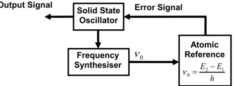
Atomic frequency standard can be either active or passive. An active atomic standard uses the electromag-netic radiation emitted by atoms themselves as they decay from a higher energy state to a lower energy state. A passive standard matches the frequency of an electronic oscillator or laser to the resonant frequency of the atoms by means of a feedback circuit.
operation. This transition frequency is intrinsically independent of space and time. When an electronic transition takes place in the atom between two energy levels, it either emits or absorbs an electromagnetic (EM) wave with a center frequencyν0.
Fig. 1 – Schematic diagram showing the working principle of the atomic clock.
All the atoms of the same element and isotope absorb or emit electromagnetic radiation of the same frequency. This is the fundamental difference of atomic clocks as compared to other time-keeping devices. The microwave oscillator provides the frequency for the atomic transition which, through the atoms, is corrected until the difference between the frequency of the oscillator and the atoms is minimized. The oscillator is then locked to this transition using a feed back loop. The choice of a specific frequency of a selected atom depends on certain requirements to acquire best accuracy and stability. To obtain high precision, the natural line width of the transition should be as small as possible and the interaction time between the atomic and radiation should be as long as possible. This characteristic implies a high quality factorQ =ν0/ν0for the atomic transition. Signal to noise ratio (S/N) of the observed resonance transition
should be large to minimize statistical fluctuations of the signal controlling the local oscillator (LO). The velocity of the atoms should be low to minimize Doppler shifts. The resonance atomic transition should be insensitive to electric and magnetic fields and to pressure broadening effects.
How to measure the clock transition with minimum external influence?
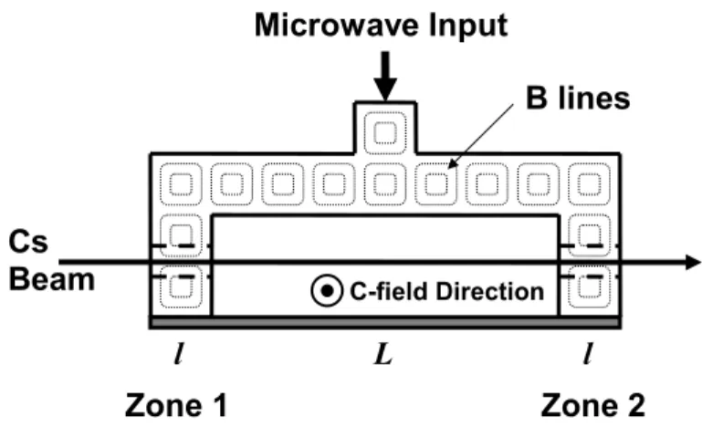
An ingenious answer to this key question is the idea of Ramsey (Ramsey 1950) known as the two-separated-zones interaction in an atomic beam. In this method, when the atom beam travels down an evacuated tube, the atoms interact with two separated microwave cavities. The probability that an atomic transition in the first and in the second zone occurs depends upon a number of parameters.
RAMSEYMETHOD
In the Ramsey method, atoms in the beam pass through two separated zones of lengthlhaving two
phase-coherent microwave fields that are spatially separated by the distanceL, whereL >>l. The characteristic
Fig. 2 – Schematic diagram of the Ramsey two-zone atomic beam clock.
To understand how the Ramsey technique reduces the line width of a transition, consider a two-level atom with states|0and|1. At time t =0, this atom enters a microwave region of lengthl, where it is
perturbed by an oscillatory microwave electromagnetic field and as a result an atomic excitation takes place. The probabilityP of transition between the two states|0and|1is given by the following equation.
P(τ )= b 2
2sin 2τ
2
with
=(ω0−ω)2+b2 1/2
and b= µB
B
Hereτ is the interaction time within the zonel,ω0is the atomic transition frequency,ωis the applied
microwave frequency,µB is the Bohr magneton, B is the amplitude of the microwave magnetic field and
is Planck’s constant divided by 2π. The quantity b is a measure of the strength of the magnetic dipole
coupling between the magnetic component of the microwave field and the atom. It is known as the Rabi frequency (Ramsey 1990). The first factor on the right hand side of the expression for P(τ ) becomes
unity whenω=ω0(resonance) and the full width at half maximum isω = 5.02/τ. The second factor
is time-dependent. The probability will be maximum atω = ω0, whenbτ =π. The interaction time is τ =l/υwhereυis the velocity of the atomic beam andlis the length of interaction region. The width for
such a transition under these conditions can be expressed asω=5.02/τ =5.02υ/l.
The above equation implies that the transitions can be made arbitrarily narrow as the length of the interaction zone is increased. However, in practice this cannot be realized due to two limitations: loss of beam intensity and the impossibility to achieve homogenous B-field amplitude throughout the interaction zone. The resonance frequency will differ along the beam path and resulting in broader resonances instead of narrower. Ramsey’s ingenious idea of two separated fields not only overcomes the problem of field inho-mogeneity but in addition generates resonances much narrower than those arising from a single interaction. The transition probability in the case of the two-zone Ramsey configuration is calculated from the following equation.
P(τ,T, ,b)=4b
2
2sin 2τ
2 × cosτ 2 cos
0T +ϕ
2 −
0
sin
τ
2 sin
0T +ϕ
2 2
Hereϕ is the phase shift andT is the duration of the time interval between the two separated interaction
zones.
In the on-resonance case, all of the atoms will undergo transition resulting in maximum signal. Now if the frequency is slightly off resonance, there will be a difference in the phase of the atomic states between the first and second interaction zones, and some of the atoms will be left in the original atomic state. The signal will decrease. In case of one half of the phase difference, none of the atoms will make the transition and the signal will be minimum. If the phase difference is complete integral multiple of cycle then we will observe other maxima signal and in case of half integral multiple phase difference, we will observe other a minima.
The probability will be maximum when ϕ = 0, 0 = 0 and bτ = π/2. For0 = 0 the motion
of the atoms in field free region produces interference effects. The generation of interference fringes is called a Ramsey pattern. The interference pattern arises because of the two separated interrogation regions (Ramsey 1950, 1963, 1990).
The central fringe has the principal importance of providing the atomic frequency reference. Its peak-to-valley height is taken as the amplitude of the resonance profile. The full width at half maximum (FWHM) given as
FWHM=ν ∼= π T =π
υ L
HereL is separation between two interaction zones. As a numerical example considerυ =200 ms−1and L =10 cm, ν=6.283 KHz. Asbτ =π/2→, b =31400 rad s−1forl=1 cm, (interaction region).
Hence the corresponding amplitude of the microwave magnetic field B=0.357µT.
Two extreme cases can be considered separately: The central feature of the Ramsey fringe,0<<b
and the “Rabi Pedestal”,0>>b(Ramsey 1963, Vanier and Audoin 1989).
For0<<b
P(τ )= 1
2
1+cos(0T +ϕ)sin2(bτ ) . (5)
For0>>b
P(τ )= 1
2
b2 2
sin2(τ )+0
(1−cos(τ ))
2
.
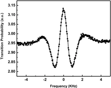
Figure 3 illustrates the recorded signal of the Ramsey central fringe and Figure 4 all seven possible Zeeman transitions 6S1/2(F =3)→6S1/2(F =4);mF =0. The signal consists of a narrow spectral feature (Ramsey central fringe) superimposed on the broader envelope(Rabi pedestal). The Rabi pedestal is related to the transit time broadening as the atoms pass through the two microwave regions as well as the velocity distribution of the atoms in the thermal beam. This pedestal is much more significant for the atomic-beam frequency standard (20 kHz) than for the atomic fountain (cf. Section 6) using optically cooled atoms (70 Hz). The overall shape of the Rabi pedestal is due to the combined effects of the probability that a transition occurs in the first excitation region but not in the second, plus the probability that it occurs in the second excitation zone but not in the first.
Fig. 3 – Ramsey interference pattern showing central fringe and broad Rabi pedestal.
Fig. 4 – The seven Zeeman sublevel transitions possible for the 6S1/2(F=3)→6S1/2(F =4);mF=0.
CESIUM BEAM ATOMIC CLOCK
The cesium atom has proved to be a good choice for the development of a clock. Three kinds of cesium clocks are under development in Brazil. These are the cesium atomic beam, the cesium fountain and the cesium “expanding cold atoms” clock. All of these cesium-based atomic clocks have been constructed and evaluated at the University of São Paulo at São Carlos.
The Cs133 atom is a stable element. It is highly electropositive and reactive. The saturating Cs vapor
pressure at room temperature and at 100◦C is 1.86×10⁻⁴and 7.45×10⁻²Pa, respectively. Cesium has only
one valence electron and a2S
1/2ground-state Russell-Saunders term. The nuclear magnetic spin of Cs133
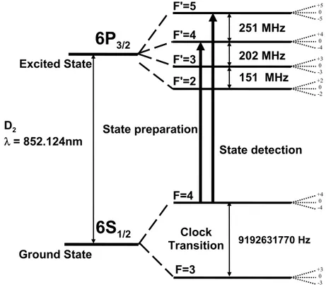
the two hyperfine levels are populated according to their 2F +1 degeneracies. Figure 5 illustrates the
relevant term energy diagram of Cs133. The energy of the Zeeman sublevels, labeledm
F, is proportional to the applied magnetic field and is expressed in units of kHz/G. In the absence of an external magnetic field, themF Zeeman sublevels are degenerate.
Fig. 5 – Diagram of the internal levels and transitions relevant to the Cs atomic beam clock.
The clock transition between between states F =3, mF =0 to F =4, mF =0 is a magnetic dipole transition. The probability of spontaneous magnetic dipole relaxation from the upper hyperfine state is very low, and therefore atoms in the excited stateF = 4, mF = 0 will remain there for a very long time compared to the observation time.
CONSTRUCTION OF THECESIUMATOMICBEAMCLOCK
The Brazilian Cs atomic beam clock was designed and developed following the scheme of the Ramsey two-separated-microwave- interaction zones. The basic advantage of this experimental scheme is the reduction of time-of-flight broadening and increase of the atoms number that participates during the interrogation and detection process. The natural line width of radio frequency and microwave transitions is extremely small because the spontaneous transition probability is proportional to the frequency cubed. Therefore, the spectral line width of these transitions is determined by transit-time broadeningν =1/T = υ/L. The
termT is the atom time of flight between two microwave interaction zones,υis the velocity of the atoms
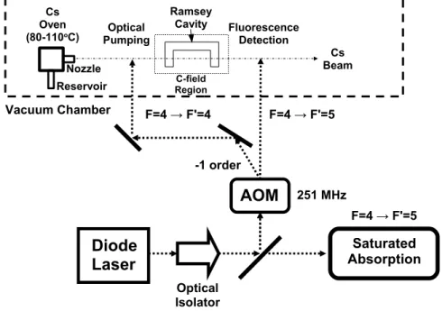
Fig. 6 – Schematic diagram of the Cs atomic beam clock.
The C-field is produced by using four coils as illustrated in Figure 6. This configuration produces a magnetic field perpendicular to the atomic beam and is used to lift the degeneracy of the hyperfine sublevels
mF of the Cs ground state. The U-shaped copper microwave cavity consists of two interrogation zones, each having 10 mm length and 5 mm width. The separation between the two zones is 90 mm. The atoms in the two zones interact with microwaves generated by the microwave synthesizer. The quality factor
Q(= ν/ν)of the cavity is about 500 at the oscillation frequency of 9.2 GHz. The whole microwave
cavity region is shielded withµmetal to avoid external magnetic field perturbations.
The Cs atoms are prepared in a selected ground state hyperfine level and detected using laser induced fluorescence before and after the microwave cavity region using a stabilized diode laser (Teles et al. 2000).
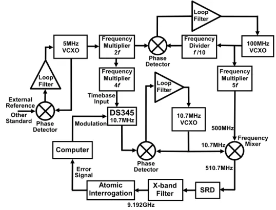
Microwave synthesizer, control and comparison
constituted of three base high performance quartz oscillators (5 MHz, 100 MHz and 10.7 MHz Wenzell VCXO’s). Phase Locked Loops (Phase Detectors and Loops Filters) are implemented in order to extract the best spectral characteristics of each oscillator and synthesize the 9.192 GHz interrogation signal. An external DDS (Direct Digital Synthesizer – SR345 Stanford), driven in external reference by the 5 MHz oscillator, provides the capability to sweep the microwave signal. Once phase locked to the 5 MHz oscillator, the 100 MHz signal is multiplied by a factor of five. The 500 MHz signal is then mixed to the signal from the 10.7 MHz oscillator and feeds a Step Recovery Diode (SRD). This device, based on a nonlinear effect, generates a frequency comb with the harmonics of the 510.7 MHz input signal. With proper filtering, only the 18th harmonic of 510.7 MHz is obtained, producing 9.1926 GHz. The 10.7 MHz oscillator is phase locked to the external DDS, in order to provide a fine-tuning capability in the microwave signal. A LabVIEW computer interface program controls the DDS. The synthesizer has the frequency resolution of 18×10−6Hz and fractional frequency stability better than 3×10⁻¹⁴τ−1/2for 104seconds of averaging
time.
Fig. 7 – Schematic diagram of the microwave synthesizer for the beam clock.
Optical pumping and detection
was locked at the 62S
1/2(F = 4) −→ 62P3/2(F = 5)transition of the saturation absorption line of the
cesium cell to avoid the long term drift. The remaining part of the laser beam was propagated through the acoustic optical modulator (AOM). The AOM modulator was operated at 250 MHz to generate first order diffracted and zero order beams for pumping 62S
1/2(F = 4) −→ 62P3/2(F = 4) and detection
62S
1/2(F = 4) −→ 62P3/2(F = 5) respectively (Teles et al. 2000). Optical pumping for the radiative
transitions in alkalies takes about 10µsec.
EVALUATION OF THECS ATOMICBEAMCLOCK
The performance of a time and frequency standards depends on stability, frequency shifts uncertainty and accuracy. The stability criterion can be divided into short and long term stability, both of which are evaluated by the “Allan variance”. The frequency shift of true hyperfine transitions can occur due to a number of external and internal perturbations such as black body transitions, Gravitational field, and Doppler and Zeeman effects. These effects manifest themselves as frequency offsets.
Before presenting the clock evaluation, it is worthwhile to introduce the concepts of accuracy, stability, and reproducibility. They are often used to describe an atomic clock quality with respect to its instabilities.
Accuracyis the degree of correctness of a quantity with respect to the true value. It is related to the offset from an ideal value. In the world of time and frequency, accuracy is used to refer to the time offset or frequency offset of a device from the value of the international primary standard.
Stabilityis the inherent characteristic of a device that determines how well it can produce the same value over a given time interval. Stability does not determine whether the frequency of a clock is right or wrong, but only whether it stays the same. The stability of an oscillator does not necessarily change when the frequency offset changes. One can adjust the frequency of an oscillator by moving either further away from or closer to its nominal frequency without changing its stability.
Reproducibilityis the ability of a device to produce the same value, without any adjustment, each time when it is operated.
EVALUATION OF THEFREQUENCYSTABILITY ANDALLANVARIANCE
and abrupt changes, whereas long-term stability is limited by changes in the magnetic field environment, velocity distribution changes, cavity temperature change, microwave level change, and other environmental perturbations. The stability is characterized by the “Allan variance” (Allan 1966, 1989). It is defined as one half of the time average of the squares of the differences between consecutive measurements. The Allan variance is expressed as:
σy2(τ )= 1
2 (yn+1−yn)
2
(6)
whereynis the fractional frequency error, averaged over sampling periodτ. The normalized frequency is defined as:
yn=
δν ν
n
whereν is the reference clock frequency andδν is the error in frequency, and the average is performed
overn sampling periods. The division by two in Eq. 6 causes this variance to be equal to the classical
variance if the y’s are taken from a random and uncorrelated function, i.e. white noise. The advantage of this variance over the classical variance is that it converges for most of the commonly encountered kinds of noise, whereas the classical variance does not always converge to a finite value. Flicker noise and random walk noise are two examples that commonly occur in macroscopic oscillators where the classical variance does not converge. Allan variance is used as to measure the stability of a number of precision oscillators such as atomic clocks and frequency-stabilized lasers. The stability of the atomic clock is given by the square root of the Allan variance and can be defined as:
σ (τ )=
πQat
S N −1 t τ 12
whereτ is the sampling time, Qat is the quality factor of the atomic resonance,S/N is the signal to noise ratio for a sampling timeτ andt is the cycle time. If we plot the values of square root of Allan variance σ (τ )as a function of sampling timeτ on a log-log scale then the slope will characterize the type of noise in
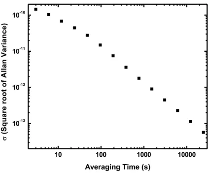
the clock. For the Brazilian atomic beam clock, the short-term stability was determined using a commercial atomic standard (Agilent – 5071A) and a computer with a GPIB interface to store the data reading, allowing us to perform a constant evaluation of the atomic beam standard. Figure 8 shows the measured values of
σ of our Cs133beam frequency standard versus the sampling time τ. For the present evaluation, the short
term stability of the Cs clock isσ (τ )=(6.6±0.2)×10−10τ−0.50+0.1.
FREQUENCYSHIFTS ANDUNCERTAINTIES
Fig. 8 – Square root of the Allan deviation versus the sampling time.
Determination of the Rabi frequency
From the Ramsey fringes one can obtain important operation parameters. The transition rate for the Ramsey interrogation depends on the Rabi frequency. The Rabi frequency is written as,b=(µB/)B, where Bis the microwave magnetic field amplitude in the interrogation region and can be determined by measuring the power of the microwave signal injected into the cavity. The method that we have used makes it easier to ascertain the Rabi frequency by a mathematical analysis of the experimental Ramsey pattern. This analysis provides greater accuracy of the Ramsey pattern (Makdissi and de Clerq 1997). In order to obtain better precision in the determination of the Rabi frequency, we take the second derivative of Eq. (5) and rewrite it as a sum of three Dirac pulses at different frequencies (Teles et al. 2002). The measured value of
b=49,197±16.21 rad s−1is consistent with the operational parameters.
Gravitational and second-order Doppler frequency shifts
These shifts are due to the intrinsic nature of time and space. The most important is the gravitational red shift and the second order Doppler shift.
The Gravitational frequency shift is a relativistic correction due to the gravitational potential variation at a given location on the earth. It is independent of the atomic velocity and just produces a translation shift in the Ramsey fringe.
Clocks on the earth or near to the earth surface, by convention (CCDS 1980) origin of gravitational potential is the geoid surface. This follows the gravitational frequency shift as under (Vanier and Audoin 1989):
νG
ν0
= g
c2H
gravity andcis the velocity of light. Hence the frequency of a clock is an increasing function of its latitude.
The fractional frequency change is 1.09×10⁻¹³ Km−1. The most precise gravitational measurement has
carried been out with a ballistic flight of hydrogen maser. The gravitational effect is red-shifted when the altitude decreases and blue-shifted when altitude increases. The São Carlos altitude, where the atomic beam standard is located, ish=850±50 m. This was measured with a GPS receiver (9390–6000 Datum). The
following is the frequency shift due to the gravitational effect (Teles et al. 2003, Bebeachibuli et al. 2005):
νG
ν0
= −1.0×10⁻¹⁷
The second-order Doppler shift is one of the major frequency shifts in the atomic beam clock. The Doppler effect is always present whenever there is relative motion between the source, observer and prop-agating waves. The atom acts as an observer, emitter and detector. The Doppler effect is always present in gaseous atoms due to their motion unless some special techniques are adopted for its reduction or elimina-tion.
The relativistic approach in case of emission or absorption of electromagnetic radiation makes the 2nd order Doppler effect evident. Therefore higher order terms of the Doppler effect have to considered.
ω=ω0+kυk+ω0 υk2 2c2 −
K2 2M
Hereω0 is the atomic resonance frequency, K is the propagation vector whose magnitude is defined as K = 2λπ = ωc,υkis the velocity of the atoms,cis the velocity of light,is Planck’s constant divided by 2π andM is the mass of atom. The second and third terms are identified with the 1st order and the 2nd order
Doppler effect. The last term represents the recoil effect and it is a function of frequency. Its detection may be possible at high frequencies.
Since the microwave field and the laser fields for optical pumping and detection are all applied orthogo-nal to the atomic beam velocity, the 1st order term can be made negligible. The second-order Doppler effect, however, needs to be considered. The fractional change in the frequency of clock value is expressed as:
ω0
ω0 =
ν0
ν0 = −
υ2
2c2
The second-order Doppler shift is related to the time dilation predicted by the theory of relativity. For each velocity component the shift is given by,
ω= −ω0υ
2
2c2
interpreted as an admixture of P and higher states in the ground state S. However only the quadratic Stark effect produces the shift in the hyperfine structure and this must be considered for clock evaluation. The differential Stark shift induced by the electric field E on the Cesium clock transition is given by (Simon et al. 1998).
ν = −1
2 16
α10
7h − α12
7h
E2
Hereα10 andα12 are the contribution to the cesium static polarizability from contact and the spin-dipolar
interactions respectively, E is the electric field strength andh is Planck’s constant. The value of α12/h
is 10−7smaller than (α
10/h), therefore the second term can be neglected. The value of 8/7×α10/h =
2.273×10⁻¹⁰Hz/(V/m). The measured value of the fractional hyperfine frequency shift for cesium atoms
due to applied electric field is given by
νE
ν0 = −2
.5×10−20E2
where E is the electric field expressed in V/m. This is clearly a very negligible frequency shift. In the
atomic frequency standard there exist no sizable electric field that can be detectable. Therefore we have neglected this effect for Cs beam clock evaluation.
DC magnetic field effect on hyperfine states: Zeeman effect
Atomic Cs primary frequency standards are based on the transition between two levels F = 4, mF = 0 ↔ F = 3, mF = 0. In the absence of a magnetic field all themF sublevels of a given F level are degenerate. So a magnetic field is essential to lift the degeneracy of themF manifold. The value of the required magnetic field (C-field) is very small,≃13µT. The Zeeman effect is expressed according to the
Breit-Rabi equation (Vanier and Audoin 1989)
νm F =νh f s
1+mFx
2 +x
2
wherex = (gJ −gI)/2πνh f s, gI andgJ are the Landé g factors for angular momentum I and J, µB
applicable. The Cs clock operates between themF =0 levels as mentioned above, so the 2nd order shift will effect the accuracy of the clock, and it must be measured with the greatest care (Vanier and Audoin 1989):
νZ
ν0 =4
.2745×1010B02 (7)
Besides the evaluation of transition between mF = 0 other six transitions between mF = ±1, ±2 and
±3 are equally important for determination of clock accuracy. These transitions strongly depend on the
magnetic field. We have observed a shift of 7.3 KHz from the spectrum shown in Figure 4. This value corresponds to the magnetic fieldB0 =13µT. A periodic measurement ofν+1andν−1 are necessary to
observe temporal dependence of the quadratic Zeeman shift. We have measured them for ten days, five time in a day in normal operating conditions and observed that the daily variation is about 5 mHz. Thus relative uncertainty in the temporal measurement of the 2nd order Zeeman shift is
νZ
ν0 =5
.43×10−13 (8)
For details see (Bebeachibuli et al. 2003, 2005, Teles et al. 2002, Santos et al. 2003).
Black body radiation shift
This shift is due to nonresonant excitation of atoms by electromagnetic radiation in thermal equilibrium with the black body at room temperature. The Planck distribution law governs black body radiation. The average electric field and magnetic field energies are proportional to the fourth power of thermodynamic temperatureT4and are given by the following equations (Vanier and Audoin 1989).
E2
=
−1.69×10⁻¹⁴ T 300 4 B2 =
−1.30×10⁻¹⁷
T
300 4
These electric and magnetic fields perturb the cesium atoms by an ac Stark effect and an ac Zeeman effect respectively. Perturbation due to the magnetic field can be neglected because it three orders of magnitude less than the electric field. The operational temperature of the clock isT =296±2 K, resulting in a black
body radiation shift of
νT
ν0 = −(1
.511±0.04)×10−14.
End-to-end cavity phase shift
This shift is related only to the Ramsey type of configuration, and it occurs when there exists a microwave phase difference in the two regions due to losses in the waveguide. In case of a microwave phase difference between the first and second interaction zones, the peak of the Ramsey signal will be shifted. This shift can be expressed as,
ν= ϕ
T = ϕυ
−6.8×10⁻¹²(Teles et al. 2002).
Inhomogeneity of the magnetic field along the microwave cavity
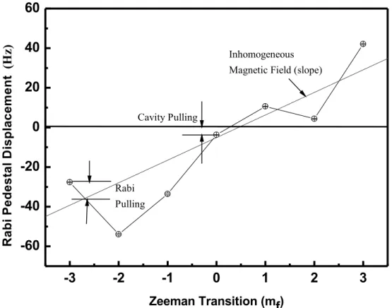
As already discussed, the characteristic signature of an atomic clock is the Ramsey fringe superimposed on a broader resonance called the Rabi pedestal. In ideal conditions, the Ramsey fringe is exactly centered to the Rabi pedestal. However, if there is any magnetic field inhomogeneity along the atom trajectory through the microwave cavity the Ramsey fringe is no longer centered on the Rabi pedestal and a frequency shift is induced.
For the measurement of the inhomogeneity of the magnetic field we undertook to measure the position of the Ramsey fringe with the Rabi pedestal for themF =0 transitions. The difference between them was computed and written as (Makdissi and de Clerq 2001)
D(mF)=νRam(mF)−νRabi(mF)=ν0 mF
8
(ǫ1+ǫ2)
whereǫ1andǫ2are fluctuations of the mean static field in the first and second interaction regions
respec-tively. The slope in the linear curve of D(mF) as a function of mF determines the value of (ǫ1+ǫ2).
As seen in Figure 9, the slope in the experimental curve D(mF) ×mF is 11.35 ±0.05 resulting in
(ǫ1 +ǫ2) = −0.99 ±0.05 ×10⁻⁸. This yields a frequency error on the clock transition due to the
field inhomogeneity ofνz = 1.08±0.04×10⁻⁵ Hz. The other Zeeman transitions are also shifted by the same effect, and they are shifted by 0.77µHz. The detailed analysis procedure is given in articles
(Bebeachibuli 2003, 2005, Santos et al. 2003). The results are computed in terms of total uncertainty considering the uncertainty measured due the experimental determination of the Zeeman frequency,
νZ
ν0 =5
.43×10−13
and the correction due to the field inhomogeneity,
νZ
ν0
=0.08×10⁻¹³.
The quadratic sum of these terms results in
νZ
ν0
=5.5×10⁻¹³
Rabi Pulling
Besides the chosen clock transition, there are the other six Zeeman transitions whose energies depend linearly on the static magnetic field (C-field),F = ±1;mF =0, as shown in Figure 4. The separation between the neighboring transition and the clock transition is 92 KHz which corresponds to a 13µT C-field.
These transitions have finite line width and hence they overlap the clock transition. Rabi Pulling is due
to the superposition of the pedestals between adjacent transitions in the Zeeman spectrum. The transition signal of the first neighbor(mF =0)is written as,
s(0)=I(0)P(0)+I(1)P3(0−ωz)+I(−1)P3(0+ωz) (9)
whereP(0)is the Ramsey probability and P3(0)is the Rabi pedestal,I(m)is the amplitude of transition mandωz =2π νz. The probabilityP3(0)is given by the equation
P3(0)= b 2
20[1−cos0τ]≃ b2 20.
Expanding this equation in first order in 0
ωz
, we obtain
P3(0−ωz) =
b2 ω2z
1+20 ωz
(10)
P3(0+ωz) =
b2 ω2z
1−20
ωz
If we insert Eqs. 10 into Eq. 9 and rewriting terms we obtain
s(0)= P(0)+β0+0β1 (11)
where
β0 =
b2I(1)+I(−1)
I(0)ωz2
(12)
β1 =
2b2
I(1)−I(−1)
I(0)ω3z
From Eqs. 11 and 12 we see that the effect of the neighbors’ transition on the clock transition is expressed by a small even quantityβ0and an odd functionβ1. The odd function creates a deformation of the clock
signal. When the neighbor transitions,mF = I andmF = −I, have the same amplitude the deformation vanishes. The frequency shift induced may be calculated by,
νRabi = −
β1ωm
π A(ωm,b, τ ) f(τ )dτ
Cavity pulling arises from the variation of the microwave amplitude with frequency when the cavity is mistuned. It is nearly independent ofmF, but it has a strong dependence on the microwave power and on the modulation amplitude. Our procedure to measure the cavity pulling is the same as was used to measure the magnetic field inhomogeneity. From Figure 9 the measured pedestal shift is 3.76±0.10 Hz
and the induced effect on the Ramsey fringe for the cavity detuning is 1.27×10⁻¹³for the clock transition
(Bebeachibuli et al. 2003, 2005).
Fig. 9 – Frequency difference between the center of the Ramsey fringe and the Rabi pedestal as a function of the Zeeman sublevels
GLOBALACCURACYBUDGET
The accuracy of an atomic frequency standard is defined as the capacity of the standard to produce a frequency that is in agreement with the definition of the second. It is expressed as a relative uncertainty ν
υ0
, relative to the second definition. Applying the several corrections to our frequency standard, their corresponding uncertainties are tabulated in Table I.
TABLE I
Global accuracy budget.
Frequency Shift Correction(1×10⁻¹³) Uncertainty(1×10⁻¹³)
Red Shift −1×10⁻⁴ −5×10⁻⁵ 2nd order Doppler −1.65 0.12
Quadratic Zeeman 5.5 0.15
Cavity Pulling 1.27 0.09
Rabi Pulling 1.3 0.05
Black Body Radiation −0.2887 0.004
Finally, the global accuracy of the beam standard results inσC=6.13×10⁻¹³. This value means that the precision at which our frequency standard measures the clock transition frequency is 9 192 631 770 Hz. This uncertainty is comparable with the available commercial beam clocks. The constructed device was an important step on the learning curve for the Brazilian team towards the fountain clock development that will be described in the next section.
CONSTRUCTION AND EVALUATION OF THE CESIUM FOUNTAIN CLOCK
Time and frequency metrology is a dynamic field. As the technology advances, new and more precise ways to measure time arise. The fountain clock is an important step with about three orders of magnitude improvement over the current atomic beam clock. In order to master the state-of-the-art in the field of time and frequency standards, we decided to undertake development of anatomic fountain clock.
Why is a fountain clock better than the conventional atomic beam?
The Ramsey two-interaction-zones technique demonstrates that the full-width-half-maximum(FWHM) of the central fringe is proportional to (1/T) or (υ/L). This imposes two limits in the achievement of
narrower Ramsey fringe and hence improvements over the accuracy of thermal beam clock: the cavity lengthLincrement and the atomic velocity (υ) reduction. The thermal atomic beam cannot be made slower
than 70 ms−1due to the intrabeam collisions and velocity distribution. The length of cavity is limited by
the beam shape and loss of the atoms. Thus the shape of velocity distribution and correct geometry put an upper limit on the thermal atomic beam clock. A typical tube with a 1 m drift region and velocity of 100 ms−1results in a 10 ms interaction time or 50 Hz line width.
to the thermal beam clock. Besides the most advantageous aspect of line width reduction, another benefit of the fountain clock configuration is the trajectory reversal that removes the cavity end-to-end phase shift and eliminates the distributed cavity phase effects. The first fountain clock was developed at the Observatoire de Paris, France and exhibited a relative uncertainty of 1.1×10⁻¹⁵ (Clairon et al. 1996, Wynands and
Weyers 2005).
CONSTRUCTION
Device description
The construction of a cesium cold atom fountain frequency standard is described in detail in (Magalhães et al. 2003) and shown in Figure 10.
It consists of ultrahigh vacuum pumps, a magneto-optical trap (MOT), stabilized diode lasers, a micro-wave synthesizer, free-flight cylinder and detection regions. The vacuum system consists of two parts, one for the trapping chamber and another for the free-flight cylinder. The background pressure in the chamber, lower than 10−7Pa, was maintained by a 60 ls−1ion pump. The MOT vacuum chamber is made
of stainless steel having dimensions 35 cm in length and 20 cm in diameter. The MOT operates with the trapping beams meeting at the center orthogonally and tuned to the D2 line of cesium. In this geometry
3 upper and lower trapping beams make an angle of 35.4◦with respect to the horizontalx-y plane.
Anti-Helmholtz coils are mounted along the y-direction for the generation of magnetic field. The detection region is about 19 cm below the trapping region as shown in Figure 10. The free-flight cylinder is 90 cm in height and 1.5 cm in diameter. It is made of copper (nonmagnetic) to reduce the effects of residual magnetic fields inherent in stainless steel.
The microwave cavities for the interrogation and preparation regions are made inside the free flight chamber. These cavities couple the TE011mode of the microwave signal. They are resonant at the clock rf
Fig. 10 – The scheme of the atomic fountain. The C-field region is about 79 cm high. The microwave cavity is 29 cm above the magneto optical trap and the detection zone 17 cm below the trap. The atomic populations, NF=3and NF=4, are measured
atomic fluorescence.
The cycling process of the atomic fountain is stated with the preparation of cold atoms in the MOT. Then to produce a homogeneous atomic cloud, the magnetic field is turned off and atoms are exposed to a molasses phase. Then the cold atoms cloud is launched using the moving molasses technique. The initial velocity of launched atoms is determined by the frequency detuning between upper and lower laser beams at 852 nm. During this phase the trapped atoms are detuned adiabatically far from the resonance that results in a sub-Doppler cooling of the cloud.
The principal laser source for trapping and cooling the atoms is a diode laser system model TA 100 from TOPTICA. The laser is locked to the reference Cs cell using the conventional saturated absorption technique. In the reference system an acousto-optic modulator (AOM) shifts the laser frequency and provides the detuning control for the MOT and sub-Doppler cooling phase. The optical output from the TA 100 is divided by using polarizing cubes, and each beam passes through separate AOMs. The voltage controlled oscillator (VCO) that supplies RF signal to these two AOMs insures that they are phased-locked for the MOT and optical molasses production. For launching the atoms, a frequency difference is introduced between the upper and lower beams by an external digitally derived synthesizer (DDS) through the two AOMs. A repumper consisting of an external cavity diode laser system is used to pump the atoms from 62S
1/2F =3→62P3/2F =4. A part of the laser beam is split and propagated through another reference
Cs cell while the rest of the repumper maintains stability and correct functioning of the MOT. A third diode laser (SDL5412-H1) is used for the detection of atoms. It is locked to the 62S
1/2F =4 →62P3/2F =5
beam is about 11 mW and diameter is about 28 mm. Using this cycling process, and launching the cold atoms 10.5 cm above the microwave cavity, we obtained a 1.7 Hz wide Ramsey central fringe. With this signal, the short-term stability was 6.6×10⁻¹².
Microwave synthesizer
To produce the interrogation signal to the atomic fountain experiment, a microwave synthesizer was constructed with the valuable collaboration of the LNE-SYRTE (Laboratoire National de Métrologie et d’Essais–Systèmes de Référence Temps-Espaces) time-and-frequency team. This chain, shown in Fig-ure 11 uses a similar topology to some devices already operating with their atomic frequency standards [4]. It has the same core idea used in the NIST chain, that is to generate a signal with the best spectral charac-teristics of high performance oscillators using phase-locked-loop techniques.
The main parts of the synthesizer are the three oscillators: 4.596 GHz (DRO – Dielectric Resonant Oscillator – 4R596-10SF – Omega Technologies), 10 MHz (BVA – OCXO 8600 – Oven Controlled Crystal Oscillator – Oscilloquartz) and 100 MHz (500-07542A – Wenzel Associates Inc). The 100 MHz crystal oscillator is phase locked to the BVA at low frequencies (below 30 Hz), providing an output signal at 100 MHz with phase noise characteristics superior to each component individually. This 100 MHz signal is then doubled and inserted into a sampling mixer (RF – Reference Frequency input), which performs the subtraction of the 23rd harmonic of this input (4.6 GHz) with the main harmonic signal coming from the DRO at 4.596 GHz (LO – Local Oscillator input). The output signal from the sampling mixer (IF – Intermediate Frequency) is compared with an external 29.5 MHz frequency, supplied by a DDS (SR345 – Stanford Research Systems) that uses the BVA as an external reference. This comparison provides the phase locking of the DRO, allowing modulation through the DDS programming. The other DRO output is connected to a waveguide filter whose band is centered on its first harmonic at 9.192 GHz. The signal output has−15 dBm of output power, that is more than enough to feed the resonant cavity with a quality
factor better than 5000 and minimizes spurious fields from connection leakages. The direct modulation of the DRO also provides an excellent way to increase the step resolution of the chain. Since the frequency step in the SR-345 is microhertz, the division by 8 provides a double advantage. The first advantage is that the frequency step resolution is 2.5×10⁻⁷Hz. The second is provided by the fact that the signal synthesis
is digitally performed, so the phase noise is not increasing with frequency. Using this fact, and since the DDS maximal frequency is 30 MHz, the 29.5 MHz signal is set, and a frequency division by eight also divides the signal phase noise by the same amount, improving the quality of the signal. This synthesizer was compared to other similar chains, and the obtained stability was shown to be 9.7×10⁻¹⁴τ−1/2. To supply
the microwave preparation signal, part of the 200 MHz signal generated in the first synthesizer is used to drive a second high-frequency phase lock, in the same topology used as in the first chain. In this case, a DRO at 9.192 GHz (10.84 dBm) is inserted into a sampling mixer and subtracted from the 46th harmonic of a 200 MHz signal derived from the interrogation chain. The sampling mixer output is compared with a 7.3 MHz signal provided by a DDS (SR345 – Stanford) and phase locks the DRO. In order to avoid perturbing fields during the interrogation phase, after the atoms pass the preparation cavity, the signal is switched off by the temporal sequence controller. This is done by using a switch with 80dB of isolation (F192A – General Microwave).
CONSTRUCTION AND EVALUATION OF THE EXPANDING COLD ATOM CLOCK
magneto-optical trap (MOT). A microwave antenna is used to provide the microwave radiation for the clock transition, which is detected by the fluorescence from the optically pumped excited states.
Fig. 12 – Schematic diagram of experimental setup for expanding cold atomic clock.
Figure 12 illustrates the simplified schematic diagram. A cesium vapor cell can be pumped to a base pressure≃ 10−7Pa. A temperature-controlled reservoir allows regulating the amount of Cs atoms
into the glass cell. Around the glass cell two main coils produce the magnetic field for magneto-optical trapping of the atoms and a set of compensation coils guarantee a field-free environment for the atomic cloud expansion. Atomic densities≃ 1010 cm−3are typically measured by fluorescence. Two stabilized
diode lasers provide the frequencies necessary to produce the cooling and repumping light. The relevant transitions excited by the lasers are the 62S
1/2F =4 → 62P3/2F =5 cycling transition and the 62S1/2F =
3 → 62P3/2F =4 repumping transition, that prevents atoms from accumulating in theF =3 ground state
during the trapping phase of the experiment. The trapping and repumping beams are spatially overlapped and divided along three orthogonal axes. Two counterpropagating beams intersect in the horizontalx−y
plane and the third beam is directed along thezaxis, perpendicular to thex−yplane and passing through
located 10 cm from the cell center. A microwave antenna of quarterwave is positioned perpendicular to the vertical axis, outside the glass cell and about 3 cm from the atoms. The radiation pattern of the antenna was determined so as to position the atoms in the high-intensity region. The antenna was coupled to a microwave chain, generating 9.192 GHz. About 2×10⁸atoms are captured in the MOT and become the
sample for performing the microwave transition and to lock the oscillator chain. The time sequence used to observe the microwave resonance is the following: for about 800 ms, the magnetic field of the MOT, as well as the lasers, are turned on, allowing capture and accumulation of atoms. The repumping laser and the MOT coils are then turned off until the end of the sequence. For the next 23.9 ms the trapping laser is still on and will promote optical pumping of the atoms to the 62S
1/2F =3 state, after which it is
turned off. At this stage the atomic cloud is in free expansion and remains so for the next few ms. Then the first microwave pulse of duration 2 ms is applied. After a quiescent interval of 8 ms, a second pulse of microwave can be applied or not. At the end, the trapping laser is turned back on for 50 ms and the fluorescence of atoms at 62S
1/2F = 4 is detected. The atoms originally populated in 62S1/2F = 3 are
transferred to 62S
1/2F = 4 by the microwave field. A variable attenuator is placed on the microwave
source such that aπ-pulse is applied during thetpperiod (Rabi method). In the case of two consecutive pulsestp, the microwave power is adjusted to produce twoπ/2-pulses (Ramsey method). The temporal sequence for the experiment is illustrated in Figure 13. The fluorescence detection system is composed of a collecting lens that images the cloud onto a calibrated photodetector. Once the resonance line is obtained, a modulation of the microwave frequency allows generates the error signal used to lock the oscillator on the atomic resonance. The microwave chain is phase-locked (phase-locked-loop) to the 10 MHz output of a commercial standard oscillator source (Magalhães et al. 2006, Müller et al. 2005).
Fig. 13 – Timing sequence of applied pulses used to control the expanding cold-atom clock experiment.
EVALUATION
was obtained with a Cs beam and a 4 m long transition region (Glaze et al. 1977), we can appreciate the great potential for the use of the cold-atom Rabi interrogation method as a clock transition. In terms of line width vs. length of transition region, we are three orders of magnitude better than conventional beam clocks. Compared to atomic fountains, whose typical line width is 1 Hz, we see that there is also room for improvement when just a cloud of cold atoms is used.
Fig. 14 – Resonance observed in the expanding cold-atom experiment using 12 ms ofinterrogation time in a Rabi method. The resonance observed in Figure 14 was used as a clock transition to lock a local oscillator. The generated error signal was used to evaluate the comparison thus obtaining the Allan variance. The frequency stability of the produced clock is presented in Figure 15, resulting in an Allan standard deviation ofσ (τ )= (9± 1)×10−11τ−1/2, already a good stability considering the simplicity of the device. There is still a lot
of room for improvement, and we should be able to obtain a result about one order of magnitude better for short-term stability. It should be straightforward to extend the present demonstration technology to make a compact high performance, all-optical atomic clock, with a long lifetime of Cs supply compared to present Cs tube lifetimes.
Fig. 15 – Frequency stability plot for the expanding cold-atom clock against a commercial Agilent 5071A reference.
attempt to implement the Ramsey method. In this case we have usedtp =2 ms andtb = 8 ms, with a power level such that aπ/2-pulse condition for each interrogation is satisfied. The existence of fringe is
quite clear but with very poor contrast. The reason for this poor contrast are not yet entirely understood. It seems that the fringes exhibit a great narrowing of the transition but the poor contrast makes it hard to lock an oscillator as has been done for the single-interaction-zone, Rabi profile. The possible reasons for this poor contrast are under investigation.
CONCLUSION
In this article we have discussed the important applications of atomic clocks, their working principles, based on the two separated microwave interaction zones, and the different types of cesium atomic clocks. We have thoroughly described the cesium-based Brazilian program, construction and evaluation.
We have designed and developed the cesium beam clock, fountain clock and compact cold atom clock under the research program on time and frequency metrology in Brazil. These are the first thermal and cold atoms standards fully constructed in Latin America.
The construction of the Brazilian frequency standards family has been described in detail. It consists of cesium oven, beam chamber, vacuum systems, microwave cavity, C-field, graphite discs, diode laser, diode laser driver and stabilizer, microwave synthesizer, magneto-optical trap (MOT) and free flight cylinder.
Evaluation of the frequency standards was performed and based on experimental data. Short term stability of the clocks was determined from the square root of the Allan variance. The short term stability of the beam clock, fountain clock and compact expanding cold atom clock were determined to beσ (τ )= (6.6±0.2)×10−10τ0.5±0.1, σ (τ )=(6.6±0.2)×10−12τ0.5, and σ (τ )=(9±1)×10−11τ0.5respectively.
ACKNOWLEDGMENTS
The authors acknowledge the financial support obtained from Fundação de Amparo à Pesquisa do Es-tado de São Paulo, Centros de Pesquisa, Inovação e Difusão, Centro de Pesquisa em Óptica e Fotônica (FAPESP/CEPID/CePOF), Coordenação de Aperfeiçoamento de Pessoal de Nível Superior (CAPES/ COFECUP) and Conselho Nacional de Desenvolvimento Científico e Tecnológico (TIB-CNPq). We also acknowledge the important collaboration with LNE-SYRTE. M.A. also acknowledges support from the higher education commission of Pakistan.
RESUMO
Relógios atômicos de feixe de Césio têm sido a base para diversas aplicações em ciência e tecnologia nas últimas quatro décadas. Testes de leis fundamentais de física, buscas por mínimas variações em constantes fundamentais, sincronização de redes de telecomunicações e o funcionamento do sistema de posicionamento global, baseado em satélites de navegação, não seriam possíveis sem os relógios atômicos. A adoção de técnicas de aprisionamento e resfriamento ópticos tem permitido um grande avanço na precisão dos relógios atômicos. Chafarizes de átomos frios e relógios compactos de átomos frios também têm sido desenvolvidos. Precisões de medida de algumas partes em 1015 foram demonstradas para relógios do tipo chafariz de átomos frios. Apresentamos uma visão geral do programa de metrologia de tempo e freqüência baseado em átomos de césio, em desenvolvimento na USP de São Carlos. Estas atividades consistem na construção e caracterização de relógios do tipo feixe atômico e de outros, utilizando átomos frios. Discutimos os princípios básicos, construção, avaliação e importantes aplicações de relógios atômicos no programa brasileiro.
Palavras-chave:Relógio atômico, átomos frios, tempo e freqüência, metrologia.
REFERENCES
ALLANDW. 1966. Statistics of atomic frequency standards. Proceedings of IEEE 54: 221–230.
ALLANDW. 1989. In seach of the bet clock: An update in: Frequency standards and metrology. Springer, Berlin, Heidelberg.
ALLANDW, KUSTERS JANDGRIFFREDR. 1994. Civil GPS timing application. Proceedings of ION GPS-04,
AUDOINCANDGUINOTB. 2001. The Measurement of Time: Time, Frequency and The Atomic Clock. Cambridge
University Press.
BAUCHA. 2003. Cesium atomic clock: function, performance and applications. Meas Ci Technol 14: 1159–1173.
BEBEACHIBULIA, SANTOS MS, MAGALHÃESDV, TELESFANDBAGNATOVS. 2003. Characterization of the frequency pulling by magnetic field oscillation of the Brazilian Cs atomic frequency standard. Proceedings of the 2003 IEEE International frequency control symposium, p. 95–99.
BEBEACHIBULIA, SANTOSMS, MAGALHÃESDV, MÜLLERSTANDBAGNATOVS. 2005. Characterization of
the main frequency shifts for the Brazilian Cs atomic beam frequency standard. Braz J Phys 35: 1010–1015.
BIZESET AL. 2005. Cold atom clocks and applications. J Phys B 38: S449–S468.
CASENAVEA, BONNEFONDP, DOMINHKANDSCHAEFFERP. 1997. Caspian Sea-Level from TOPEX/
POSEI-DON Altimetry Level Now Falling. Geophys Res Lett 24: 881–884.
CCDS. 1980. Proceedings of the Consultive Committee for the Definition of Second Bureau International des Poids et Mesures, Sèvres, France.
CGPM. 1967. 13th General Conference on Weights and Measures.
CLAIRONA, SALOMONC, GUELLATI SANDPHILLIPSWD. 1991. Ramsay Resonance in a Zacharias Fountain.
Europhys Lett 16: 165–170.
CLAIRONA, GHEZALIS, SANTARELLIG, LAURENTPH, LEASN, BAHOURAM, SIMONE, WEYERSS AND
SZYMANIEC. 1996. Preliminary accuracy evaluation of a cesium frequency standard. Proceeding of the 5th
Symposium on Frequency Standards and Metrology, p. 49–59.
ESSEN LAND PARRYJVL. 1957. The cesium resonator as a standard of frequency and time. Phil Trans R Soc A250: 510–514.
FEENSTRAL, ANDERSSON LMANDSCHMIEDMAYERJ. 2004. Microtraps and atom chips: Toolboxes for cold
atom physics. Gen Rel and Grav 36: 2317–2329.
FLAMBAUMVVANDTEDESCOAF. 2006. Dependence of nuclear magnetic moments on quark masses and limits
on temporal variation of fundamental constants from atomic clock experiments. Phys Ref C 73: 055501.
GLAZEDJ, HELLWIG H, ALLANDWAND JARVISS. 1977. NBS-4 and NBS-6: The NBS Primary Frequency
Standards Metrologia 13: 17–28.
GODONEA, NOVEROC, TEVALLEPANDRAHIMULLAHK. 1993. New experimental limits to the time variations of gp (me/mp) andα. Phys Rev Lett 71: 2364–2366.
GUILLOTE, POTTIEPE, VALENTINC, PRTITPANDDIMARQN. 1999. Proceedings of the 1999 Joint meeting
of the European Frequency and time forum and the IEEE International frequency control symposium, p. 81–84.
HAFELEJCANDKEATINGRE. 1972. Around the worls atomic clocks. Predicted relativistic time gains. Science
177: 166–168.
JESPERSONJANDFITZ-RANDOLPHJ. 1999. From sundials to atomic clocks: understanding time and frequency. Dover publications.