UNIVERSIDADE TÉCNICA DE LISBOA
INSTITUTO SUPERIOR DE ECONOMIA E GESTÃO
MESTRADO EM: ECONOMIA MONETÁRIA E FINANCEIRA
EXCESS RETURNS AND NORMALITY
JOÃO PEDRO DO CARMO BOAVIDA
Orientação: Doutor Paulo Brasil de Brito
Júri:
Presidente: Doutora Maria Rosa Borges
Vogais: Doutor José Dias Curto
Abstract
In this dissertation, I assess under which circumstances normality can be a good descriptive
model for the U.S. excess returns. I explore two possible sources of deviations from
normal-ity: structural breaks and regime switching in long term aggregate time series. In addition,
I study temporal aggregation (i.e., considering the frequency of data as a variable) for
ex-cess returns in short term time series. My main findings are summarized as follows. First,
using long spanning monthly time series data from 1871 to 2010, I find that (1) there are
structural breaks in monthly excess returns between pre-WWII and post-WWII data; and,
(2) while pre-WWII data is consistent with normality, post-WWII data is not. Second, I
provide evidence of two market regimes for excess returns in post-WWII data. These regimes
may be seen as bull and bear market conditions. Third, using high frequency post-WWII
data, I check for aggregational Gaussianity, from daily to annual data. I find that
Gaus-sianity depends on the frequency of data: it may hold for highly aggregate data (starting
from semi-annual to annual data) but it does not hold for high frequency data (less than
semi-annual). My main contribution is to demonstrate the ”normality survival” when
fre-quency is taken as a variable. After a careful look at the available literature on aggregational
Gaussianity, I found no previous applications and results for excess returns.
Keywords: Excess returns, Normality, Structural breaks, regime switching, Time
aggre-gation
Resumo
Nesta disserta¸c˜ao, eu avalio sob que condi¸c˜oes a normalidade pode ser um bom modelo
des-critivo para os excess returns nos E.U.A.. Para tal, exploro duas fontes potenciais de desvio
da normalidade: quebras de estrutura e mistura de regimes para s´eries temporais longas
agregadas. Adicionalmente, estudo a agrega¸c˜ao temporal (i.e., tomando a frequˆencia dos
dados como vari´avel) para os excess returns em s´eries temporais. Os principais resultados
obtidos s˜ao os seguintes. Primeiro, utilizando dados mensais para um longo perodo temporal
de 1871 at´e 2010, conclui-se que: (1) existem quebras de estrutura nos excess returns mensais
entre o per´ıodo antes e depois da Segunda Guerra Mundial (SGM) e, (2) enquanto os dados
do per´ıodo antes da SGM s˜ao consistentes com a normalidade, os dados do p´os-guerra n˜ao
s˜ao. Segundo, apresenta-se evidˆencia de dois regimes de mercado para o per´ıodo p´os-SGM.
Estes regimes podem ser vistos como descrevendo condi¸c˜oes de mercadobull ebear. Terceiro,
usando dados com frequˆencias mais altas para o per´ıodo p´os-SGM, testa-se a aggregational
Gaussianity para dados de di´arios at´e dados anuais. Conclui-se que a Gaussianity depende
da frequˆencia dos dados: pode ser v´alida para dados mais agregados (come¸cando em
da-dos semestrais at´e dada-dos anuais) mas n˜ao ´e v´alida para dada-dos com frequˆencias mais altas
(menores que semestrais). O principal contributo desta disserta¸c˜ao ´e demonstrar a
sobre-vivˆencia da normalidade quando se toma a frequncia dos dados como vari´avel. Ap´os uma
revis˜ao aprofundada da literatura sobreaggregational Gaussianity, n ao encontrei resultados
anteriores para osexcess returns.
Keywords: Excess returns, Normalidade, Quebras de Estrutura, Regime Switching, Agrega¸c˜ao
Temporal
Agradecimentos
Ao Professor Doutor Paulo Brito pela sua preciosa colabora¸c˜ao e pela sua forma ´unica de
levar o conhecimento a um n´ıvel mais alto. Ao Professor Doutor Lu´ıs Costa pelos seus
conselhos que me acompanharam ao longo da minha vida acad´emica no ISEG. `A Joana pela
sua compreens˜ao e o seu carinho demonstrado nos momentos mais dif´ıceis. `A minha irm˜a e
aos meus pais pelas palavras de incentivo em superar este desafio. A Deus pela f´e em tornar
Contents
1 Introduction 1
2 Excess returns and normality 4
2.1 Excess returns - a definition . . . 4
2.2 Normality and Itˆo calculus . . . 4
2.3 Monthly series and some stylized facts . . . 7
2.3.1 Data . . . 7
2.3.2 Moments . . . 8
2.3.3 Normality tests . . . 11
3 Characterizing deviations from normality 13 3.1 Structural breaks . . . 13
3.1.1 Methodology . . . 14
3.1.2 Tests results . . . 17
3.1.3 Normality in different subperiods . . . 22
3.2 Regime Switching . . . 23
3.2.1 Gaussian mixture model . . . 24
3.2.2 Expectation-maximization . . . 25
3.2.3 Number of regimes . . . 27
3.2.4 Parameter estimates . . . 28
4 Time aggregation and Normality 31 4.1 Data . . . 32
4.2 Aggregational Gaussianity . . . 33
4.3 Normality tests . . . 35
List of Figures
1 Time series of U.S. monthly excess returns . . . 8
2 Empirical density of excess returns and the Normal PDF . . . 9
3 Stability tests in the conditional mean of excess returns . . . 18
4 Stability tests in the conditional variance of excess returns . . . 20
5 BIC (and RSS) values for different number of breakpoints. . . 21
6 Empirical density of excess returns and the PDF mixture of two Normal dis-tributions . . . 30
7 Empirical density of excess returns and the Normal PDF for different levels of aggregation . . . 33
List of Tables
1 Descriptive statistics . . . 82 Excess returns: empirical frequencies vis-`a-vis Normal distribution . . . 10
3 Normality tests in excess returns . . . 12
4 Breakdates found in the conditional variance of excess returns . . . 21
5 Descriptive statistics for excess returns over different periods . . . 23
6 BIC values for different numbers of regimes in excess returns . . . 28
7 BIC values for different number of regimes in excess returns over post-WWII data . . . 30
1
Introduction
Normality of excess returns is maybe the central assumption in finance and macrofinance.
Normality allows for the use of a powerful instrument such as the Itˆo calculus, which is
the stepping stone of most of the results in theoretical asset pricing. However, empirical
results have systematically pointed out to deviations from normality. In almost all the cases
it has been established that empirical distributions of returns are skewed and leptokurtic
(Mandelbrot, 1963; Fama, 1965; Campbell et al., 1997).
Should we consider most of finance theory as unrealistic, and therefore irrelevant? Should
we just use empirical measurement without theory given the lack of appropriate theoretical
background?
In this dissertation, I try to assess under which circumstances normality can be a good
descriptive model for the U.S. excess returns. There are several reasons why normality may
not hold. One branch of the literature studies deviations from normality assuming that
parameters are time-varying, that is, assuming non-stationarity. In this context, deviations
from normality in financial returns may arise if these are mean-reverting (Poterba and
Sum-mers, 1988) or characterized by GARCH features (Bollerslev et al., 1992). I explore other
possible sources of deviations from normality: structural breaks and regime switching in long
term aggregate time series. The existence of structural breaks or regime switching may
pro-vide a solution to obtain normality for excess returns conditional on subperiods or regimes,
respectively. In addition, I study temporal aggregation (i.e., considering the frequency of
data as a variable) for excess returns in short term time series.
The standard approach to test normality for excess returns uses the sample estimate of
the mean and the sample estimate of the variance for a given sample period. This approach is
acceptable if excess returns are assumed to be independent and identically distributed (i.i.d.)
and, therefore, the estimated parameters - mean and variance - remain constant for the entire
sample period. However, when long histories are being used, stationarity may not hold: for
be changing over time, experiencing shifts known as ”structural breaks”, or switching among
a finite set of values, that is, they are ”regime-switching”.
Deviations from normality, such as structural breaks or regime switching, have been found
for excess returns. P´astor and Stambaugh (2001) estimated the expected U.S. excess return
in a Bayesian framework in which the prior distribution is subject to structural breaks. They
reported a total of fifteen structural breaks for excess returns using a sample period covering
1834-1999. The most significant break, however, was found to be in the late 1990s.
Kim et al. (2005) adopted also a Bayesian likelihood analysis to compare four univariate
models of excess returns using monthly data for a shorter sample period covering 1926-1999.
They constructed Bayes factors based on the marginal likelihoods, which allowed them to
make model comparisons and to test structural breaks. Their findings are similar to mine.
First, they found statistical evidence of a structural break in excess returns around the
WWII period. In particular, they found that there is a permanent reduction in the general
level of stock market volatility in the 1940s. My methodology finds support of breaks in the
variance but not in the mean of excess returns. Second, Kim et al. (2005) found that the
empirical Bayes factors strongly favour the three models that incorporate Markov switching
volatility over the simple iid model. My findings support evidence of two market regimes
possibly connected with two different business cycle stages. In particular, I observe times
where excess returns are expected to be low and highly volatile and times where, in contrast,
excess returns behave in the opposite way.
Empirical research also indicates that the shape of the distribution of stock returns is not
the same for different time scales (Cont, 2001 and Eberlein and Keller, 1995). For instance,
it has been established that daily returns depart more from normality than monthly returns
do (see, e.g., Blattberg and Gonedes, 1974; Eberlein and Keller, 1995; and Campbell et
al., 1997). Campbell et al. (1997) compared the distributions of daily and monthly stock
returns for two indices and ten stocks from the U.S. for the period 1962–94. They found
of monthly data is significantly lower than that displayed by the distributions of daily data.
This stylized fact, also known as ”aggregational Gaussianity”, indicates that as one increases
the time scale over which returns are calculated their distribution looks more and more like
a normal distribution (Cont, 2001). In particular, it has been observed that, as we move
from higher to lower frequencies, the degree of leptokurtosis diminishes and the empirical
distributions tend to approximate normality.
My main findings can be summarized as follows. First, using long spanning monthly time
series data from 1871 to 2010, I find that (1) there are structural breaks in monthly excess
returns between pre-WWII and post-WWII data; and, (2) while pre-WWII data is consistent
with normality, post-WWII data is not. Second, I provide evidence of two different market
regimes for excess returns in post-WWII data. These regimes may be seen as bull and bear
market regimes. Third, using high frequency post-WWII data, I check for aggregational
Gaussianity, from daily to annual data. I find that Gaussianity depends on the frequency of
data: it may hold for highly aggregate data (starting from semi-annual to annual data) but
it does not hold for high frequency data (less than semi annual).
In this dissertation, I incorporate two branches of literature that study deviations from
normality in excess returns: (i) one that tests for the existence of structural breaks and
regime switching and (ii) other that explores time aggregation. After a careful look at the
available literature on aggregational Gaussianity, I found no previous applications and results
on excess returns. My main contribution is to demonstrate the ”normality survival” when
frequency is taken as a variable.
This dissertation is organized as follows. In section 2, I define excess returns and I
present the formal proof for the normality of log excess returns as well as some stylized
facts for monthly excess returns. In Section 3, I test if non-normality is associated with the
presence of structural breaks and regime switching for monthly data. In Section 4, I test for
2
Excess returns and normality
2.1
Excess returns - a definition
Total returns for stocks are defined as the sum of returns from capital gains and reinvested
dividends from a market stock index. Let Pt be the average price value of the stock index
at period t and Dt the average dividend payment between periods t−1 and t. Thus, the
continuously compounded return on the aggregate stock market at time t is
rt =log(Pt+Dt)−log(Pt−1).
In addition, letrtf denote the average log-return on a riskless security at periodt.
Typi-cally, yields from long-term Government Bonds have been used as a proxy for the relatively
risk-free asset.
Excess return can be seen as the risk premium paid to investors for holding stocks - which
are risky - instead of riskless securities. In this sense, the excess return may also be thought
of as the payoff on an arbitrage market portfolio where investors go long on stocks and take
short positions on riskless securities. In such market portfolio, the continuously compounded
excess return at time t is defined by
zt =rt −rft.
2.2
Normality and Itˆ
o calculus
Normality allows for the use of the Itˆo calculus, which is the stepping stone of almost all
the results in theoretical asset pricing. In continuous-time asset pricing models, financial
prices are assumed to be geometric Brownian motions, and, therefore, by the Itˆo’s lemma,
logarithmic returns follow a Normal distribution. This lognormality assumption is used, for
In this part, using a continuous-time framework, I present the formal proof that the log
excess returns are normally distributed.
Let the time be continuous and consider two assets: X1(t) being the stock price and
X2(t) the risk-free price1. For the sake of simplicity, I assume for these assets that there
are no accruing dividends nor accruing interest. The stochastic processes for the risky asset
X1(t) and for the riskless assetX2(t) follow two diffusion processes,
dX1(t) =µ1X1(t)dt+σ1X1(t)dW(t)
and,
dX2(t) =µ2X2(t)dt+σ2X2(t)dW(t)
where µ1 and µ2 represent the expected rate of return and σ1 andσ2 the expected volatility.
I explicitly assume that these parameters are constant and, therefore, that the processes are
stationary. In addition, I consider that these two asset prices are subject to the same source
of uncertainty, dW, which follows a standard Wiener process2.
Let the excess returnsZ(t) be defined by Z = X1
X2, or in logarithms by,
z = ln
X1
X2
= ln (X1)−ln (X2)
Itˆo’s lemma, which is a stochastic calculus theorem, yields an equivalent continuous-time
equation for the dlnX1(t) and dlnX2(t). To illustrate this, let F(X1(t), t) = ln (X1(t))
and G(X2(t), t) = ln (X2(t)) be functions of the log prices of the underlying assets X1 and
X2 and timet. Therefore, from the Itˆo’s lemma,dlnX1(t) anddlnX2(t) are also stochastic
1
Without loss of generality, assume a small value of volatility for the riskless asset.
2
process, satisfying,
dlnX1(t) =
∂F
∂t +
∂F
∂X1
µ1X1+
1 2
∂2F
∂X12σ
2 1X12
dt+
∂F
∂X1
X1σ1
dW(t) (2.1)
and,
dlnX2(t) =
∂G
∂t +
∂G
∂X2
µ2X2+
1 2
∂2G
∂X2
2
σ22X22
dt+
∂G
∂X2
X2σ2
dW(t) (2.2)
From (2.1) and (2.2), and rearranging the terms, we may also find the stochastic process
for the excess returns,
dz(t) =dln (Z(t)) =dln (X1(t))−dln (X2(t)) =
µ1−µ2−1
2 σ
2 1−σ22
dt+(σ1−σ2)dW (t)
(2.3)
where, excess returns dz(t) follow a generalized Wiener process with a constant drift rate
µ1−µ2− 12(σ12−σ22) and a constant variance rate (σ1−σ2)23.
Finally, integrating out equation (2.3) between two arbitrary moments t and t+ 1, it
is obtained the approximation which allows to apply the theoretical results from stochastic
calculus into discrete time,
ln (Z(t+ 1))−ln (Z(t)) ∼φ
µ1−µ2−1
2 σ
2 1−σ22
,(σ1−σ2)2
, (2.4)
3
A similar result may be achieved using the following set up:
Let z(t) = G(X1(t), X2(t)) = ln (X1)−ln (X2) with G(·) a continuous and differentiable function in
relation to the variablesX1 andX2. From a Taylor series expansion fordz(t) it follows that,
dz(t) = ∂G
∂X1
dX1+
∂G ∂X2
dX2+
1 2 ∂2 G ∂X2 1
dX12+ 2
∂2
G ∂X1∂X2
dX1dX2+
∂2
G ∂X2 2
dX22
and, sincedt2
= 0,dtdw= 0 anddw2
=dt, then, rearranging this equation,
dZ(t) =
µ1−µ2−
1 2 σ
2 1−σ
2 2
dt+ (σ1−σ2)dW(t)
where, excess returnsdz(t) follow a generalized Wiener process with a constant drift rateµ1−µ2− 1 2 σ
2 1−σ
2 2
and a constant variance rate (σ1−σ2) 2
Equation (2.4), states that the change in log excess returns between time t and some
future time t + 1 is normally distributed. Therefore, from Itˆo’s lemma, a variable Z(t)
has a lognormal distribution if the natural logarithm of the variable ln (Z(t)) is normally
distributed.
2.3
Monthly series and some
stylized facts
In this subsection, I present some stylized facts for U.S. monthly excess returns using a long
time series of data spanning from 1871:1 to 2010:12. First, I describe the data and provide
some descriptive statistics. Then, I seek if a Normal distribution fits the empirical
den-sity distribution of excess returns and I quantify the difference between these distributions.
Finally, I present some formal normality tests.
2.3.1 Data
I use Robert Shiller’s data (Shiller, 1989). These data are available for download in Shiller’s
website and consist of monthly averages of stock prices, dividends and interest rates, all
starting in January 1871.
The stock price index is the Standard and Poor’s Composite Index. The data source was
Standard and Poor’s Statistical Service Security Price Index Record, various issues, from
Tables entitled ”Monthly Stock Price Indexes - Long Term”.
The dividend series is the total dividends per share for the period adjusted to the index.
Monthly dividend data are computed from the S&P four-quarter tools since 1926, with linear
interpolation to monthly figures. Dividend data before 1926 are from Cowles and associates
(Common Stock Indexes, 2nd ed. [Bloomington, Ind.: Principia Press, 1939]), interpolated
from annual data.
The interest rate series is the 10-year Treasury Bonds after 1953 published by the Federal
Reserve. Before 1953, it is Government Bond yields from Sidney Homer ”A History of Interest
Figure 1: Time series of U.S. monthly excess returns
1870 1875 1880 1885 1890 1895 1900 1905 1910 1915 1920 1925 1930 1935 1940 1945 1950 1955 1960 1965 1970 1975 1980 1985 1990 1995 2000 2005 2010 −50
−40 −30 −20 −10 0 10 20 30 40 50
Time
E
x
ce
ss
R
et
u
rn
s
(p
er
ce
n
ta
g
e)
2.3.2 Moments
Figure 1 plots the time series of U.S. monthly excess returns from 1871:01 to 2010:12.
Excess returns have been highly volatile. Figure 1 displays the well-documented high
volatility period around 1930, including the highest decline of 30% in October 1929, and the
greatest increase of 41% in July 1932. Although to a lower extent, the post-war period has
been also a period of high volatility. In particular, U.S. monthly excess returns decreased
almost 23% in September 2008, which coincides with the start of the so-called Second Great
Depression (Reinhart and Rogoff, 2008).
Table 1: Descriptive statistics
S&P 500 Risk-free Excess returns
Mean 0.0071 0.0039 0.0032
Std. Dev. 0.0407 0.0019 0.0408
Skewness -0.36 1.84 -0.34
Kurtosis 14.43 6.75 14.39
Table 1 presents some descriptive statistics for the log-returns of the S&P500 stock index,
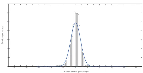
Figure 2: Empirical density of excess returns and the Normal PDF
−50 −40 −30 −20 −10 0 10 20 30 40 50
0 2 4 6 8 10 12 14
Excess returns (percentage)
D
en
si
ty
(p
er
ce
n
ta
ge
)
The figures reveal that stocks have consistently outperformed the risk-free security yielding
a monthly expected excess return (i.e., a equity premium) of 0.32%. However, stocks have
been riskier and this caused a high variability in U.S. excess returns over the same period,
with a monthly standard deviation of 4.08%.
In addition, Table 1 displays the statistics for the skewness and kurtosis - the third and
fourth standardized moments. Skewness and kurtosis are used to summarize the extent of
asymmetry and the tail thickness in a given empirical density distribution. For a Normal
distribution, these statistics correspond to 0 and 3, respectively. Therefore, it seems that the
Normal distribution does not hold for U.S. excess returns. Instead, the empirical distribution
of excess returns is leptokurtic, exhibiting a higher value of kurtosis (more than 14), and
asymmetric, with a negative skewness of −0.344. This conclusion holds true also for the
S&P500 index and the long-term U.S. Government Bonds.
Figure 2 plots an empirical density histogram against a theoretical Normal distribution.
The empirical density distribution of U.S. excess returns is more peaked in the center and
has fatter tails when compared to a Normal distribution. Overall, the Normal distribution
4
exhibits a very poor fit through all range of the data: at the center, frequencies are
sub-stantially underestimated; at a medium range from the center, the empirical frequencies
approach zero faster than the Normal alternative, i.e., they are overestimated; and, finally,
at the tails, empirical frequencies become again underestimated.
But how large is the error made if we assume a Normal distribution as a theoretical
model for U.S. excess returns? To quantify deviations from normality I build an empirical
frequency distribution of excess returns and compare it with what would be expected if the
same frequencies were calculated with a Normal distribution. The frequencies correspond
to the empirical proportions of excess returns within a given number of standard deviations
from the mean. I split the frequencies into three groups: Center, Medium and Tails. These
groups were chosen accordingly to the number of excess returns in the range of (µ±kσ), for
k∈Rand µ, σ are the sample mean and the sample standard deviation of excess returns.
Table 2: Excess returns: empirical frequencies vis-`a-vis Normal distribution
Position Range Observed Normal Difference
Center 0 to 1 79.05 68.27 10.78
Medium 1 to 3 19.40 31.46 -12.06
Tails 3+ 1.55 0.27 1.28
Left Tail 1.31 0.13 1.17
Right Tail 0.24 0.13 0.10
Empirical frequencies of excess returns and theoretical Normal frequencies. Range refers to the number of standard deviations beyond the mean. Column ”Difference” refers to the difference, in percentage, of empirical relative frequencies given in column ”Observed”, and the expected normal frequencies represented in column ”Normal”.
The magnitude of the deviations can be seen in Table 2. The first row of this Table
shows that the empirical distribution of excess returns contains 10.78% more observations
in the center than it would be expected if the distribution was Normal. The fact that a
large proportion of excess returns remains near its sample mean explains the higher peaked
frequencies are overestimated which, in Table 2, corresponds to the negative difference of
12.06%. However, the most important characteristic of empirical frequencies is the evidence
of two significant tails. A general observation about these extreme events is that 1.55% of
total excess returns correspond to more than three standard deviations from the mean. This
is about six times the value of the Normal distribution. Furthermore, the probability of
occurring extreme downward and upward movements in excess returns is not the same. In
Table 2, the left tail has a relatively higher density frequency which means that crashes are
more likely than booms. The Normal distribution, being a symmetric distribution, cannot
capture this feature.
2.3.3 Normality tests
In order to formally examining the normality assumption, I ran several classes of tests for
monthly excess returns. These tests have been widely used to study normality hypothesis
in empirical financial studies and they can be implemented in almost all standard statistical
packages. I carried out these tests using Eviews and Matlab.
The first test used is the Jarque-Bera test (Bera and Jarque,1987). This test uses
infor-mation on the third and fourth moments of a distribution and is based upon the fact that
for a Gaussian distribution, whatever its parameters, the skewness is 0 and kurtosis is 3.
The second test applied is the Shapiro-Wilk test (Shapiro and Wilk, 1965). This test
assumes that, under the null hypothesis, the data are coming from a Normal population with
unspecified mean and variance. This test is generally considered relatively more powerful
against a variety of alternatives. Shapiro-Wilk test is used, instead of Shapiro-Francia,
because it has a relatively better performance for leptokurtic samples.
Finally, I conducted three additional tests to get a more precise picture of normality: the
Anderson-Darling test (Stephens, 1974), the Lilliefors test (Lilliefors, 1967) and the
Cram´er-von-Mises test (Cram´er, 1928 and Anderson, 1962). These goodness-of-fit tests, which are
distribution and the Normal distribution using the sample estimated mean and variance.
Then, they assess whether that discrepancy is large enough to be statistically significant,
thus, requiring rejection of the Normal distribution under the null hypothesis.
Table 3: Normality tests in excess returns
Normality test Statistic value P-value
Jarque-Bera 9051.1 0.0000
Shapiro-Wilk 0.9030 0.0000
Anderson-Darling 20.696 0.0000
Lilliefors 0.0707 0.0000
Cram´er-von-Mises 3.1279 0.0000
Table 3 gathers the results of the normality tests performed in excess returns. All the
results point into the outright rejection of the normality assumption for U.S. monthly excess
returns.
According to the empirical literature, it is a “stylised fact” that distributions of stock
returns are poorly described by the Normal distribution (see Mandelbrot, 1963 and Campbell
et al., 1997). This empirical regularity was first reported by Mandelbrot (1963) when he
discovered fundamental deviations from normality in empirical distributions of daily returns.
More recently, Campbell et al. (1997) found contradictory evidence indicating that monthly
U.S. stock returns are reasonably well described by a Normal distribution. My results seem
to be closely related with Kim, Morley and Nelson (2005). They found that a Normal
assumption fails at capturing the distribution of monthly excess returns on a value weighted
NYSE portfolio during a smaller sample period (1926–1999). In particular, they found that
historical excess returns are characterized by higher statistical moments with a negative
3
Characterizing deviations from normality
So far I have found that normality does not hold for U.S. monthly excess returns. In
par-ticular, the empirical distribution of excess returns has long tails caused by a large kurtosis.
Now, I attempt to assess under which circunstances normality may be statistically acceptable
for U.S. excess returns.
When testing normality in the previous section I assumed - as many other financial
researchers did - independent and identically distributed (i.i.d.) excess returns and, therefore,
that the estimated parameters - mean and variance - remain constant for the entire sample
period. However, especially when long histories are being used, the stationarity hypothesis
may not hold: for the sample period under investigation, the parameters of the probability
distribution can be changing over time, experiencing shifts known as ”structural breaks”, or
switching among a finite set of values, that is, they are ”regime-switching”.
In this section, I explore those sources of deviations: structural breaks (subsection 3.1)
and regime switching (subsection 3.2) in monthly excess returns data. The existence of
structural breaks or regime switching may provide a solution to achieve normality for excess
returns conditional on subperiods or regimes, respectively.
3.1
Structural breaks
Structural breaks are low frequency shocks with a permanent - long run - effect which tend
to be related with significant economic and political events (Bai and Perron 1998, 2003).
In general, ignoring the presence of structural breaks may lead to misleading results.
First, structural breaks might cause unit root tests to loose their power. In such case,
one may, for instance, wrongly fail to accept stationarity for a given sample. In addition,
structural breaks can be seen as extreme events which are shown to contribution to the
leptokurtosis of financial returns. The degree of leptokurtosis, however, tends to disappear
simply estimating empirical models over subperiods. Finally, when structural breaks are
ignored, making inference about ordinary descriptive statistics, such as the mean or the
variance, may prove to be inaccurate. As referred by McConnel and Perez-Quiros (2000),
taking theory to the data by confronting the moments generated from a calibrated Normal
model with the moments of real data over a period with a structural break will lead to
misleading conclusions. Therefore, even if the normality assumption for excess returns is not
acceptable over the entire period, it could be so for subperiods between the breaks. That is,
the normality theory may still be valid conditional to those subperiods.
This subsection starts with a description of the methodology undertaken to test and date
structural breaks in monthly excess returns. Then, results are presented and normality is
tested again for excess returns using smaller periods.
3.1.1 Methodology
I follow a flexible approach that is capable of simultaneously test and date structural breaks.
It consists in a two-step procedure. In the first step, I use a generalized fluctuation framework
to test for the presence of breaks in the conditional mean and in the conditional variance
of excess returns. If there is evidence of breaks in the data, then, in the second step, I use
an algorithm from Bai and Perron (1998, 2003) for dating the potential breakpoints and
select the optimal number of breaks according to the Bayesian Information Criterion (BIC)
(Schwarz, 1978). Such approach was suggested by Hornik et al. (2003) and may be easily
implemented in their strucchange package for R software5.
A. Generalized fluctuation tests - first step
Structural breaks are permanent shifts that occur in the parameters of a data generating
process. Although structural breaks are detected by finding changes in the parameters of
a conditional model, they imply shifts in the unconditional moments. Following Hornik et
5
al. (2003), I consider the following standard linear regression model for testing parameter
stability,
yt =x
⊺
tβt+ut (t= 1, ..., T) (3.1)
whereyt is the observation of the dependent variable at timet,xt = (1, xt2, ..., xtk)⊺ is ak×1
vector of observations of the independent variables, ut is iid(0, σ2) and βt is a k×1 vector
of regression coefficients which may vary over time.
Under this set up we are concerned with testing the null hypothesis of ”no structural
change”
H0:βt = β0 (t= 1, ..., T) (3.2)
against the alternative that at least one coefficient vector varies over time.
To test this null hypothesis (are the parameters stable?), I use generalized fluctuation
tests. Generalized fluctuation tests fit a parametric model (3.1) to the data via ordinary least
squares (OLS) and derive an empirical fluctuation process which captures the fluctuation in
the residuals or in the coefficient estimates. The null hypothesis of parameter stability is
rejected if the fluctuation is considered improbably large.
I use two empirical fluctuation processes which are based in the estimates of regression
coefficientsβ: the recursive estimate (RE) process in the spirit of Ploberger et al. (1989) and
the moving estimate (ME) process introduced by Chu et al. (1995). From this point of view,
the k×1-vector β is either estimated recursively with a growing number of observations,
or using a moving data window of constant bandwidth h. For both RE and ME empirical
fluctuation processes, fluctuations are determined in terms of their deviations from the
full-sample estimate of the regression coefficient β.
These empirical fluctuation processes can capture departures from the null hypothesis
of parameter stability (3.2). In particular, the null hypothesis of ”no structural change”
should be rejected when the fluctuation of the empirical process becomes improbably large
corre-sponding limiting processes are known (see Kuan and Hornik, 1995) and, from these limiting
processes, boundaries can be found, whose crossing probability (under the null hypothesis)
is a prescribed significance critical rejection level α.
It should be noted, however, that generalized fluctuation tests are not a dating procedure
and a more general framework is needed to this purpose.
B. Dating multiple breakpoints - second step
Multiple breaks are likely to occur in long time series data. In such case, we may need
to consider a more general framework than the one considered in (3.1). According to Bai
and Perron (1998, 2003), it is assumed that there are m breakpoints and m+ 1 segments
(in which the regression coefficients are constant) and that the following multiple linear
regression model is given:
yt =x
⊺
tβ1+ut (t= 1, ..., T1),
yt =x
⊺
tβ2+ut (t=T1+ 1, ..., T2),
...
yt = x
⊺
tβm+1+ut (t=Tm+ 1, ..., T) ,
where the breakdates indexed by (T1, ..., Tm) are explicitly treated as unknown.
The main goal here is to determine the number and location of the breakpoints. That is,
we need to determine the estimates for them breakpoints and the m+ 1 segment - specific
regression coefficients βj+1, when T observations for (yt, xt) are available.
I estimate the breakpoints by applying the algorithm of Bai and Perron (2003) which was
recently implemented in R software by Hornik et al. (2003). The algorithm is based on the
principle of dynamic programming and it is considered, among others, one efficient method
The algorithm proceeds as follows. Given a fixed number of breakpoints, the algorithm
starts by calculating the sum of squared residuals for every possible segment in the regression
model. Some restrictions may be imposed to the number of segments to be calculated, such as
the minimum distance between each break. From all these possible segments, the algorithm
evaluates which partition - combination of segments - achieves a global minimization of the
overall sum of squared residuals. It is an iterative process solving a recursive problem and
from which the breakpoints, or equivalently the optimal partition, correspond to the global
minimisers.
For initialization, the algorithm requires a fixed number of breakpoints. In many
ap-plications, however, m is unknown and it must be chosen based on the observed data as
well. One solution to this problem is to compute the optimal segmentation for a sequence of
breakpoints m = 1,2,3, ...mmax and to choose m by optimizing some information criterion
(Bai and Perron, 2003). Model selection for the number of breakpoints m is based on the
minimization of BIC criteria. Further details on this algorithm can be found in Bai and
Perron (2003) and Hornik et al. (2003).
3.1.2 Tests results
A. Detecting evidence of structural breaks
This part reports the results for the structural break tests undertaken to the conditional
mean and the conditional variance of U.S. monthly excess returns. For each conditional
model two fluctuation tests have been carried out: the recursive estimates (RE) and the
moving estimates (ME). In the ME fluctuation tests, the moving date window of constant
bandwidth h was set up to 5%6.
Let the conditional mean of excess returns follow an autoregressive model of order 2
-AR(2). This model specification turns out to be necessary in order to remove autocorrelation
6
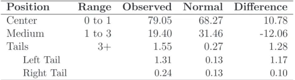
Figure 3: Stability tests in the conditional mean of excess returns
Recursive estimates test
Time
Empir
ical fluctuation process
0.0 0.2 0.4 0.6 0.8 1.0
0.0
0.5
1.0
1.5
Moving estimates test
Time
Empir
ical fluctuation process
0.0 0.2 0.4 0.6 0.8 1.0
0.0
0.2
0.4
0.6
0.8
1.0
1.2
Monthly, from 1871:01 to 2010:12. The empirical fluctuation process with the coefficient estimates are plotted together with its boundaries at an (asymptotic) 5% significance level.
Time refers to the fraction of the sample T.
from the residuals. Alternatively, we could assume a random walk model for the mean
of excess returns. Or we could use more sophisticated models with a higher number of
integration (e.g., AR(p) with p > 2). However, the empirical results remain qualitatively
the same. Thus, the standard linear regression model upon which the structural break tests
were based is,
yt =α+β1yt−1+β
2y
t−2+ǫt, ǫt ˜i.i.d N(0, σ
2) (3.3)
with yt the excess return in month t. Model (3.3) is a pure change model (Bai and Perron
1998, 2003) since all its regression coefficients - level α and persistence β - are allowed to
change.
Figure 3 reports the structural break tests for the conditional mean of U.S. monthly
excess returns. Clearly, the mean of excess returns did not vary much over the period. This
the boundary line of critical rejection of 5% and, hence, one may conclude that there are no
evidence of structural breaks in the mean of excess returns over the period from 1871:01 to
2010:12.
In order to run structural break tests in the variance, squared errors (ǫ2
t) taken from
equation (3.3) are considered as a proxy for the conditional variance of U.S. monthly excess
returns. Other proxies of volatility may be considered instead. One alternative is to estimate
a GARCH(1,1) model and work directly with the equation of conditional volatility. Or we
may simply calculate the sample volatility using a moving data windows.
Let the conditional variance of excess returns follow an autoregressive model of order
1 - AR(1). Again, this model specification turns out to be necessary in order to remove
autocorrelation from the residuals. Alternatively, we could assume a random walk model for
the mean of excess returns. Or we could use more sophisticated models with a higher number
of integration (e.g., AR(p) with p≥2). However, the empirical results remain qualitatively
the same. Thus, the standard linear regression model upon which the structural break tests
were based is,
ǫ2t =δ+ηǫ2t−1+ζt with ζt ˜i.i.d N(0, σ2). (3.4)
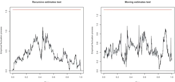
The results, displayed in Figure 4, appear to be rather different for the conditional
vari-ance of U.S. monthly excess returns. At a 5% (asymptotic) significvari-ance level, both empirical
fluctuation processes show significant departures from the null hypothesis of parameter
sta-bility, suggesting the existence of a structural break for the variance of excess returns.
Yet the number of breaks seems to be different across the tests: whereas the RE test
points to one peak, the ME test depicts two - or possibly three - peaks where the fluctuation
of the empirical process is improbably large compared to the fluctuation of the limiting
process under the null hypothesis. Therefore, it seems that there is more than one structural
Figure 4: Stability tests in the conditional variance of excess returns
Recursive estimates test
Time
Empir
ical fluctuation process
0.0 0.2 0.4 0.6 0.8 1.0
0.0
0.5
1.0
1.5
2.0
2.5
Moving estimates test
Time
Empir
ical fluctuation process
0.0 0.2 0.4 0.6 0.8 1.0
0.0
0.5
1.0
1.5
2.0
2.5
Monthly, from 1871:01 to 2010:12. The empirical fluctuation process with the coefficient estimates are plotted together with its boundaries at an (asymptotic) 5% significance level.
Time refers to the fraction of the sample T.
B. Dating the breakpoints
After having found evidence of structural changes in the variance of excess returns, now
I attempt to answer the question of when they have occurred. For dating the breakpoints
an algorithm from Bai and Perron (1998, 2003) has been applied to the conditional variance
model (3.4).
However, there are two important practical issues that we should take into account when
applying the algorithm. One is related to the number of breaks to be considered in the
dating procedure. I assume a maximum ofm= 5 potential structural breaks and then select
m according to a model selection which is based on the BIC criteria. Furthermore, I set
up a minimum segment size of 96 months, corresponding to 5% of the 1871-2010 sample.
According to Kim et al. (2005), this procedure turns out to be necessary to avoid any
irregularities in the likelihood function resulting from a small subsample. Moreover, under
this particular methodology, I am looking for permanent – rather than temporary – shifts in
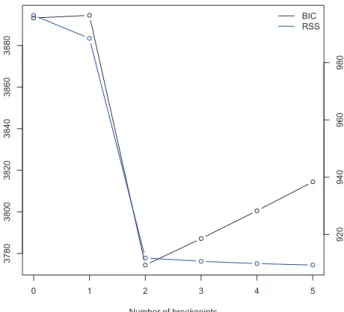
Figure 5: BIC (and RSS) values for different number of breakpoints.
0 1 2 3 4 5
3780
3800
3820
3840
3860
3880
BIC and Residual Sum of Squares
Number of breakpoints
BIC RSS
920
940
960
980
time7.
Figure 5 displays the BIC criteria for models estimated up to m = 5 structural breaks.
The BIC criterion selects two breakpoints for the variance of U.S. monthly excess returns.
Looking at Figure 5, we may conclude that the value for which BIC is minimised is atm= 2.
The Residual Sum of Squares (RSS) may be considered as an alternative information criterion
for model selection. RSS, however, is monotonically decreasing suggesting a model with a
higher number of breakpoints. Even though, I maintain my prior methodology to select
structural breaks according to BIC criterion.
Table 4: Breakdates found in the conditional variance of excess returns
Breakdates estimates
mTˆ1 1929:06
mTˆ2
1938:07
7
Table 4 reports the corresponding breakdates for the model withm= 2 structural breaks.
Breakdates for the variance of U.S. monthly excess returns were found at 1929:06 and 1938:07.
These dates are related with the Great Depression in the late 1920s and the beginning of
World War II.
These findings are somehow related with previous literature. Kim et al. (2005) found
evidence of a structural break in U.S. monthly excess returns around the WWII period.
In particular, this structural break is found to be associated with a permanent reduction
in the general level of stock market volatility. My methodology finds support of breaks in
the variance but not in the mean of excess returns. However, I found one additional break
around the Great Depression period. Since Kim et al. (2005) studied a shorter sample period
1926-1999 and have set a wider length for each segment (10%), this may explain, in part,
why they only found one – instead of two – structural break(s).
P´astor and Stambaugh (2001) reported a larger number of structural breaks for expected
U.S. monthly excess returns (15 in total) over a longer sample period (1834-1999). The most
significant break, however, was found to be in the late 1990s. In my procedure, I specify
only 5 potential breaks. I also tried higher values for the maximum number of breaks to be
considered but the findings were similar. Moreover, my model selection procedure is based
on BIC criterion which rules out complex models (with a high number of segments), thus,
favouring parsimony.
3.1.3 Normality in different subperiods
Breakdates for the variance of U.S. monthly excess returns were found at 1929:06 and 1938:07.
This implies a model for the variance of excess returns with three subperiods. In this part, I
assess normality for monthly excess returns over three subperiods: the first covering the time
period until 1929:06, the second including the Great Depression period, starting in 1929:07
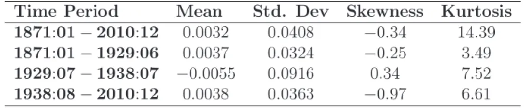
Table 5: Descriptive statistics for excess returns over different periods
Time Period Mean Std. Dev Skewness Kurtosis 1871:01−2010:12 0.0032 0.0408 −0.34 14.39
1871:01−1929:06 0.0037 0.0324 −0.25 3.49
1929:07−1938:07 −0.0055 0.0916 0.34 7.52
1938:08−2010:12 0.0038 0.0363 −0.97 6.61
Table 5 reports the descriptive statistics for monthly excess returns for the whole sample
period as well as for three different subperiods. There are several important findings in Table
5. First, excess returns during the Great Depression (second subperiod) were negative and
extremely volatile. The average of excess returns during this subperiod was −0.55% with a
standard deviation of more than 9.16%, which is almost three times higher than that for the
other subperiods.
Second, normality in excess returns depends on the sample period over which data is
observed. The subperiod before the Great Depression seems to be consistent with normality.
For this subperiod, excess returns reveal a kurtosis of 3.49 and a slightly negative skewness
of −0.25. On the other hand, normality is still not a reasonable assumption for the other
two subperiods. The statistics for these two time spans reveal that the second subperiod
exhibits the highest kurtosis (7.52) while the latter subperiod has the lowest value of skewness
(−0.97).
Third, deviations from normality in excess returns for the three subperiods are smaller
than those for the whole sample period. Looking at Table 5, the degree of leptokurtosis,
in particular, is far less evident for the three subperiods when compared to the full-sample
period. Therefore, it seems that the presence of structural breaks can, in part, explain the
excess kurtosis for excess returns.
3.2
Regime Switching
The stationarity hypothesis may not hold due to the existence of structural breaks but also
changes as opposed to changes of a recurring nature which can be rather captured by regime
switching models. In the latter, the parameters move and then revert from one regime to
the other.
There are two different approaches for modelling regime switching. One approach uses
Markov switching models, which define a probability transition matrix governing the shifts
between regimes in a conditional regression model. A rather different approach uses a discrete
mixture of distributions to fit the unconditional empirical distribution. Typically, two or
three (or a finite number of) density distributions are defined, representing quiet and more
turbulent regimes.
The purpose of this section is to find for market regimes in U.S. monthly excess returns.
This is accomplished by estimating Normal mixture models up to G = 5 regimes for the
excess returns data. Overall, it has been argued that the true distribution of stock returns
may be Normal, although its parameters are ”regime-switching” (Kon, 1984). In this sense,
normality for excess returns may hold conditionally whether the data is arising from different
market regimes.
I start this section by presenting the Gaussian mixture model and explaining the
Expectation-Maximization (EM) algorithm (Dempster et al. 1977) used for the estimation of such model.
Then, I report the estimation results for the excess returns in the sample period spanning
from 1871:01 to 2010:12. Finally, using post WWII data, I assess if the Gaussian mixture
model provides a reasonable model for the empirical distribution of monthly excess returns.
3.2.1 Gaussian mixture model
The Gaussian mixture distribution has been widely used as a suitable alternative for
mod-elling distributions of financial returns. Gaussian mixture models as models for distributions
of returns were first suggested by Kon (1984). This author proved that discrete mixture
of Normal distributions can in fact explain both significant kurtosis (fat tails) and positive
mixtures of Normal distributions have the advantage of maintaining the tractability of a
Normal distribution: the unconditional mean and variance are simply expressed as a linear
combination of means and variances of different regimes.
Let g = 1, ..., G be the components, or equivalently the regimes, of the mixture model
and consider that each component has a Normal density φ x;µg, σg2
with unknown means
µ1, ..., µG and unknown variances σ21, ..., σ2G. Under these circumstances, excess returns xt
are said to have density described by a finite mixture of Normal distributions,
f (x; Ψ) =
G
X
g=1
πgφ x;µg, σg2
(3.5)
where πg is the (a priori) probability of an observation xt belonging to the g−th regime
and Ψ includes θ= (µ1, ..., µG, σ12, ..., σG2) and the probabilities π1, ..., πG for G regimes.
The two main goals are: (i) to estimate the vector Ψ of unknown parameters and (ii) to
select the number of regimes G. To do so, I apply a flexible two-step approach. In the first
step, I estimate the parameters of Normal mixture models with a fixed number of regimesG
using the Expectation-Maximization (EM) algorithm (Dempster et al. 1977). In the second
step, I select the number of regimes G according to the Bayesian Information Criterion
(Schwartz, 1977). Such approach has been shown to achieve a good performance to select
the number of regimes in several applications (see Dasgupta and Raftery 1998) and it may
be easily implemented in the MCLUST package forR software (Dasgupta and Raftery, 1998
and Fraley and Raftery, 1999 and 2002).
3.2.2 Expectation-maximization
Maximum-likelihood (ML) estimates for the parameters of Normal mixtures cannot be
written down in a closed form (Titterington, 1996); instead, these ML estimates have to
be computed iteratively. I estimate the parameters of Normal mixture models using the
Expectation-Maximization (EM) algorithm (Dempster et al. 1977).
estimation problems involving incomplete data, or in problems which can be posed in a
similar form, such as the estimation of finite mixtures distributions. In particular, for
the purpose of the application of the EM algorithm, the observed-data vector of excess
returns x = (x1, ..., xn) is regarded as being incomplete; that is, we do not know which
mixture component underlies each particular observation. Therefore, any information that
permits classifying observations to components should be included in the mixture model.
The component-label variables zt = (zt1, ..., ztG) are consequently introduced, where ztG is
defined to be one or zero according to ifxt did or did not arise from the G−th component
of the mixture model, respectively. Moreover, if zt is i.i.d. with a multinomial
distribu-tion of one draw from G categories with probabilities π1, ..., πG, we may represent the new
complete-data loglikelihood for excess returns as
l(θg, πg, ztg|x) =Pnt=1PGg=1ztglog [πgf(xt|θg)],
where the values ofztg are unknown and treated by the EM as missing information on
to be estimated along with the parameters θ and π of the mixture model.
The EM algorithm starts with some initial guess for the parameters in the mixture
ˆ
Ψ (component means ˆµg, component variances ˆσg2 and mixing proportions ˆπg). Based on
such guessed values, the algorithm finds the ML estimates by applying iteratively until
convergence the expectation step (E-step) and the maximization step (M-step).
The E-step consists, at iteration h, in computing the expectation of the complete data
loglikelihood over the unobservable component-label variablesz, conditional on the observed
data xt and using the current estimates on the parameters ˆΨ(h),
ˆ
τtg(h)=Ehztg|xt; ˆΨ(h)
i =
ˆ
πg(h)φ
xt; ˆθ(
h)
g
PG
g=1ˆπ (h)
g φ
xt; ˆθ(
h)
g
,
for g = 1, ..., Gand t= 1, ..., n. Note that ˆτtg(h) is the estimated posterior probability (at
In the M-step, new parameters ˆΨ(h+1)are obtained by maximizing the expected complete
data loglikelihood. These new parameters are estimated from the data given the conditional
probabilities ˆτtg that were calculated from the E-step. Estimates of πg and θg have simple
closed-form expressions involving the data and ˆztg from the E-step.
Once we have a new generation of parameter values ˆΨ(h+1), we can repeat the E-step
and another M-step. The E and M-steps are alternated repeatedly until the likelihood (or
the parameter estimates) change by an arbitrarly small amount in the case of convergence.
The EM algorithm increases the likelihood function of the data at each iteration, and under
suitable regularity conditions converges to a stationarity parameter vector.
3.2.3 Number of regimes
When Normal mixture models and its corresponding parameters have been estimated, the
number of regimes to consider in excess returns has to be decided. I assume a standard
statistical problem in which the number of regimes G is known, but mixture models with
different G should be compared based on some type of information criterion.
I select the number of regimesG according to the Bayesian Information Criterion (BIC)
(Schwarz, 1978). The BIC chooses G to minimize the negative loglikelihood function
aug-mented by some penalty function which rules out complex models with a large number of
parameters. Overall, parsimony-based approaches have been proposed for choosing the
op-timal number of regimes in a given mixture model. In particular, Bayesian Information
Criterion (BIC) has been shown to achieve a good performance to select the number of
regimes in several applications (see Dasgupta and Raftery 1998). Medeiros and Veiga (2002)
proposed a rather different approach to select the number of regimes in financial volatility.
In such approach, the problem of selecting the number of regimes is solved by applying
3.2.4 Parameter estimates
In summary, the following strategy for model selection has been performed: (i) a maximum
number of regimes, Gmax is considered; (ii) then, the parameters are estimated via EM for
each model with a number of regimes up to Gmax; (iii) BIC is compared for each model; and
(iv) finally, the number of regimes is selected such as to minimise BIC8.
A. Full sample period
This part reports the results from the application of MCLUST package to monthly excess
returns data from 1871:01 to 2010:12. Mixtures up to G = 5 Normal distributions were
estimated via EM algorithm for monthly excess returns over the period 1871:01 to 2010:12.
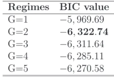
Table 6: BIC values for different numbers of regimes in excess returns
Regimes BIC value
G=1 −5,969.69
G=2 −6,322.74
G=3 −6,311.64
G=4 −6,285.11
G=5 −6,270.58
Table 6 presents the corresponding BIC value calculated for each Normal mixture model.
There are two regimes in U.S. monthly excess returns. Looking at Table 6, the mixture model
for which the BIC value is minimised is atG= 2. Furthermore, the stationary Normal model
with G = 1 has the worst performance among all the models. Hence, it seems that excess
returns over the period from 1871:01 to 2010:12 may be described by a combination ofG = 2
Normal distributions. The corresponding maximum likelihood estimators for the parameters
are
8
fGM(x; ˆπ1,ˆπ2,µˆ1,µˆ2,σˆ1,σˆ2) = 0.9021·φ(x; 0.0066,0.0009) +
+ 0.0979·φ(x;−0.0286,0.0078) (3.6)
The density model for excess returns in (3.6) reflects the existence of two market regimes:
the first density, occurring with a probability of 90%, may be interpreted as a bull market
regime - corresponding to months where excess returns have a relatively higher mean and a
smaller variance - whereas the second density, occurring with a probability of 10%, may be
interpreted as a bear market regime - corresponding to months where excess returns have a
lower expected return and a greater variance.
One attractive property of mixture models compared to a stationary Gaussian model is
that they can capture the leptokurtic and skewed characteristics of empirical data (Kon,
1984). To illustrate this flexibility, consider the probability density function of U.S. monthly
excess returns in (3.6). Leptokurtosis arises from a relatively larger variance in regime 2
occurring with probability 10% which enables the mixture to put more mass at the tails.
However, the majority of excess returns (90%) are coming from regime 1. Since this regime
contains data which is expected to be closer to the (unconditional) sample mean this,
there-fore, explains the high peak observed in the empirical distribution of excess returns. On the
other hand, skewness arises when means are different between regimes. In particular, there
is a negative asymmetry in the density model (3.6) since the high–variance regime has both
a smaller mean and a smaller mixing weight.
B. Post-WWII data
I have already found deviations from normality in U.S. monthly excess returns over the
subperiod from 1938:08 to 2010:12. Now, I investigate if those deviations arise from regimes
changes. That is, I test the viability of Normal mixture models as a descriptive model for
Figure 6: Empirical density of excess returns and the PDF mixture of two Normal distribu-tions
−25 −20 −15 −10 −5 0 5 10 15 20 25 0
2 4 6 8 10 12 14 16
Excess Returns (percentage)
D
en
si
ty
(p
er
ce
nt
ag
e)
Table 7: BIC values for different number of regimes in excess returns over post-WWII data
Regimes BIC value
G=1 −3,286.63
G=2 −3,375.42
G=3 −3,359.05
G=4 −3,344.23
G=5 −3,330.53
Table 7 reports the BIC value for mixtures up toG = 5 Normal distributions estimated
via EM algorithm for U.S. monthly excess returns over the period 1938:08 to 2010:12. Again,
there are two regimes in U.S. monthly excess returns. The BIC criterion selects a model
with G = 2 and, therefore, a mixture of two Normal distributions may be considered as a
relatively good descriptive model to explain U.S. monthly excess returns over the subperiod
from 1938:07 to 2010:12. In contrast, the stationary Normal model withG= 1 has the worst
performance among all the models.
Figure 6 plots empirical density histograms for U.S. monthly excess returns together
with a density of a mixture of two Normal distributions over the subperiod from 1938:07 to
for U.S. monthly excess returns. Looking at Figure 6, it is particularly evident that the
combination of two Normal distributions can capture the larger peakness and the heavier
tails revealed in the empirical distribution of excess returns.
In this section, I found evidence of two regimes with different means and variances for U.S.
monthly excess returns and, at least for the last 70 years, these regimes can explain, in part,
deviations from normality for this particular subperiod. These findings may be somehow
related with the previous literature. Kim et al. (2005) compared four univariate models of
monthly excess returns over the period 1926-1999 and they found that the three models that
incorporate Markov switching volatility are preferred over the simple i.i.d. model.
There is a wide empirical evidence, in the literature, for the existence of regimes in stock
returns. Kon (1984) examined daily returns of 30 stocks of the Dow Jones and estimated
mixtures of Gaussian distributions with two up to four regimes which were found to fit
ap-propriately. Aparicio and Estrada (1995) found partial support for a mixture of two Normal
distributions to explain the distributions of stock returns of 13 European securities markets
during 1990-1995 period. Using monthly S&P 500 stock index returns (1871–2005), Behr
and P¨otter (2009) investigate the viability of three alternative parametric families to
repre-sent both the stylised and empirical facts and they have concluded that the two component
Gaussian mixture has the smallest (maximal absolute) difference between empirical and
es-timated distribution. They have suggested that, given its flexibility and the comfortable
estimation using the EM algorithm, Gaussian mixture models should be considered more
frequently in empirical financial analysis.
4
Time aggregation and Normality
I found consistent deviations from normality in monthly excess returns for the post-WWII
data. These deviations were associated with regime switching. Since normality is a key
theoret-ical asset pricing, should we consider most of finance theory as unrealistic, and, therefore,
irrelevant? That is, should we abandon normality for this particular subperiod? In this final
section, I assess under which circumstances normality of excess returns may be reconsidered
for the post-WWII data.
My main emphasis here is to see whether Gaussianity for excess returns depends or
not on the frequency of the data. This is equivalent to test for aggregational Gaussianity.
Aggregational Gaussianity means that as one increases the time interval over which returns
are calculated, their distribution looks more and more like a Normal distribution. Therefore,
normality in excess returns may not hold for high frequency data - up to monthly data - but
it may hold for higher aggregate data.
In order to test aggregational Gaussianity for U.S. excess returns, I use post-WWII data
measured at different time intervals. Ultimately, I try to determine the level of aggregation
for which excess returns converge to a Normal distribution.
This section starts with a brief description of the data. Then, I test for the aggregational
Gaussianity for U.S. excess returns. This section ends with some formal normality tests.
4.1
Data
I use excess returns data measured over daily, weekly, monthly, quarterly, semi-annual and
annual frequencies for the sample period starting at 01/08/1938 until 31/12/2010. I use
end-of-period data for all frequencies. From end-of-day figures, I calculate end-of-week excess
returns when 7 calendar days are available. Similarly, using the last day of each month, I
compute monthly excess returns. For quarterly excess returns, I assume, for each year, the
end-of-month observation in March, June, September and December. Semi-annual
observa-tions are the end-of-month figure in June and December and, finally, annual observaobserva-tions
correspond to the last day of each year.
The data sources are as follows. For stock prices, I use daily quotes from Bloomberg for
Figure 7: Empirical density of excess returns and the Normal PDF for different levels of aggregation
−30 −20 −10 0 10 20 30
0 1 2 3 4 5 6 7
Excess Returns (percentage)
D en si ty (p er ce n ta g e)
(a) Daily Frequency
−30 −20 −10 0 10 20 30
0 2 4 6 8 10 12 14
Excess Returns (percentage)
D en si ty (p er ce n ta g e)
(b) Weekly Frequency
−30 −20 −10 0 10 20 30
0 4 8 12 16 20 24
Excess Returns (percentage)
D en si ty (p er ce n ta g e)
(c) Monthly Frequency
−40 −30 −20 −10 0 10 20 30 40 0 5 10 15 20 25 30 35
Excess Returns (percentage)
D en si ty (p er ce n ta g e)
(d) Quarterly Frequency
−40 −30 20 10 0 10 20 30 40
0 5 10 15 20 25 30 35 40
Excess Returns (percentage)
D en si ty (p er ce n ta g e)
(e) Semi-annual Frequency
−0.6 −0.4 −0.2 0 0.2 0.4 0.6 0 10 20 30 40 50
Excess Returns (percentage)
D en si ty (p er ce n ta g e)
(f) Annual Frequency
and weekly observations, I apply linear interpolation to monthly data. For the risk-free asset,
I use yields from the 3-month Treasury Bills published by Federal Reserve. In particular:
(i) for daily and weekly frequencies and up to 04-01-1954, I use monthly observations which
are linear interpolated to obtain daily and weekly observations (ii) for the remaining period,
I use daily observations of the 3-month Treasury Bill secondary market rate (yield).
4.2
Aggregational Gaussianity
A simple way to check normality is to plot the empirical density histogram against the
theoretical Normal distribution with the same empirical moments - mean and variance.
Figure 7 reports empirical distributions of excess returns recorded over time intervals
Figure 7 is the fit of a Normal distribution with a mean and variance given by the respectively
empirical moments.
There is evidence of aggregational Gaussianity in U.S. excess returns. Visual inspection of
the empirical distributions suggests that these distributions are high-peaked and leptokurtic
for lower levels of aggregation (up to quarterly data). However, the peak sharpness and
the extent of leptokurtosis in the empirical distributions seem to decrease substantially and
become more Gaussian-like as we move for higher levels of aggregation. Overall, normality
seems to be a reasonable assumption for excess returns for frequencies starting at semi-annual
data. At this level of aggregation, the shape of the empirical distribution of excess returns
is closer to the bell-shape of the Gaussian distribution. In particular, the corresponding
empirical distribution is characterized by thinner tails and a less peaked center compared to
the empirical distributions for the lower levels of aggregation and, thus, it is more similar to
the Gaussian benchmark.
Table 8: Descriptive statistics for excess returns over different time levels of aggregation
Time frequency Mean Std. Dev. Skewness Kurtosis
daily 0.0002 0.0117 -0.34 22.29
weekly 0.0012 0.0212 -0.66 9.03
monthly 0.0051 0.0440 -0.83 6.37
quarterly 0.0155 0.0806 -0.90 4.65
semi-annual 0.0308 0.1171 -0.46 3.28
annual 0.0624 0.1711 -0.77 3.82
The most evident fact about excess returns data is that as the level of aggregation
increases so the kurtosis falls. Looking at the Table 1, the kurtosis coefficient is widely
above 3 for daily frequencies, it slowly decreases up to the quarterly frequency and, finally, it
reaches convergence to normality at semi-annual and annual frequencies. Skewness statistics
do not yield a consistent pattern. These statistics suggest that excess returns are negatively
skewed but this is not a major feature for these data. In addition, the higher the level