M
ESTRADO
M
ATEMÁTICA
F
INANCEIRA
T
RABALHO
F
INAL DE
M
ESTRADO
D
ISSERTAÇÃO
D
YNAMICS OF
F
INANCIAL
M
ARKETS
:
S
TUDY OF AN
A
GENT
-
BASED
M
ODEL
J
OÃO
F
RANCISCO
M
AGRO
M
ARQUES
M
ESTRADO EM
M
ATEMÁTICA
F
INANCEIRA
T
RABALHO
F
INAL DE
M
ESTRADO
D
ISSERTAÇÃO
D
YNAMICS OF
F
INANCIAL
M
ARKETS
:
S
TUDY OF AN
A
GENT
-
BASED
M
ODEL
J
OÃO
F
RANCISCO
M
AGRO
M
ARQUES
O
RIENTAÇÃO
:
J
OSÉ
P
EDRO
R
OMANA
G
AIVÃO
Over the past few decades, the global financial market has been facing multiple distresses and crashes which led to troubled years for the real economy and families. Dynamical systems emerged in the mathematical finance literature to help comprehending better the unique characteristics of these financial markets and the price dynamics over the time. This work consists mainly of a statistical approach of the one discontinuity point dynamical system market model introduced by Tramontana, Westerhoff and Gardini (2010). Using a model’s version that produces chaotic orbits, we can observe stationary distributions under specific parameters. In other words, the dynamical system can be chaotic in a point-wise perspective, however, from a statistical approach, it can be asymptotically predictable, that is, most trajectories converge to an attractor which we can describe statistically. Still, under the proper parameters, the model may project an absolute erratic behavior, even in the statistical approach sense. For the latter, we conclude the price forecast is impossible because we can only restrict our prognoses to an invariant set sufficient large whose contain the whole price dynamic.
Nas ´ultimas d´ecadas, o mercado financeiro mundial tem enfrentado v´arios problemas e colapsos que motivaram anos conturbados para a economia real e para as fam´ılias. Os sistemas dinˆamicos apareceram na literatura de matem´atica financeira para ajudar a com-preender melhor as caracter´ısticas ´unicas destes mercados financeiros e a dinˆamica do pre¸co ao longo do tempo. Este trabalho consiste principalmente numa aproxima¸c˜ao es-tat´ıstica ao sistema dinˆamico de modelo de mercado com um ponto de descontinuidade introduzido por Tramontana, Westerhoff e Gardini (2010). Usando uma vers˜ao do modelo que produz ´orbitas ca´oticas, podemos observar, para parˆametros espec´ıficos, distribui¸c˜oes estacion´arias. Por outras palavras, o sistema dinˆamico pode ser ca´otico do ponto de vista do estudo das ´orbitas, por´em, em termos estat´ısticos, ´e assintoticamente previs´ıvel, isto ´e, a maioria das trajet´orias converge para um atractor que n´os conseguimos descrevˆe-lo estatisticamente. Ainda, para os parˆametros apropriados, o modelo pode projetar um comportamento absolutamente err´atico, mesmo numa aproxima¸c˜ao estat´ıstica. Para este ´
ultimo, n´os conclu´ımos que a previs˜ao do pre¸co ´e imposs´ıvel uma vez que s´o conseguimos restringir os nossos progn´osticos a um intervalo invariante suficientemente grande que cont´em toda a dinˆamica do pre¸co.
Em primeiro lugar, quero agradecer ao meu orientador Professor Doutor Jos´e Pedro Gaiv˜ao pela not´avel supervis˜ao e empenho incondicional. Estou grato por ter tido a oportunidade de trabalhar com um dos melhores professores de matem´atica que eu j´a conheci. Tamb´em quero agradecer-lhe por me ter proposto um tema muito interessante, nomeadamente numa ´area da matem´atica com a qual n˜ao estava muito familiarizado, mas que fui aprendendo a gostar.
Quero tamb´em agradecer `a minha fam´ılia, especialmente `a minha m˜ae e ao meu pai, pelo apoio que me deram para continuar os meus estudos. Foram sem d´uvida uma fonte de motiva¸c˜ao para levar esta etapa acad´emica at´e ao fim.
1 Introduction 1
2 One-Dimensional Dynamical Systems 3
2.1 Linear and Nonlinear Systems . . . 3
2.2 Semidynamical and Dynamical Systems . . . 4
2.2.1 Iterated Maps and Semiflow . . . 4
2.2.2 Trajectories and Orbits . . . 4
2.2.3 Semidynamical Systems . . . 5
2.2.4 Dynamical Systems . . . 5
2.3 Explicit Solutions . . . 6
2.4 Stationary Behavior . . . 6
2.4.1 Fixed Points and Stationary States . . . 6
2.4.2 Existence of Stationary States . . . 6
2.5 Cycles . . . 7
2.6 Stability Theory . . . 7
2.6.1 Stable, Asymptotically Stable and Unstable . . . 7
2.6.2 Expansivity . . . 8
2.7 Chaos: an Informal Perspective . . . 9
3 Statistical Dynamics 10 3.1 The Recurrence Theorem . . . 11
3.2 Limit Sets and Attractors . . . 12
3.3 Ergodic Dynamical Systems . . . 12
3.4 Distributions for Dynamical Systems . . . 13
3.4.1 Absolute Continuity: Density and Distribution . . . 13
3.4.2 The Number of Absolutely Continuous Invariant Ergodic Measures . 15 3.4.3 The Mean and Variance of a Trajectory . . . 15
3.5 Constructing Densities . . . 15
3.5.1 The Frobenius-Perron Operator . . . 16
3.6 Other Statistical Properties . . . 17
4 Dynamics of Lorenz Maps 19 5 Applications: a Simple Financial Market Model 24 5.1 Setup with One Discontinuity Point . . . 25
5.2 Bounded Instability Regime . . . 27
5.3 Symmetric Speculator Behavior . . . 30
5.4 Extreme Cases of Symmetric Speculator Behavior . . . 32
6 Discussion and Conclusions 33 Appendix 34 A.1. Example 2.2 - Strictly Monotonic System . . . 34
A.2. Proof of Corollary 2.1 . . . 35
A.3. Proof of Theorem 2.2 . . . 35
A.4. Proof of Proposition 3.1 . . . 36
A.5. Proof of Theorem 3.2 . . . 37
A.6. Proof of Proposition 3.2 . . . 38
A.7. Example 3.4 - Invariant Density Function . . . 39
A.8. Example 3.4 - MATLAB Code for the Empirical Approach . . . 41
A.9. Proof of Lemma 4.3 . . . 42
A.10. Proof of Proposition 4.1 . . . 42
A.11. Proof of Lemma 5.3 . . . 43
A.12. Proof of Lemma 5.4 . . . 44
1
Introduction
After the Great Depression (1929), some economists1 didn’t believe that was possible
to experiment another financial crisis with such noxious and wicked consequences to the global economy and the mankind. Nevertheless, the exponential growth of technology and the fast development of emerging economies establish new demanding challenges to the global financial system. Over the last four decades, financial market flaws became more frequent and severe, jeopardizing the real economy. The first (1973) and the second Oil crisis (1979), the Black Wednesday (1992), the Asian financial crisis (1997), the Dot Com bubble (2000) and the Subprime crisis (2008) are a few remarkable examples of recent global financial disasters with catastrophic outcomes at a global scale.
Past experience gives some vague clues about the causes of financial crises. Just before a market crash, the price for a certain asset keeps growing, but, at some point, the market is no longer willing to keep paying more for that asset and then the price drives in a free falling. Such price dynamics is called bull-bear market dynamic. Bull markets are optimistic periods when prices are generally rising. On the other hand, bear markets are associated with pessimistic periods when prices are generally falling. It’s also important to consider that in financial markets there is a very wide amount of participants, each one with his own perception of the market and reaction to the available information. The more the multiplicity and heterogeneity of the participants, the more unpredictable is the variation of the market prices. This complex behavior must be taken into account when designing mathematical models to forecast bull and bear dynamics, since participant’s actions interfere direct or indirectly in the price of the assets.
The introduction of this kind of models had been made by Day and Huang (1990) [6], when they presented a simple one-dimensional nonlinear system with three market participants:
❼ Chartists - the noise traders; they believe in the persistence of bull or bear markets;
❼ Fundamentalists - they bear the price convergence to the fundamental price of the asset2;
❼ Market maker - he adjusts the price according to the law of supply and demand.
This model absorbs the actions made by the participants changing the price dynamics in an unpredicted way (the price in the next period, sayn+ 1, can increase or decrease). Bull and bear markets may appear and then we can measure how likely financial stress events emerge. Huang and Day (1993) [12] modified their initial work and created an one-dimensional continuous linear model to approach this issue. They have to assume the fundamentalists are only willing to play in the market if the difference between the asset price and his fundamental exceeds a certain critical value. Afterwards, several papers and publications regard this matter come to light. Even with simple linear systems, it’s
1See Krugman (2009) [14].
possible to check some stylized facts from financial markets and the randomness of the asset price evolution. Hence, these kind of models became important in the mathematical finance literature.
For the purposes of this thesis we are going to discuss the work which we believe that led to a good improvement of the models developed by Day and Huang. Tramontana et al (2010) [18] generalized the financial models introduced by Day and Huang (1990) [6] and Huang and Day (1993) [12] using piecewise systems rather than nonlinear or continuous linear systems: the paper uses a model with one discontinuity point to approach this issue. For each investment philosophy, the authors decided to split the market investors in two types:
❼ Type 1 - always active in the market, no matter the price of the asset;
❼ Type 2 - only active in the market if the price of the asset is above or below a certain critical value.
Across to the analysis of these financial models, we need to bring out some definitions and results from dynamical systems applied to the one-dimensional space R. Dynamical systems play a crucial role on approaching problems related to the real economy and financial markets. As a consequence, they are essential and the core of this thesis.
2
One-Dimensional Dynamical Systems
2.1 Linear and Nonlinear Systems
Definition 2.1. Consider a map(function)θ:D→D, where Dis a close interval in R
like [a, b]or D is the whole set R. Then xn+1 =θ(xn) is a first-order difference equation.
The pair (θ, D) is called a system.
Example 2.1. We introduce some functions that can be used to define θ or that are in-volved in the derivation of mapθfor many cases. The domain sets are just demonstrative.
Affine system:
θ(x) =ax+b, D=R, a, b∈R (2.1a)
Quadratic system:
θ(x) =α+βx+γx2, D=R+0 and α, β, γ∈R (2.1b)
Piecewise linear system: let a0, ..., an, b0, ..., bn, be sequences of real numbers with
ai−1 < ai, i= 1, ..., n. Then D:= [a0, an] and:
θ(x) =bi+βi(x−ai), ai ≤x≤ai+1, (2.1c)
whereβi = (bi−bi−1)/(ai−ai−1) = 1, ..., n. θcombinesnlinear (affine) segments that are
joint to form a continuous map on the interval [a0, an]. Nevertheless,θ may be also built withnlinear segments to define a discontinuous map on [a0, an] with continuous branches on each [ai, ai+1].
Definition 2.2. Let (θ1, D1) and(θ2, D2) be two systems. If there exists a bijective
func-tionh:D1→D2 such that θ2◦h=h◦θ1, thenθ1 andθ2 are conjugatedand h is called
the conjugationwhich is represented by the following diagram:
D1 D1
D2 D2
θ1
h h
θ2
In a non-theoretical environment, specific formulas as we introduce in the previous example are quite rare. They basically appear for illustration purposes. Fortunately, in most cases it is possible to derive the behavior of a system based exclusively on its qualitative properties. In terms of empirical work and forecasting, qualitative estimates are the best tools available and are also sufficiently powerful.
A class of systems with broadly application to economics and finance is the following:
Definition 2.3. A map θ defined on D ismonotonic if for allx, y∈D either:
In the first (second) case, θ is monotonic increasing (decreasing). The map is strictly monotonic(respectively increasing or decreasing) if either:
θ(x)< θ(y), for all x < y or θ(x)> θ(y), for all x < y
Strictly monotonic systems play an especially important role in the economics growth theory.
Example 2.2. See the complete example in the Appendix - Section A.1 (page 34).
2.2 Semidynamical and Dynamical Systems
2.2.1 Iterated Maps and Semiflow
From the recursive application of the equation in Definition 2.1 we get this sequence:
x0 =x=θ0(x)
x1 =θ(x) =θ1(x)
x2 = (θ◦θ) (x) =θ2(x)
x3 = (θ◦θ◦θ) (x) =θ3(x)
.. .
xn= (θ◦· · · ◦θ) (x) =θn(x)
(2.2)
Using the latter method, any state of the system (θ, D) can be obtained from an initial conditionx. In that case, the state of the system at any timenis a well-defined function of the initial condition x and the period n. Then, in general, we define θn+1 := θ◦θn
and the new function θn(x) is called the nth iterated map. The functionh : (n, x) →
h(n, x) := θn(x), where n is an integer, is called the semiflow (two parameter-function:
x and n). The latter specifies that for any initial condition x and a n >0 it returns the subsequent staten periods later.
2.2.2 Trajectories and Orbits
A (finite)trajectory orsequenceis the history from x until a periodn:
τn(x) := (x, θ(x), θ2(x), ..., θn(x)) (2.3)
The infinite history of x is obtain recursively by the following formula:
τ(x) := (x, θ(x), θ2(x), ..., θn(x), ...) (2.4)
Theorbitof a trajectory orγ(x) is the set of points through which the trajectory takes place, i.e. γ(x) =x, θ(x), θ2(x), ..., θn(x), ... . From a trajectory with infinite history of
2.2.3 Semidynamical Systems
Let θs and θt be two iterated maps (semiflows) beginning from two points x and y
withz=θs(y) and y=θt(x). By substitution, we have z=θs◦θt. Due to y is the state that occurstperiods afterx andzoccurssperiods aftery, then zwill occurs+tperiods afterx, i.e.:
z= θs◦θt(x) :=θs(θt(x)) =θs+t(x), (2.5)
whereθs+t(x) is the (s+t)th iterated map. By this method iterated maps are composed to obtain other iterated maps.
The set of maps θ0, θ1, θ2, ..., θn, ... is a semigroup, with the group operation “◦” defined by (2.5) and the identity element θ0. This set of maps determines the unique
trajectory from any initial condition.
Consequently, we define a semidynamical systemas a system (θ, D) and its associ-ated semigroup of iterassoci-ated maps. The dynamical structure θ will represent the intrinsic semidynamical system that generates it.
2.2.4 Dynamical Systems
Suppose the map θ is invertible in D. Then θn is defined for any nrestricted to the domain D. For the case when n is a positive integer we call θn a forward iterate (it gives the states of the system n periods after the initial condition). On the contrary, a
backward iterate θn is defined when n is a negative integer (it gives the states of the systemnperiods before the initial condition). Using inverse elements of θand the group operator we can define the identity: (θ−n◦θn) (x) = θn−n(x) = θ0(x) = x. Now, the
set of maps {θn, n= 0,±1,±2, ...} is a group which joins all the possible forward and backward iterates ofθ. Therefore, adynamical system can be seen as generalization of a semidynamical system by taking aθinvertible everywhere inDand considering a group.
In general, the backward iterates from nonlinear maps, for instanceθ(x) =ax2+bx+c, are not invertible since, for an initial conditionx, it could have been reached by different points/paths. Let h : (x, n) → h(x, n) be a single-valued map such that h(x, n) ∈θn(x), where n is a positive integer and we denote a flow of the dynamical system (θ, D) as
θn(x) := {θn(x)}. Therefore, since semiflows doesn’t require that θ is invertible, they always exists. The same is not valid for flows.
Example 2.3. (Semidynamical system)
θs(x) =
(
s(x−1/2) + 1 if 0≤x≤1/2
s(x−1/2) if 1/2< x≤1
If s = √2, then θ√
D= [0,1]. For instance, the preimage of √22 is equal ton1−√22,1o.
Example 2.4. (Dynamical system)
θγ(x) =γx2, D= [0,1]
Sinceθ−1
γ (x) is well-defined (all preimages has a single solution in D),θγ is a dynamical
system.
2.3 Explicit Solutions
An explicit solution can be derived using flows (if they exist) or semiflows. It’s essentially a map which allows us to evaluate the trajectory of the states.
However, the deduction of explicit solutions is hard and not conventional in the dy-namical system literature. Instead, a preferable way to study the trajectories of a system is the recursive method shown in (2.2). Describing a trajectory based on an initial condition
xis sufficient and a better approach than obtaining explicit solutions.
2.4 Stationary Behavior
2.4.1 Fixed Points and Stationary States
A trajectoryτ(x) is calledstationaryif for allnwe haveθn(x) =x, wherex is called astationary state. Furthermore, letθ(x) =x, thenxis afixed pointofθ(the existence of stationary states for a dynamical system is equivalent to the existence of fixed points in
Dfor the mapθ). The trajectory for any stationary state is itself stationary. The existence of stationary states leads to a persistent situation which doesn’t letθ to escape from the fixed point. The stationary states of a dynamical system can be graphically represented by the intersection between the graph ofθand the line y=x.
2.4.2 Existence of Stationary States
Recall this classical result from calculus:
Theorem 2.1. Bolzano’s Theorem - Intermediate value theorem Let θ:D →D
be a continuous function and x, z ∈ D where θ(x)θ(z) < 0. Then, there is at least one pointy∈(x, z]such that θ(y) = 0.
Corollary 2.1. Let θbe continuous on D. If there exist y, z ∈D such that θ(y)≤y and
θ(z)≥zthen there exists a stationary state x of the difference equation in Definition 2.1.
2.5 Cycles
A pointxis calledp-cyclicorperiodic point of period p, that is, the trajectory of an initial conditionx will be repeated every pperiods. Formally we define x as ap-cyclic if for an integerp > 1 we have:
θp(x) =x and θn(x)6=x, n= 1, ..., p−1 (2.6)
Moreover, a p-cyclic state is obviously a fixed point of θp. If x is p-cyclic, then θ(x) is also p-cyclic (the idea is to apply θ to the both sides of (2.6) where we get: θ(x) = (θ◦θp)(x) = (θp ◦θ)(x)). The orbit γ(x) := x, θ(x), ..., θp−1(x) is called a cycle of
period p.
2.6 Stability Theory
2.6.1 Stable, Asymptotically Stable and Unstable
For a nonperiodic initial condition, the study of stability clears how the (infinite) trajectory behaves. The results presented in this section are also valid towards cycles of
p-order: just replaceθ forθp.
Definition 2.4. A trajectory τ(x) is called stable if for all ε >0, there is a δ >0 such that, for all |y−x|< δ implies |θn(y)−θn(x)|< ε.
Definition 2.5. A trajectory τ(x) is called asymptotically stable if there is a δ > 0
such that, for all |y−x|< δ implies limn→∞|θn(y)−θn(x)|= 0.
Therefore, a system with asymptotically stable trajectories represents simple dynamics. That is, after enough iterates ofθ the trajectories will converge to a p-periodic behavior of some periodp and the system becomes more predictable.
However, stability doesn’t imply asymptotic stability, but the reciprocal is true. The next example give us an illustration of this statement.
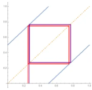
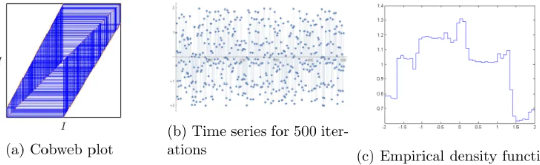
Figure 2.1: Plot of θ1 (blue line); γ(0.3) (red line) versus an orbit with initial condition
very close to 0.3 (purple line)
θ1(x) =
(
x+1/2 if 0≤x≤1/2
x−1/2 if 1/2< x≤1
Since the slope of θ1(x) is equal to 1, the graph of θ1 is parallel with respect to the line
y=x. It’s also expected orbits with periodic behavior. From the previous graphic, it’s easy to verify that orbit of x= 0.3 is a cycle of period 2. By choosing a x-point very close to
x= 0.3 we come up with a similar orbit (purple line).
Consequently, θ1(x) is stable because the distance between both orbits is bounded by a
scalarε >0. In this particular example εis equal to δ. Moreover,θ1(x) is not
asymptoti-cally stable since the distance between both orbits doesn’t converge to 0.
As opposed to stable, we now introduce the notion of unstable trajectories:
Definition 2.6. A trajectory τ(x) is called unstable or not stable if there is a ε > 0
such that, for all δ >0, there is ay ∈D such that |y−x|< δ but |θn(y)−θn(x)| ≥εfor
somen≥0.
In other words, no matter how close two trajectories start from each other, they will inevitable diverge.
The next theorem clarifies how we can categorize the different types of fixed points:
Theorem 2.2. Let θ be a function of class C1 andx be a fixed point of θ:
(i) If |θ′(x)|<1, then x isasymptotically stable
(ii) If |θ′(x)|>1, then x isunstable
Proof. See the Appendix - Section A.3 (page 35).
2.6.2 Expansivity
A map θ from an unstable system that satisfies the following theorem is named ex-pansive. A map whose pth iterate θp is expansive, but θ0, ..., θp−1 are not expansive, is
known asp-expansive.
Theorem 2.3. Let θ be differentiable almost everywhere on D and assume that there exists an integerm≥1 such that|(θm)′(x)| ≥δ >1, for all x∈D where the derivative is
defined, then all trajectories in (θ, D) are unstable.
2.7 Chaos: an Informal Perspective
Chaos theory is the study of nonlinear dynamics with unstable trajectories. Such dynamics seems surprisingly random and unpredictable.
There isn’t a single definition for chaos. Mathematicians diverge on the enough con-ditions to name a system as chaotic. Nevertheless, we’ll introduce chaos according to Devaney (1989) [8].
Remark 2.1. If a trajectory τ(x) is unstable in the sense of the Definition 2.6, then it has sensitivity to initial conditions.
For instance, if a map has sensitivity to initial conditions, then small errors could emerge in the attempt to compute numerically the map’s dynamic.
Definition 2.7. Let θ :D → D. θ is topologically transitive if for any pair of non-empty open setsU andV inD, there is a non-negative integerk such thatθk(U)∩V 6= 0.
Vaguely, a topologically transitive map has points which eventually move under iter-ation from one arbitrarily small open set to any other. Consequently, such a dynamical system cannot be decomposed into two disjoint open sets (Cattaneo et al (1997) [3]).
Convention 2.1. Denote bycl(A) the topological closureof A.
Definition 2.8. A is dense(or a dense set) in B if cl(A) contains B.
Definition 2.9. When θ(I) =I, then I is called an invariant set.
Finally we have all the proper mathematical tools to characterize a chaotic system.
Definition 2.10. (Devaney’s chaos)Let Dbe a set in Randθ:D→D. θ ischaotic onD if:
(i) θ is sensitive to initial conditions;
(ii) θ is topologically transitive;
(iii) periodic points are dense in D.
Example 2.6. (Logistic map)Let θ: [0,1]→[0,α/4]be θ(x) =αx(1−x). The map has
two fixed points: θ(x) = 0and θ(x) = α−α1 (their stability rely on α). Denavey (1989) [8] and Holmgren (1994) [10] states that family of logistic maps are chaotic ifα >2 +√5.
3
Statistical Dynamics
In the previous chapter we were focus on the qualitative properties of deterministic dynamical systems and their point-wise orbits/trajectories when n drives to ∞. Never-theless, in real life we are seldom capable to observe the precise states or the exact values of a system (θ, D). Statistics help us to approach this issue, recognizing that a statex+ε, where εis the observational error, has an intrinsic probability of happening. Such mea-sures are possible using random variableswhich are real-valued functions that gives a numerical quantity to any state ofD, i.e. X:D→R(later on we refer this function as an
observable). The purpose of this chapter is to develop statistical indicators for evaluate the asymptotic behavior of the random variables by exploiting all the possible information inside (θ, D).
Before starting this section, we need to recall some results from Measure Theory:
Definition 3.1. A σ-algebra is a collection of subsets F of a set D: (i) that contains D, i.e., D∈ F
(ii) that contains the complement of any set in F, i.e., A∈ F implies Ac∈ F
(iii) that contains the union of any countable collection of subsets inF, i.e., let{An}∞n=1
be a countable collection of sets with An∈ F for all n; then S∞n=0An∈ F
Definition 3.2. LetB(A)denotes the Borelσ-algebra onA. B(A)is the smallestσ-algebra that contains all the open sets ofA.
Definition 3.3. Let {An}∞n=0 be a countable collection of disjoint sets in a σ-algebra F.
A measure is a map µ:F →R+0 such that: (i) µ(∅) = 0
(ii) µ(S∞n=0An) =P∞n=1µ(An)
Definition 3.4. A measure space is a triple (D,F, µ) whose F is a σ-algebra of subsets ofD andµis a measure defined on F. The sets in F are called measurable. The measure space is called finite if µ(A) < ∞ for all A ∈ F. The measure µ is called a probability measure if µ(D) = 1 and therefore (D,F, µ) is a probability space.
Definition 3.5. Let (D,F) be a measurable set and (R,T) a topological set. A function
g:D→Ris said F-measurable if and only if the preimage of A underg belongs toF for all open setA∈R.
Definition 3.6. Let (D,F, µ) be a probability space and each random variable Xn is F
-mensurable for n≥0. A family of random variables {Xn}n≥0 is called a stochastic (or
random) process. Any stochastic process can be seen as a function of two variables: n
and ω. For each fixed n, ω → Xn(ω) is a random variable. On the other hand, if we fix
Definition 3.7. Given a probability space (D,F, µ), a F-mensurable system (θ, D) and an integrable observableX:D→R, we defineXn=X◦θn for alln≥0 as the stochastic
process which evaluates the states overγ(x), whereX=X0 is the initial condition and θn
the deterministic transformation at the instantn.
Definition 3.8. A stochastic process {Xn}n≥0 is stationary if the random vectors (X0,
X1, X2, ..., Xm) and (Xh, Xh+1, Xh+2, ..., Xh+m) have the same joint distribution for all
h, m≥0.
Definition 3.9. The support of a probability measure is the smallest closed set of full probability. We denote the support ofµ by supp(µ).
Example 3.1. Let (D,F) be a measurable space,x∈D and δ the Dirac measure defined as:
δx(A) =
(
1 x∈A
0 x /∈A
Sinceδx(D) = 1, the full probability set is {x}. Hence, the support of δx is also {x}.
Definition 3.10. Suppose (θ, D) isF-measurable. θ is calledmeasure preserving and
µis calledinvariant with respect toθif, for allA∈ Fθ =θ−1(B) :B∈ B , the
push-forward measure ofµtoθis exactly equal to the measureµ, i.e. θ∗µ=µ θ−1(A)=µ(A).
Remark 3.1. It’s easy to see that θ∗µ is a measure in the sense of the Definition 3.3.
Theorem 3.1. (Change of variable formula) Let θand ψbe F-measurable functions in R. ψ is integrable with respect to the push-forward measure θ∗µ if and only if the composition ψ◦θ is integrable with respect to the measure µ. Moreover the following formula holds:
Z
A
ψd(θ∗µ) =
Z
θ−1(A)
ψ◦θdµ
Proposition 3.1. If µ is an invariant measure to θ, then Xn=X◦θn is stationary.
Proof. See the Appendix - Section A.4 (page 36).
Remark 3.2. In particular, E(Xn) =E(X).
3.1 The Recurrence Theorem
LetPNn=0−1χA(θn(x)) be the number of times that the firstN iterates ofxwill visit the setA. The next theorem states that after wait enough time the orbit of x will eventually enter inA, but not once: it will enter infinitely times.
almost all points of A return to A infinitely often. That is, for almost x∈A:
lim N→∞
N
X
n=1
χA(θn(x)) =∞
Proof. See the Appendix - Section A.5 (page 37).
This theorem appeared in the statistical physics and it’s related to some of the most famous paradoxes in the mechanic physics field.
3.2 Limit Sets and Attractors
In the Chapter 2, stable periodic trajectories were introduced and their limit points are simply the elements of the periodic orbit to which trajectories converge (recall Definition 2.5). However, a general definition for limit set can emerge to consider chaotic systems.
Definition 3.11. The limit set ω(x) of the trajectory τ(x) is defined to be the set of all limit points of τ(x), i.e., ω(x) := T∞
n=1
cl[γ(θn(x))], where γ(y) is the orbit fromy.
Definition 3.12. An attractor for θ is a closed set L⊂D such that ω(x) =L for x in a setB of positive Lebesgue measure. The set B is called the basin of attraction of L.
Remark 3.3. Note that ω(x) is closed and θ(ω(x)) = ω(x). Obviously, L ⊂ B and
θ(L) =L.
3.3 Ergodic Dynamical Systems
Ergodicity relates the notion of recurrence introduced by Theorem 3.2 and the existence of invariant sets. A system is saidergodicif its trajectories enter in an unique invariant set without leaving it. In particular, that set cannot be decomposed in different parts with similar properties, which leads us to the next definition:
Definition 3.13. Let (D,F, µ) be a probability space. The dynamical system (θ, D) is
µ-ergodic if the measure of every undecomposable invariant set is either 0 or 1, i.e., if
A∈ F, then θ−1(A) =A implies either that µ(A) = 0 or that µ(A) = 1.
As a consequence, ergodic systems imply that time averageis equal to space aver-age. In general, this is not true, because the measureµcan take any value from 0 to 1. In this case,µcan only take the values 0 or 1, furthermore it’s also invariant to the system.
Theorem 3.3. (The Birkhoff-von Neuman Mean Ergodic Theorem)Let(D,F, µ)
be a probability space and letθbe a transformation which is measure preserving and ergodic. Let X be an integrable observable, then:
lim n→∞
1
n
n−1
X
i=0
Remark 3.4. In the conditions of the previous theorem, Xn = X ◦θn is an ergodic
process.
The left side of the equation from last theorem is the time average value of Xn and the right side is the space average ofXn defined explicitly as: µ(1D)RD(X◦θn)(x)dµ.
Corollary 3.1. Let (D,F, µ) be a probability space and let θ be measure preserving and ergodic on D. Then for µ-almost all x in D, τ(x) will visit every measurable set propor-tionally to its measure.
Proof. Let A ∈ F be a set with positive measure. If a trajectory τ(x) starts in D, how much time doesτ spend in A?
LetX =χA(x) =
(
1 if x∈A
0 if x /∈A defines if a pointx∈τ “enters” (or not) inA.
In general, (X◦θi)(x) =χA(θi(x)) =
(
1 if θi(x)∈A 0 if θi(x)∈/A
According to Theorem 3.2, the sum of all points in τ that enters in the set A will be infinite becauseA has positive measure. But by the Theorem 3.3 the average time spent in the setA can be determined by:
lim n→∞
1
n
n−1
X
i=0
χA θi(x)=
Z
D
χAdµ=
Z
A
dµ=µ(A)
3.4 Distributions for Dynamical Systems
3.4.1 Absolute Continuity: Density and Distribution
Now we’ll explore what kind of measures can be intimately related to distributions or density functions.
Convention 3.1. We denote the Lebesgue measure in R by λ.
Definition 3.14. A measure is said to be absolutely continuous with respect to λif for allA∈ F there exists an integrable functionf, called the density of µ, such that:
µ(A) :=
Z
A
f(x)dx=
Z
θ−1(A)
f(x)dx=θ∗µ(A)
Remark 3.5. Ifµis absolutely continuous the Theorem 3.1 is equivalent to the Definition 3.14.
Such measures are differentiable in the sense of the Radon-Nikodym derivative
Rb
af(x)dx. Note that under these conditions f is unique as well as continuous λ-almost everywhere.
Definition 3.15. Let µ1 and µ2 be two measures on the same measure space (D,F). We
sayµ1 is absolutely continuous with respect toµ2 or µ1<< µ2 if for any set A∈D, such
thatµ2(A) = 0 always implies µ1(A) = 0.
Definition 3.16. Let f : D → R be a density function and D a subset of R. The set-theoretic support of f is the closure set of points in Dwhere f is non-zero, i.e.:
supp(f) =cl({x∈D|f(x)6= 0})
Convention 3.2. Acipis the abbreviation for absolutely continuous invariant probability measure and its density is calledinvariant density.
Remark 3.6. If µ is an acip, thensupp(µ) is equal to supp(f).
Example 3.2. Recall the map from Example 2.3 where s= 2:
θ2(x) =
(
2(x−1/2) + 1 if 0≤x≤1/2
2(x−1/2) if 1/2< x≤1 =
(
2x if 0≤x≤1/2
2x−1 if 1/2< x≤1
Let f =χ[0,1], where f is the density function of Lebesgue measure restricted to [0,1]. We’ll use the results from Theorem 3.1 and Definition 3.14 to show thatµ is an acip:
θ∗µ([a, x]) =
Z
θ−1([a,x])
χ[0,1]dλ=
Z
[a,x] 2
1dλ+
Z
[a,x] 2 +
1 2
1dλ=x−a=
Z
[a,x]
χ[0,1]dλ=µ([a, x])
Definition 3.17. (Strongly ergodic dynamical systems)A dynamical system (θ, D)
that is ergodic with respect to an absolutely continuous measure µ defined on R will be called strongly ergodic. For a strongly ergodic system with density f, the measure is equivalent to the cumulative distribution function:
F(x) :=µ([a, b]) =
Z x a
f(u)du=
Z x
infD
f(u)du
If we extend θtoRin the usual way, then we obtain F(x) =R−∞x f(u)du.
Theorem 3.4. (Lasota-Yorke, 1973) Let θ :D→ D be a piecewise function of class
C2 where Dis an interval. If |θ′(x)| ≥δ >1 λ-almost everywhere inD, then there exists
an acip forθ.
Example 3.3. This result applies to piecewise linear systems like the system presented on
(2.1c)with βi >1.
3.4.2 The Number of Absolutely Continuous Invariant Ergodic Measures
The next theorem sets up sufficient conditions to establish a maximum number of ergodic acips in D. In addition, it tells us what we should expect for the shape of their supports. The extension of the following work is available on Section 8.2 from Boyarsky & G´ora (1997) [1].
Theorem 3.5. Let (θ, D) be a dynamical system whereDis an interval and the mapθ is piecewise withddiscontinuity points and strictly monotonic on each piece of the partition
D of interval pieces Di, i = 1, ..., d+ 1. Assume that for each i = 1, ..., d+ 1, θ is
restricted to the interior of Di and it is continuously differentiable and expansive. Then
there exists at mostd (could be less) ergodic acipsµi whose supports are union of finitely
many intervals.
As an immediate consequence of Theorem 3.5 and Definition 3.12 we get:
Corollary 3.3. There exists a partition {Bi, i= 1, ..., m} of D such thatBi is a basin of
attraction ofsupp(µi). Moreoversupp(µi) is an attractor forθ and this implies at most d
attractors.
Remark 3.7. If the map has only one discontinuity point (d= 1), then there exists an unique ergodic acip with an unique attractor that is the union of closed intervals.
3.4.3 The Mean and Variance of a Trajectory
Let {Bi, i= 1, ..., m} be the partition imposed by Corollary 3.3. From Theorems 3.3 and 3.5 we have:
Corollary 3.4. Let fi= dµdλi for each ergodic acipµi. Then for all x∈Bi,
lim n→∞
1
n
n−1
X
k=0
X◦θk(x) =
Z
D
X(u)fi(u)du
In particular, for allx∈Bi, the expected or mean value of states in the trajectory is:
¯
µi = lim n→∞
1
n
n−1
X
k=0
θk(x) =
Z
D
ufi(u)du
and the variance of states in the trajectory is:
¯
σi2 = lim n→∞
1
n
n−1
X
k=0
h
θk(x)−µ¯i2=
Z
D
(u−µ¯)2fi(u)du
3.5 Constructing Densities
3.5.1 The Frobenius-Perron Operator
Let (θ, D) be a dynamical system, where D is a finite interval [a, b] and suppose that
µis an ergodic acip with an invariant density f.
Definition 3.18. The Frobenius-Perron Operator is defined by:
P f(x) = d
dx
Z
θ−1([a,x])
fdλ
Proposition 3.2. (Properties of P)
(i) P :L1 → L1 is linear, where L1 is the space of integrable functions.
(ii) P f ≥0 if f ≥0
(iii) R P fdλ=R fdλ
(iv) P f =f if and only if µ(A) =RAfdλfor all A is invariant under θ
Proof. See the Appendix - Section A.6 (page 38).
3.5.2 The Frobenius-Perron Operator for Piecewise Monotonic Systems
Now, we will show how the P f operator can be used for piecewise monotonic maps.
Proposition 3.3. Let θ be a piecewise, strictly monotonic map satisfying Theorem 3.4. Let Li be an attractor which is the support of an ergodic acip µi. Then µi has an unique
invariant density function f(x) that satisfies:
P f(x) = n
X
i=1
f(θi−1(x))·
dθi−1(x)
dx
·χ[θ(ai−1),θ(ai)](x)
Proof. It comes from simple calculations and basic Lebesgue integration rules. For the complete proof see Section 4.3, page 85 and 86 from Boyarsky & G´ora (1997) [1].
3.5.3 Empirical Approach to Density Functions
Despite the fact that Frobenius-Perron operator offers a more precise formula for the density function f, in most cases we are not able to compute it analytically due to the complexity of the map. Instead, we may approachfnumerically by collecting experimental data. Recall Definition 3.17 for the cumulative distribution function (denoted by F). Let
Xbe a random variable, then: F(z) = Prob[X≤z] =R−∞z f(x)dx,wheref is the density function ofX. See more in Evans et al (2011) [9].
toµ((−∞, z]). Since µ is an absolutely continuous measure with respect to λ, we have:
µ((−∞, z]) = F(z). This result allows us to use the time average to build our empirical distribution.
Lemma 3.1. Theempirical cumulative distribution functionfor a random variable
X is denoted by ecdf and it has the following expression:
ecdf(z) =µ((−∞, z]) = 1
n
l−1
X
i=0
χ(−∞,z]◦θi(x),
wherendetermines how many elements are insideτ(x) andlis the number of points used to build the empirical cumulative distribution function.
In principle, ecdf should be a function of z and x. However, by the ergodic theorem ecdf(z, x) is equal to ecdf(z) for µ-almost every x. This means that from a probabilistic point of view we can remove the dependence onx.
The use of empirical data should lead to a cumulative distribution function quite similar to the real underlying distribution. However, we don’t have the same ease for the density function. In order to get a fair replicate of the true density function f, we need a large amount of data. Otherwise, for close values ofz the cumulative distribution function has similar values and therefore the density function near those points goes (wrongly) to 0. Plus, the functionχ is not smooth because it isn’t differentiable everywhere. This is why in the expression of ecdf we need to declare a variablel distinct of n. Note that with a largel, on the one hand, we have more points to draw our ecdf, but the density function will require lots of data to distinguish consecutive points. Hence, choosing a small but not too smallland a largen(inducing some sort of smoothness) we can simulatef numerically and see some resemblances to the true density function.
Lemma 3.2. The invariant density function f may be numerically obtained by:
f(z1)≈
ecdf(z2)−ecdf(z1)
δ , z2 > z1, δ=
1
l−1
Example 3.4. See the complete example in the Appendix - Section A.7 (page 39).
Remark 3.8. The code used to compute the empirical distribution in the previous example is available in the Appendix - Section A.8 (page 41).
3.6 Other Statistical Properties
Despite the “sensation” of randomness intrinsic to chaotic dynamical systems, they are not actually stochastic processes because for an initial conditionxn, the value for the next iterationxn+1 is exactly known by a deterministic map. However, this kind of trajectories
to be a realization of a stochastic process (generating a series of independent, identically distributed random variables). Now we’ll see how the ergodic theory can be related (in a certain way) to a few important results in Probability Theory.
Theorem 3.6. (Strong Law of large number) Recall the definition of the stochastic process{Xn}n≥0, where allXn=X◦θnrepresent a sequence of independent and identically
distributed random variables. Then, by the strong law of large numbers, the sample average (time average) converges with probability 1 to the expected value E(X) (space average):
µ lim n→∞
1
n
n−1
X
k=0
Xk=E(X)
!
= 1, µ-almost surely
Proof. It’s an immediate consequence of the ergodic theorem (see Theorem 3.3).
Note that the values of trajectories are not random and not necessarily independent among them. Therefore the Theorem 3.3 must be seen as a generalization of the law of large numbers.
From now on, let (θ, D) be in the conditions of Theorem 3.5 and suppose d= 1. By Remark 3.7 there exists only one acipµ. In addition, suppose that (θ, D) is topological mixing, i.e.:
Definition 3.19. Let θ:D→ D be a real-valued function. θ is topological mixing if for all intervalI subset of D there is a non-negative N such that θN(I) =D.
In order to evaluate how fast the observableXn=X◦θn becomes independent of the initialX0 =X, Boyarsky & G´ora (1997) [1] established the following result:
Theorem 3.7. (Decay of correlations) For any bounded observable X :D → R and
m≥0, we have:
ρ(Xm, Xn) = lim
n→∞|E(Xm, Xn)−E(Xm)E(Xn)|= 0
Proof. See Definition 8.3.1 and Theorem 8.3.2, page 148 from Boyarsky & G´ora (1997) [1].
When time average and space average are similar3, the sum of the observations under the processXn converges in limit to a standard normal distributionN(0,1).
Theorem 3.8. (Central Limit Theorem) For any bounded observable X : D → R, there is aσ >0 such that:
lim n→∞µ
"
1 σ/√n
n−1
X
i=0
Xi−nE(X0)
!
< z
#
= √1
2π
Z z
−∞ exp
−x 2
2
dx
Proof. See Theorem 8.5.1, page 157 from Boyarsky & G´ora (1997) [1].
3If ngoes to
∞, the quotient 1
σ/√n goes equally to
∞; then, the limit is only bounded byz when the
4
Dynamics of Lorenz Maps
Before diving in the discussion of the market model of Tramontana et al (2010) [18], we need to declare some results regarding the class of maps present in their work. The next definition comes from Hubbard & Sparrow (1990) [13]:
Definition 4.1. Let θ: [0,1]→[0,1] be a function of class C1 satisfying:
(i) There is a d∈(0,1) such that θ is continuous and strictly increasing on [0, d) and on (d,1];
(ii) limx→d−θ(x) = 1 andlimx→d+θ(x) = 0;
(iii) θ is (topologically) expansive;
thenθ is a Lorenz map.
Letθs take the form of the map from Example 2.3:
θs(x) =
(
s(x−1/2) + 1 if 0≤x≤1/2
s(x−1/2) if 1/2< x≤1 (4.1)
θsis a particular form of a Lorenz map called symmetric piecewise linear Lorenz
map because it is a symmetric function on the discontinuityd=1/2. Moreover, θs is an
odd function4.
Lemma 4.1. Let ϕ(x) = 1−x, then θs isϕ−symmetric, i.e.: θs◦ϕ=ϕ◦θs.
Theorem 4.1. Let θs be a symmetric piecewise linear Lorenz map. θs has an unique
ergodic acipµ. Moreover, this measure is ϕ-symmetric, i.e. ϕ∗µ=µ.
Proof. From the Theorem 3.5, θs is a class C1 expansive and a continuous function on the partitions D1 and D2. By the first condition of the theorem we have d = 1. Then
it follows µi is equal to µ1. Therefore, µ1 is the unique admissible acip. With the result
from Remark 3.7, the proof is straightforward.
Remark 4.1. We say that an interval I is ϕ-symmetric if ϕ(I) = I, which means the interval I is symmetric with respect to x=1/2.
Lemma 4.2. Suppose s ∈ 1,√2. Let J = 1− 1 2s,12s
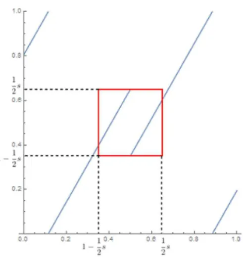
be ϕ-symmetric and hs :J → [0,1]the affine transformation hs(x) = s−11 x+12s−1, then hs◦θs2◦h−s1=θs2 holds.
Proof. First we need to calculate an explicit expression for θ2s. Due to the fact θs is a piecewise function the composition θ2
s = θs ◦θs won’t be a straight forward expression.
θs has a discontinuity at x = 1/2, so we will expect that θ2s also has a discontinuity at
4A function θis odd ifθ(x) +θ(
Figure 4.1: Graph ofθ2
s with s= 1.3 (blue line) and the setJ (red box)
θs(x) =1/2and two other discontinuity points. After some calculus, we come up with this
expression (whereu= 12 −21s):
θs2(x) =s2(x−1/2) +
1
2s+ 1 if 0≤x≤u
1
2s if u < x≤1/2 −12s+ 1 if 1/2< x≤1−u −12s if 1−u < x≤1
The Figure 4.1 shows when θs2 is restricted to J, there is a striking resemblance to the plot ofθs. In some sense, the function inside of the red box may be understood as a smaller version ofθ with a slope equals tos2.
The inverse function of hs has the following expression:
h−s1(x) = (s−1)x−1
2s+ 1
Now, we’ll get the expression hs◦θ2s◦hs−1 step-by-step. First compute θs2◦h−s1:
s2
(s−1)x−1
2s+ 1−1/2
+
1
2s+ 1 if 0≤h−s1(x)≤u
1
2s if u < h−s1(x)≤1/2
−21s+ 1 if 1/2< hs−1(x)≤1−u
−1
2s if 1−u < h−s1(x)≤1
Whereash−1
s : [0,1]→J, the range ofhs−1 is only defined onJ ⊂[0,1]. Plus, by visual proof we already know from the plot ofθ2s thatu <1−1
2s(the complete proof is obtained
branches because they don’t lie onJ. Then, we replaceu by a stricter condition 1−1 2s.
θs2◦h−s1(x) =s2
(s−1)x−1
2s+1/2
+
(
1
2s if 1−12s≤hs−1(x)≤1/2
−21s+ 1 if 1/2< hs−1(x)≤ 12s
Finally,
hs◦θs2◦h−s1
(x) =
(
s2(x−1/2) + 1 if 0≤x≤1/2
s2(x−1/2) if 1/2< x≤1 =θs2(x)
Intuitively the previous lemma states the existence of a suitable affine function hs which allows us to transform the information provided byθ2
s in a smaller scale,θs2. Thus,
θs2 and θs are somehow related. The goal of the next results is to deepen that relation under the setJ.
Remark 4.2. Note that if J =1−1 2s,12s
is ϕ-symmetric and invariant, then the fol-lowing inequality must hold:
1−1 2s <−
1 2 s
3−s2−s
Lemma 4.3. Suppose s ∈ (√2,2], then θs is topological mixing, i.e. for all I subset of [0,1], there is a n∈Nsuch that θns(I) = [0,1].
Proof. See the Appendix - Section A.9 (page 42).
Corollary 4.1. Ifs∈ √2,2andf is the ergodic invariant density ofθs, thensupp(f) = [0,1]and the attractor is also [0,1].
Proof. This follows from the fact thatsupp(f) is invariant and contains an interval I. By iterating this interval and due to the previous lemma we getsupp(f) = [0,1].
Definition 4.2. Ifθ is topological mixing, then θis called prime (in the sense that is not divisible).
Lemma 4.4. Let θ1 : D1 → D1 and θ2 : D2 → D2 be two arbitrary functions and
D2 ⊂D1. Suppose there exists a bijective function h such that θ2◦h = h◦θ1. Then θ1
is prime if and only if θ2 is also prime (the property of being prime is invariant under
conjugacy).
Proof. By the lemma’s hypothesis, for any subset ofD1, sayI, we haveθn1(I) =D1. If we
choose an intervalJ as a subset ofD2, then there exists an >0 such that (θ1n◦h−1)(J) =
If we take the nth iterated of θ2(J) we come up with: θn2(J) = (h◦θ1 ◦h−1)n(J) =
(h◦θ1n◦h−1)(J) =h(D
1) =D2.
Definition 4.3. We call the order of renormalization of θs the number:
n= maxnk≥0 :s2k ≤2o,
and we sayθs isn-times renormalizable.
Directly from the previous definition,θs isn-times renormalizable if the valueslies in the interval 22n1+1,221n
i
. Nonetheless θs is prime and also 0-times renormalizable when
sbelongs to √2,2. In the latter case we may also sayθs is not renormalizable (n= 0). Furthermore the setJ, introduced on Lemma 4.2, depends on the order of renormalization
nand we will henceforth denote it asJn.
Example 4.1. Suppose θs is 2-times renormalizable, that is s∈
218,2 1 4
i
. Then:
(
hs◦θs2◦h−s1=θs2
hs2 ◦θ2
s2 ◦h−s21 =θs4
, (4.2)
where hs is the function introduced by the Lemma 4.2.
The goal is to find a bijective function which relatesθ4s with θs4 restricted to a certain
set, sayJ2. Rewriting the expression of θs22 as the composition θs2 ◦θs2:
θs22 =θs2 ◦θs2 = hs◦θ2s◦h−s1◦ hs◦θ2s◦h−s1=hs◦θ4s◦h−s1
Now we’ll use this result to replace in the second equation of (4.2):
θs4 =hs2 ◦θs22 ◦h−s21=hs2 ◦hs◦θ4s◦h−s1◦h−1
s2 = (hs2 ◦hs)◦θs4◦(hs2 ◦hs)−1
The bijective function we are looking for is defined ashs2◦hs. Therefore this function
is our conjugation:
J2 J2
[0,1] [0,1] θ4
s
hs2◦hs hs2◦hs
θs4
whereJ2 = (hs2 ◦hs)−1([0,1]). Note thats4 ∈(√2,2]. Henceθs4 : [0,1]→[0,1]is prime,
thenθ4s restricted to J2 is prime.
Lemma 4.5. Let θs ben-times renormalizable. Moreover, letgn=hs2(n−1)◦ · · · ◦hs2◦hs,
then the mapθ2sn :Jn→Jn, where Jn=
h
s2(n−1)◦ · · · ◦hs2 ◦hs
−1
([0,1]), is conjugated toθs2n : [0,1]→[0,1] through gn, i.e.:
Jn Jn
[0,1] [0,1] θ2n
s
gn gn
θs2n
From the previous lemma and by the fact that θ2sn restricted to Jn is prime, the following corollary arises:
Corollary 4.2. If s∈22n1+1,221n
i
, then the support of the ergodic acip is the union of
Jn, θs(Jn±), ..., θ2
n−1
s (Jn±), where Jn−=Jn∩
0,12 and Jn+=Jn∩
1
2,1
.
Remark 4.3. By the previous corollary, thesupp(f) is an union of 2n+1−1 intervals.
Figure 4.2: The graph explains for an initial condition onJnhow the path of the trajectory is
Proposition 4.1. The set Jn has the following neat representation:
Jn= [an, bn], where an= n−1
X
i=0
1−s 2i
2
!
i−1
Y
j=0
s2j−1
, bn=
n−1
Y
i=0
s2i−1
!
+an
Proof. See the Appendix - Section A.10 (page 42).
Corollary 4.3. The length of interval Jn tends to zero when s drives to 1.
Proof. If we assumesgoes to 1, by the Definition 4.3 the order of renormalization nwill never be upper bounded. Hencengoes to∞ and then we have:
lim
s→1|bn−an|=
∞
Y
i=0
s2i−1= 0,
5
Applications: a Simple Financial Market Model
The model proposed by Tramontana, Westerhoff and Gardini is a combination of several papers and contributes from the literature of agent-based financial market models. According to their formulation, the interactions between heterogeneous agents, bounded by simple technical and fundamentalist trading rules, may generate very interesting and complex price dynamics, containing the appearance of financial distress events such as bubbles and crashes. This model is closely related to the models found on Day and Huang (1990) [6] and Huang and Day (1993) [12].
A survey study presented by Menkhoff & Taylor (2006) [16] proves market specula-tors believe in technical and fundamental analysis to forecast prices on financial markets. Fundamentalists support their trading strategies on the idea the price of an asset will eventually revert to its (estimate) fundamental value (constant value known to all market contestants) and stays there for awhile. In the bear (undervalued) market, when the mar-ket prices are smaller than their fundamental value, fundamentalists seek for investment opportunities as buyers and the lower the price, more aggressive fundamentalists are. Due to their conventional approach, they usually contribute to the stability of the market. On the other hand, chartists, technical analysts or just noise traders disregard the hypothesis of the prices revert to their fundamental value. Instead, they evaluate the future prices of the market based on the chart analysis, which consists studying historical price pat-terns and exploit them to make (destabilizing) investment decisions. Chartists are more comfortable to explore investment opportunities as buyers in the bull (overvalued) mar-ket because they believe the prices will continue rising. Fundamentalists and chartists may responds with asymmetrically aggressiveness, different trading horizons/volume and market entry levels whether they are facing a bull or bear market. Thus, the model dis-tinguishes fundamentalists or chartists in two types. Type 1 speculators are always active in the market regardless the price. Type 2 speculators are more conservative and they are only able to interact in the market if the mispricing (absolute difference between the asset price and its fundamental) reaches to a certain critical value. Type 2 fundamentalists believe the investment opportunities close to the fundamental value are worthless due to the slim chances to be profitable. Type 2 chartists don’t trust the persistence of bull or bear markets when the mispricing is close enough to the fundamental value.
In order to reduce the positive or negative excess of demand, the market maker adjusts the prices to reach a classic market equilibrium (in the sense of the basic hypotheses of the law of supply and demand). Therefore, the market maker quotes the market prices under the following rule: Pn+1 =Pn+a
DnC,1+DC,n2+DF,n1+DF,n2
, whereP is the log price,
Surprisingly, this whole financial plot can be represented as an one-dimensional dis-continuous piecewise-linear system. Depending on the form ofDnC,1, DnC,2, DnF,1 and DnF,2, the system may (or not) have chaotic dynamic (led by unstable orbits) and multiple dis-continuity points. Further in this chapter, we will demonstrate even with such a simple mathematical setup the possibility to generate very interesting dynamics (which allows us to study the bull-bear market phenomena). In this way, this deterministic model is already capable to incorporate some stylized facts from financial markets like bubbles, crashes and excess of volatility. In the next section we are disclosure one possible shape forPn+1.
5.1 Setup with One Discontinuity Point
The one discontinuity model is presented according to Tramontana et al (2010) [18].
Type 1 chartistsbelieve in the persistence of bull (+) and bear markets (−), then their orders are specified as:
DC,n1 =
(
c−1(Pn−F) if Pn−F <0
c+1(Pn−F) if Pn−F ≥0
, (5.1)
wherec+1 and c−1 are positive reaction factors and F is the log of the fundamental value. This type of speculator will take buying (selling) positions if the prices are above (bellow) the fundamental value. If c+1 > c−1, the chartists are trading more aggressive in the bull market than the bear market. On the other hand, the chartists are submitting orders with larger size in the bear market ifc+1 < c−1.
Type 2 chartistssubmit their orders based on the following rule:
DC,n2 =
−c−2 if Pn−F <0 0 if Pn−F = 0
c+2 if Pn−F >0
, (5.2)
where c+2 and c−2 are positive reaction factors. This type of chartists still believe in the persistence of bull-bear markets but they assume an idle position when the price is equal to its fundamental value. The size of the orders are now only subordinate to the reaction factorsc+2 (order size in the bull market) andc−2 (order size in the bear market), no matter how far or close the price is to the fundamental value.
On the contrary, type 1 fundamentalists believe the prices will converge to their fundamental value in the long run, then their orders are placed according to:
DF,n1 =
(
−u−1(Pn−F) if Pn−F <0
−u+1(Pn−F) if Pn−F ≥0
, (5.3)
fundamentalists take buying (selling) positions in the bear (bull) market hopping the price will eventually rise up (fall) to the fundamental value. Moreover, type 1 fundamentalists may respond asymmetrically to the bull and bear markets: whenu−1 > u+1 fundamentalists are more aggressive in the bear market andu−1 < u+1 otherwise.
Lastly,type 2 fundamentalistssubmit their orders under the following rule:
DF,n2 =
u−2 if Pn−F <0 0 if Pn−F = 0
−u+2 if Pn−F >0
, (5.4)
whereu+2 andu−2 are positive reaction factors. Type 2 fundamentalists are in an idle state when the price is equal to the fundamental value. Otherwise, they are buying (selling) orders by the size ofu−2 (u+2).
After a few variable changes, we come up with the following dynamical system which expresses the model in terms of the deviations from the fundamental value:
xn+1=ψ(xn) =
ψL(xn) =sLxn+mL if xn<0
ψC(xn) = 0 if xn= 0
ψR(xn) =sRxn+mR if xn>0
, (5.5)
wherexn=Pn−F,sL= 1 +c−1 −u−1,sR= 1 +c+1 −u+1,mL=u−2 −c2−andmR=c+2 −u+2. This map formulation is generally an one-dimensional discontinuous map, except for the very particular case when we omit type 2 speculators (mR = 0 and mL = 0) which has limited interest for our applications. Note thatsL,sR,mLandmRare linear combinations of positive factors, hence they can take any value inR. To simplify the work in the next sections and without loss of generality, let the mathematical model in (5.5) be reduced to5:
xn+1=ψ(xn) =
(
ψL(xn) =sLxn+mL if xn<0
ψR(xn) =sRxn+mR if xn≥0
(5.6)
As we explained in the Chapter 3, there are many cases where it’s very hard to ob-serve the states under their natural form. For instance, in a financial market, how many speculators can predict the exact asset’s closing price? Probably none. Without access to the real prices, how they decide to issue their orders? Some of them are able to get fair forecasts: instead of predict the exact prices, they perform prognoses based on price intervals by assuming an observational error6, say ε. That’s exactly the approach we are seeking. We assume an initial condition X which is an observable such that the states inD are assigned to a real number. Later we use the deterministic transformation of ψ,
5From the statistical standpoint, the branchψ
C is irrelevant because the probability of reachingx= 0
is zero.
6The price prediction is often associated with an observational error, the difference between the real
which is ourlaw of the market, to iterate X. This process is a particular application of the stochastic processXn already introduced in the Definition 3.7.
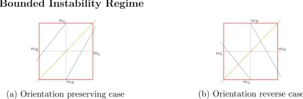
5.2 Bounded Instability Regime
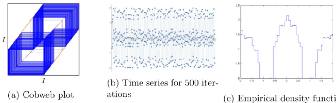
(a) Orientation preserving case (b) Orientation reverse case
Figure 5.1: Plot of two versions ofψpresented in this section (blue line) and the invariant intervalI (red box);y =x line (yellow line)
Different agent behavior and market price fluctuations are derived by manipulating the reaction factors. For the purposes of the thesis, we’ll restrict the model variables such that we get two distinct cases:
❼ For theorientation preserving case(see Figure 5.1a), type 1 chartists trade more aggressively in the bull/bear market than type 1 fundamentalists. This means the slopes sL and sR must be positive and greater than 1. On the other hand, for type 2 speculators, the fundamentalists trade more aggressively in the bull/bear market than chartists. This statement implies that mL is positive (intercept of the left branch) and mR is negative (intercept of the right branch). Inside the bull or bear market, when the current price increases (decreases), the future price increases (decreases).
❼ The orientation reverse case(see Figure 5.1b) may be seen as a negation of the previous case. For the type 1 speculators, fundamentalists are now trading more aggressively than chartists, therefore we assume that both slopes sL and sR are negative and less than−1. Simultaneously, type 2 chartists are trading more heavily than fundamentalists which suggestsmLis negative andmRis positive. In this case, whenever the current price inside the bull or bear market increases (decreases), the future price decreases (increases).
Since the slopes for both cases are greater than 1 in absolute value,ψ is an expansive map and so we expect its orbits be unstable. In these scenarios, which will be henceforth referred as the instability regime, only chaotic dynamics can occur.
Remark 5.1. The methods studied for the orientation preserving case can be applied to the orientation reverse case. Note that the second iteration for both cases (ψ2) is the same
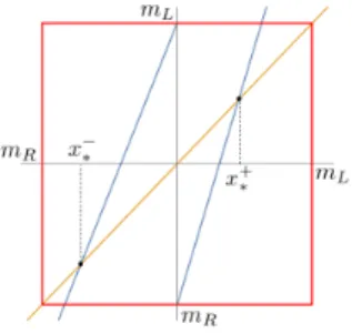
Therefore, we will only keep studying the orientation preserving case. Considering all the restrictions, two unstable fixed points can be determined: x−
∗ = 1m−LsL < 0 and x+∗ = mR
1−sR > 0. Any initial condition outside the interval (x
−
∗, x+∗) drives the orbit to
∞. From an economic point of view, the explosion of the dynamic gives practically no information regarding the evolution of the price because in the real markets prices won’t indefinitely rise or fall. Thus, we need to find more restrictive conditions to determine when bounded behavior is indeed a reality.
Lemma 5.1. ψhas bounded orbits if any initial condition lies on(x−
∗, x+∗)andmRbelongs
to the interval mL
1−sL, mL(1−sR)
or, alternatively, mL lies on
mR(1−sL),1m−RsR
. There is also an invariant interval I = [mR, mL] which absorbs the dynamic and don’t
never let it exit from I.
Proof. If any initial condition belongs to the interval (−∞, x−
∗)∪(x+∗,∞), the orbit ofxnis divergent towards∞. In addition, we know there exists an intervalI = [mR, mL] such that it’s an invariant absorbing interval. In that case the following conditions must hold: x−
∗ <
mR and x+∗ > mL. Then, we obtain the desire condition for mR =
mL
1−sL, mL(1−sR)
(or formL) by replacingx−∗ and x+∗ for their respective expressions.
Figure 5.2: Plot of ψ(blue line) where I (red box) is not an invariant interval
Otherwise, once the orbit of xn is inside I, it could escape from I. Figure 5.2 allows us to see what happen when the fixed points are insideI. There are two intervals which don’t verify the condition of invariance and they are [mR, x−∗] and [x+∗, mL].