Nonautonomous Di ﬀerence Equations with Applications

(1)

Nonautonomous Di

ff

_{erence Equations}

with Applications

Rafael Domingos Garanito Lu´ıs

(2)

(3)

(4)

(5)

Acknowledgments

My acknowledgments goes to my supervisors, Henrique Oliveira and Saber Elaydi, who en-couraged me and helped me in all the research problems. In addition, a special thanks goes to

Saber Elaydi due its efforts in improving my American English.

I also want to acknowledge the “Centro de Análise Matemática, Geometria e Sistemas Dinâmicos” and its chair Professor Carlos Rocha, who supported some of my trips to “Insti-tuto Superior Técnico”, to conferences and to Trinity University. A special thanks goes to the Department of Mathematics, of Trinity University and their members for its hospitality during my visits.

A special thanks to the “Fundação para a Ciência e a Tecnologia (FCT)” for the financial

support provided through the PhD grant SFRH/BD/40924/2007 financed by national funds

from Minist´erio da Ciˆencia, Tecnologia e Ensino Superior (MCTES).

Finally, this work was not possible without the “Licença para Equiparação a Bolseiro” from the “Secretaria Regional de Educação e Cultura - Governo Regional da Madeira” .

(6)

(7)

Resumo

Esta dissertação está dividida em duas partes. Na primeira parte apresentamos alguns con-ceitos e noções básicas que levam à construção de sistemas dinâmicos não autónomos discre-tos. Utiliza-se o conceito de “skew-product” para estudar algumas propriedades destes sistemas

no que concerne à sua periodicidade e estabilidade. É feita uma breve abordagem à variedade

central e à bifurcação dos pontos periódicos nas equações de diferenças não-autónomas unidi-mensionais.

Na segunda parte faz-se um estudo de alguns modelos aplicados `a ecologia/biologia e `a

economia. Devido à dificuldade em manipular certas relações que surgem no estudo que se faz aos modelos, apresentamos cálculo computacional por forma a ilustrar e a descrever a dinâmica do modelo.

Uma das principais contribuições desta tese é o estudo da estabilidade dos sistemas não-lineares quando o valor próprio se encontra no c´ırculo unitário. Outra é o estudo das bifurcações, em particular, o diagrama de bifurcação no espaço dos parâmetros, do modelo de competição entre duas espécies definido por equações de Ricker.

Constatou-se que a dinâmica do modelo de competição de Ricker é semelhante à do mod-elo log´ıstico de competição. Assim, acreditamos que deve existir uma certa classe de mapas bidimensionais para os quais se poderá generalizar os nossos resultados.

Finalmente, não podemos deixar de realçar as técnicas que se utiliza na prova da existência de solução positiva do sistema não-autónomo bidimensional de Ricker .

Key Words

Sistemas não-autónomos periódicos, Periodicidade, Estabilidade, Bifurcação, Modelos de competição, Efeito Allee.

(8)

(9)

Abstract

This work is divided in two parts. In the first part we develop the theory of discrete nonau-tonomous dynamical systems. In particular, we investigate skew-product dynamical system, periodicity, stability, center manifold, and bifurcation.

In the second part we present some concrete models that are used in ecology/biology and

economics. In addition to developing the mathematical theory of these models, we use simula-tions to construct graphs that illustrate and describe the dynamics of the models.

One of the main contributions of this dissertation is the study of the stability of some con-crete nonlinear maps using the center manifold theory. Moreover, the second contribution is the study of bifurcation, and in particular the construction of bifurcation diagrams in the parameter space of the autonomous Ricker competition model.

Since the dynamics of the Ricker competition model is similar to the logistic competition model, we believe that there exists a certain class of two-dimensional maps with which we can generalize our results.

Finally, using the Brouwer’s fixed point theorem and the construction of a compact invariant and convex subset of the space, we present a proof of the existence of a positive periodic solution of the nonautonomous Ricker competition model.

Key Words

Nonautonomous periodic systems, Periodicity, Stability, Bifurcation, Competition Models, Allee effect.

(10)

(11)

List of Tables

1.1 Types of bifurcation of nonhyperbolic fixed points in one-dimensional autonomous

maps . . . 22

1.2 Bifurcation conditions for nonhyperbolic periodic points in nonautonomous

one-dimensional maps. . . 40

(14)

(15)

List of Figures

1.1 A 2₋periodic geometric cycle on X = R2

+ and a 4−periodic complete cycle on

the skew productX_×YwhereY =_{F0,F1,F2,F3},Fi =(fi,gi),i=0,1,2,3 for

the difference equation defined in example 5. . . 10

1.2 A 6₋periodic cycle in a 9₋periodic system. . . 12

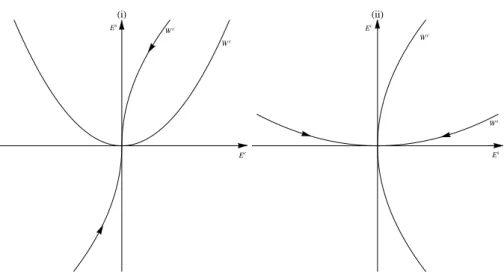
1.3 Stable and center manifold. In (i) we have σ(A) = σc andσ(B) = σswhile in

(ii) we haveσ(A)= σsandσ(B)= σc. . . 19

1.4 Stable and unstable manifold. . . 21

1.5 The bifurcation curves of a 2₋periodic cycle, in the parameter space, of the

2₋periodic Ricker equation. . . 32

1.6 The bifurcation surface where occurs the pitchfork bifurcation of the zero fixed

point of the equation xn+1 = fn(xn) where fn(x)=µnx−x3,µn> 0 and fn= fn+3

for alln= 0,1,2, . . .. . . 35

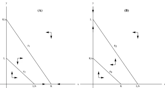
2.1 The stability of the exclusion fixed point and the validity of the competition

exclusion principle. (A) If 0 < K _≤ 2 and L < bK, then (K,0) is locally

asymptotically stable and speciesygoes extinct. (B) If 0< L_≤ 2 andL> K/a,

then (0,L) is locally asymptotically stable and speciesxgoes extinct. . . 43

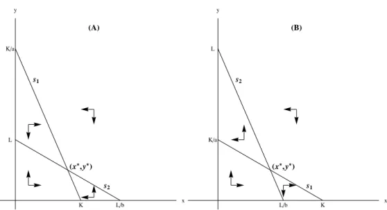
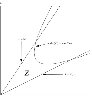
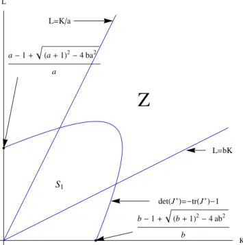
2.2 Isoclines: (A) The coexistence fixed point of Eq. (2.1) exists ifbK < L < K/a andab < 1. (B) The coexistence fixed point of Eq. (2.1) exists if K_a < L< bK andab>1. In this scenario this equilibrium is a saddle. . . 44 2.3 The relative position of the hyperbolasdet(J∗) = 1 and det(J∗) = ₋tr(J∗)₋1

and the linesL= bK andL= K/awhena= b= 1/2. The black curves are the

implicit solutions ofdet(J∗₎₌_{1 while the grey curves are the implicit solutions}

ofdet(J∗)= ₋tr(J∗)₋1. The stability regionS1 is enclosed by the two lies and

the left branch of hyperboladet(J∗)=₋tr(J∗)₋1. . . 48

2.4 The stability regions in the parameter space of the solution of the Ricker

com-petition equation (2.1) whena> 0 andb> 0 such thatab< 1. The plot on the

left is when the competition parameters are a = b = 0.5 while the plot on the

right is obtained when the competition parameters area=0.2 andb= 2. . . 49

2.5 Part of the values of the Schwarzian derivative of the new map on the center

manifold for the coexistence fixed point. In this simulation we used values of

the carrying capacityKin the interval (0,3] and the competition parameters are

in the interval (0,2] such thatab<1. . . 51

2.6 The saddle regionZ, in the parameter spaceKandL, whena= 2 andb= 3/2. . 54

2.7 The saddle regionZ, in the parameter spaceKandL, whena= b=0.5. . . 55

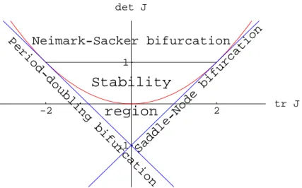
2.8 The occurrence of the three main types of bifurcation for two-dimensional

(16)

2.9 The presence of subcritical bifurcation in the autonomous Ricker type

competi-tion model (2.1) . . . 58

2.10 Four different scenarios in which an individual Ricker competition map Fi has

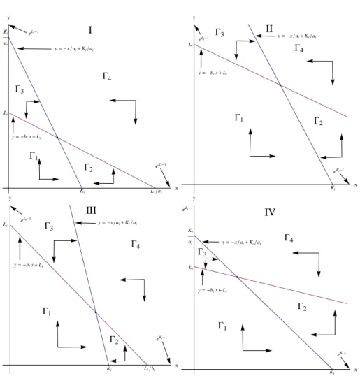
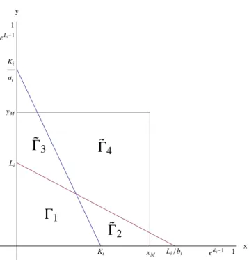
a maximum value on the axes. The values of the competition parameters are fixed such thatab< 1. In these curvesa= b=1/2. . . 61 2.11 The position of the isoclines and the setsΓ1,Γ2,Γ3andΓ4, in the first quadrant,

for each one of the four situations in which the mapFi has the maximum value

on the axes. I-eKi−1 _< _L

i/bi andeLi−1 < Ki/ai; II -eKi−1 > Li/bi and eLi−1 >

Ki/ai;III-eKi−1> Li/biandeLi−1< Ki/ai; andIV-eKi−1 < Li/biandeLi−1 > Ki/ai. 62

2.12 The sets and the isoclines when the maximum of the mapFi is less than one . . 64

2.13 The progress of the Schwarzian derivative of the two-periodic one-dimensional Ricker mapΦ₂at (x0) when the parametersλ0andλ1are on the period doubling

bifurcation curves. . . 72

2.14 The bifurcation scenario in the parameter space of the mapΦ2 =R1◦R0. . . . 73

2.15 The bifurcation scenario of the 2₋periodic Ricker competition equation in the

parameter space (K0,K1) when the carrying capacityLand the competition

pa-rametersaandbare fixed. . . 74

2.16 The bifurcation scenario of Eq. (2.34) in the parameters space (K0,L0) when

K1 =1/2,L1 =1/10, anda=b=1/2. . . 75

2.17 Some examples of the bifurcation scenario of Eq. (2.34) in the parameter space (K0,L0). . . 76

2.18 The fitness function. . . 79

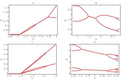
2.19 The phase-space diagram for the exclusion fixed point (a−_a1,0) of the logistic

competition model. A - The exclusion fixed point is asymptotically stable:a =

2.5,b=1.01,c= 0.3,d= 0.1. B - The exclusion fixed point is a saddle:a= 2, b=1.1,c=0.3,d= 0.1. C - The exclusion fixed point is asymptotically stable:

a = 3, b = 1.01, c = 0.3, d = 0.1, where the center manifold is stable on the

x₋axis. D - The exclusion fixed point is a saddle: a = 2.5, b = 1.06, c = 0.3,

d = 0.1 where the center manifold is unstable on the x₋axis and in the interior

of the first quadrant. . . 81

2.20 The existence of an exclusion asymptotically stable 2₋periodic cycle on the

x₋axis of the logistic competition model when one eigenvalue is outside the

unit circle and the second eigenvalue is inside the unit circle. . . 82

2.21 The stability of the exclusion fixed points and the validity of the exclusion prin-ciple in the logistic competition model. A - If 1<a_≤ 3 andb< 1+d(a−_a1)(or

b−1 d <

a−1

a ), then ( a−1

a ,0) is asymptotically stable and speciesygoes extinct. B

-If 1< b_≤ 3 andb > ₁₊c_c₋_a (or b−_b1 > a−_c1), then (0,b−_b1) is asymptotically stable

and speciesxgoes extinct. . . 82

2.22 The stability regions and the bifurcation scenario of the logistic competition

model in the parameter spacea₋b. . . . 84

2.23 Phase-space diagram for the coexistence fixed point of the logistic competition

model. . . 85

2.24 If the carrying capacities K and L are in region S, then the coexistence fixed

point of the autonomous Leslie-Gower model is globally asymptotically stable. If the parameters are in region R and Q, then the exclusion fixed point is globally

(17)

LIST OF FIGURES xvii

3.1 An instance of one unimodal Allee map f. . . 97

3.2 Parts I and II depicts the left and the right preimages of Af undergwhile parts

III and IV depicts the left and the right preimages ofAgunder the map f. . . 99

3.3 Bifurcations curves for the 2₋periodic nonautonomous difference equation with

Allee effects xn+1 =anx2n(1−xn),an+2 =anand xn+2 = xnin the (a0,a1)−plane. . 104

3.4 Progress of the exploitation rate. . . 106

3.5 The progression of the organic composition of the capital in the model (3.20).

In the left plot we fix the parameter b and increase d, while in the right plot

we fixdand increaseb. In both cases, in general, the behaviour of the organic

composition of the capital is similar. As according b or d increases, for low

profits the tendency is decreases the organic composition of the capital, for high profits, the tendency is increases the organic composition of the capital. . . 107

3.6 Zero, one and two positive fixed points for the profit rate whenais respectively,

less thanac, equalac and greater thanac, whereac ≈ 1.64271. . . 109

3.7 Stability of the unique positive fixed point. In the first caser= rcis semi-stable

on the right side and unstable on the left side (rc ≈ 0.478625). In the second

caser= rc is always unstable. . . 110

3.8 Stability of the two positive fixed points. In the first case the 1st positive fixed point is unstable and the 2nd positive fixed point is locally asymptotic stable. In the second case the 2nd positive fixed point is unstable (the 1st positive fixed point is not visible because it is small, but it exists). . . 110

3.9 The Liapunov exponent λof the function fa under the parameter aapplied to

the profit rate. . . 112

3.10 Progress of the topological entropy ht for the model (3.23). According the

growth of the parameterathe topological entropyht increases for values near 1. 113

3.11 The stability region of the 2-periodic cycle for the nonautonomous 2-periodic system in the (a0,a1)-plane. . . 114

3.12 The booming function as a function of the parameter afor different values of

the parameterε. . . 116

3.13 Illustration taken from “http://www.thelongwaveanalyst.ca” that shows the

Kon-dratieffWave periods along with US stocks market, US prices and T-Bond rates. 117

3.14 For a = 1.35 model (3.23) can be interpreted as the Kondratiev waves. The

progression of the profit rate can be viewed in four seasons that repeat each five decades. . . 118

4.1 The presence of strange attractors in the autonomous Ricker competition model

whena = b= 0.5. In plot on the leftK = 3.2 andL = 3.1 while in plot on the

rightK = 3.2 andL= 3.5. . . 120

4.2 The presence of strange attractors in the autonomous logistic competition model

whena= 4.3 andb = 3.9. In plot on the leftc = 0.6 andd =0.2 while in plot

(18)

(19)

Introduction

In population dynamics, and from the mathematical point of view, there are two major modeling

strategies: (i) The continuous time approachusing theory of differential equations; and (ii)

Thediscrete time approach which is more related with the structure of data of a population. Hence, many laws of the nature are intrinsically discrete.

In particular, when we study a mathematical model, one of the main objectives is to give

relevant information/contribution for the importance of the model. Moreover, different

mod-eling strategies with different assumptions to describe particular features of the population, is frequently used among researchers.

Throughout this work we use the discrete time analysis. Hence, this work deals with diff

er-ence equations, or in other equivalent terminology, recursions, iterations and discrete dynamical systems. Such kind of iterative procedures are omnipresent in mathematics, as well in a couple of related sciences such as Biology, Ecology, Economic, Engineering, etc.

There are two main kind of discrete time approach: (i) Theautonomous modelin which the

dynamics of the system is given by the same map. This kind of systems predicts the evolution without considering many changes along the time. In other words, the equation that generate

the system has a constant parameters. (ii) The nonautonomous model, i.e., difference

equa-tions whose right-hand side, explicitly depend on time or change. Hence, seasonal influences,

controlling, external effects, and other mechanisms are allow in nonautonomous models. In

concrete equations the constant parameters are replaced by time-dependent sequence of param-eters.

In this work we have both, autonomous and nonautonomous models. Explicitly, an

au-tonomous difference equation is defined by

xn+1= f(xn),n=0,1,2, . . . . (1)

If x0is the initial population, its evolution along the timenis given by

x1 = f(x0),

x2 = f(x1) = f ◦ f(x0)= f2(x0),

.. . xn+1 = fn(x0),

.. .

As it is clearly seen, the evolution of the population is generated by the same map.

The nonautonomous difference equation is governed by the rule

xn+1= fn(xn),n=0,1,2, . . . . (2)

(20)

Here the evolution of the population is generated by the composition of the sequence of maps f0, f1, f2, . . . .

Explicitly,

x1 = f0(x0),

x2 = f1(x1)= f1◦ f0(x0),

.. .

xn+1 = fn◦ fn−1◦. . .◦ f1◦ f0(x0),

.. .

If the sequence of maps is periodic, i.e., fn+p = fn, for alln = 0,1,2. . . and some positive

integerp> 1, then we talk about nonautonomous periodic difference equations. Systems where

the sequence of maps is periodic model population with fluctuation habitat, and they are com-monly called periodically forced systems. Under this scenario, the evolution of the population is given by

x1 = f0(x0),

x2 = f1◦ f0(x0),

.. .

xp = fp−1◦. . .◦ f1◦ f0(x0),

xp+1 = f0◦ fp−1◦. . .◦ f1◦ f0(x0),

.. .

Throughout this work, the nonautonomous part is about periodic forced systems.

Notice that the nonautonomous periodic difference equation (2) does not generate a discrete

(semi)dynamical system [30] as it may not satisfy the (semi)group property. One of the most effective ways of converting the nonautonomous difference equation (2) into a genuine discrete (semi)dynamical system is the construction of the associated skew-product system as described in a series of papers by Elaydi and Sacker [28, 29, 30, 31]. It is noteworthy to mention that this

idea was originally used to study nonautonomous differential equations by Sacker and Sell [68].

Most of the contents in Chapter 1 is devoted to this theory. We present all the necessary machinery to develop the skew-product system. The principal results and new developments concerning the periodicity of the system and its stability is present. These new developments include results associated with the introduction of the notion of the derivative in the skew-product. Hence a natural extension to nonautonomous periodic systems of the main stability results of autonomous systems is developed. One entire section is about the center manifold and the stable and unstable manifold as well for any nonlinear periodic system. Finally we end the chapter presenting a brief extension of the main results of bifurcation of one-dimensional

au-tonomous maps to periodic equations, i.e., maps with one variable andpparameters. Moreover,

degeneracy conditions for both, variables and parameters is studied.

In Chapter 2 and in Chapter 3 we study some concrete models trying to apply, whenever need, the theory developed in Chapter 1. So Chapter 2 is totally dedicated to the study of the properties of some competition models for two species. Stability, bifurcation and

(21)

INTRODUCTION 3

map. We found out that the new model that we propose, the logistic competition model, ex-hibits a similar behavior than the Ricker competition model. We also turn our attention to the nonautonomous Ricker competition model and to the Leslie-Gower competition model.

In Chapter 3 we study the properties of unimodal Allee maps for both autonomous and nonautonomous systems. The first model is devoted to population dynamics while the second is in economic theory.

(22)

(23)

Chapter 1 Nonautonomous periodic systems

Dynamical systems occur in all branches of science. “The main goal of the study of dynamical systems is to understand the long behavior of states in a system for which there is a determin-istic rule for how a state evolves” (Martin Rasmussen [62]). For this reason “an understanding of the asymptotic behavior of a dynamical systems is probably one of the most relevant prob-lems in sciences based on mathematical modeling” (Christian Potzsche [61]). Hence, one of the mathematical concept of a dynamical system is based on the simple fact that there are cer-tain rules that governs our natural laws. These rules, in general, can be described by discrete mathematical models.

A good example that illustrates what is a discrete dynamical system is the following: “Take a scientific calculator and input any number whatsoever. Then start striking one of the function keys over and over again. . . .For example, if we repeatedly strike theexpkey, given an initial

input x, we are computing the sequence of numbers

x,ex,eex,eeex, . . . .

That is, we are iterating the exponential function.” (Robert Devaney [24]).

In this example the evolution of the system is due to the same function. This is known as an

autonomous discrete dynamical system and it may be defined by the difference equation

xn+1= f(xn),n=0,1,2, . . . .

The evolution here is based in the successive composition of the map f. Hence, a natural

question in the theory of discrete dynamical systems is the following: given an initial valuex0,

what happens to the sequence of iterates

x0, f(x0), f(f(x0)), f(f(f(x0))), . . .?

Notice that this law is time-independent.

However, in many concrete cases, this notion of discrete dynamical system, is not enough to describe real world phenomena. For instance in population dynamics is more realistic to con-sider evolutionary adaptations due the influence of the environment. The appropriate technique to solve such problem is the use of nonautonomous models or time-dependent equations. Such

kind of models can be governed by the difference equation

xn+1= fn(xn),n=0,1,2, . . . .

(24)

According to this law, the evolution is time-dependent because the sequence of functions fi,

i =0,1,2, . . .usually is not equal. In general, this kind of models possesses a parameter which changes in time.

In real world, in general, most of the known phenomena have the tendency to repeat af-ter some time. Here arises the nonautonomous periodic models. According to our af-

termi-nology, in the sequence of functions we have for some integer p > 1, fn+p = fn, for all

n = 0,1,2, . . .. However, the nonautonomous periodic difference equation does not generate

a discrete (semi)dynamical system as it may not satisfy the (semi)group property. This problem was positively solved by Elaydi and Sacker, in a series of articles [28, 29, 30, 31], where these mathematicians developed the theory of skew-product systems.

It should be noted that Ziyad AlSharawi, a former Elaydi’s PhD student, used the skew-product theory in his dissertation [6]. He was able to extend the Sharkovsky’s theorem and its

converse to periodic difference equations. An extension of the well-known Singer’s theorem is

present in [6]. Moreover, AlSharawi did a relevant work in the construction of concrete periodic systems and almost periodic systems according to certain previous properties on the maps.

We are going to use the skew-product theory in another perspective. We focus here in the properties of the stability of the solutions of periodic difference equation. Moreover, we study the bifurcation for such kind of systems.

Hence in Section 1.1 we present the principal definitions and techniques that permit us the

construction of a discrete (semi)dynamical system via the nonautonomous periodic difference

equation.

In Section 1.2 we study some properties of the solutions of the nonautonomous periodic systems and in the next section we focus our attention in its stability. A natural extension of the more common properties of autonomous systems is introduced.

The theory of the center manifold and the stable and unstable manifold for these systems is study in Section 1.4. We introduce techniques that allow us to study the stability of a fixed point, for any non-linear map, when one (or more) of the eigenvalues are on the unit circle.

In Section 1.5 a natural extension to periodic difference equations of the main results of

bifurcation is treated. The techniques are similar to differential equations and are known for

maps with one variable and one parameter. Moreover, degeneracy conditions for both variable and parameters are developed.

1.1 Skew-product Systems

Let X be a topological space andZ _{be the set of integers. A discrete dynamical system (X, π)}

is defined as a map π : X _×Z _→ _X _{such that} _π _{is continuous and satisfies the following two}

properties

1. π(z,0)= zfor allz_∈X,

2. π(π(z,s),t)= π(z,s+t),s,t_∈Z_and_z_∈_X _{(the group property).}

We say (X, π) is a discrete semidynamical system ifZ_{is replaced by}Z+_{, the set of}

nonneg-ative integers, and the group property is replaced by the semigroup property.

Notice that (X, π) can be generated by a mapFdefined asπ(z,n)= Fn_{(z), where}_Fn_denotes

the nthcomposition of the map F. We observe that the crucial property here is the semigroup

(25)

1.1. SKEW-PRODUCT SYSTEMS 7

A difference equation is called autonomous if it is generated by one map such as

zn+1 = F(zn),z∈X,n∈Z+. (1.1)

Notice that for any z0 ∈ X,zn = Fn(z0). Hence, the orbit O(z0) = {z0,z1,z2, . . .}in Eq. (1.1) is

the same as the set_O(z0)= {z0,F(z0),F2(z0), . . .}under the mapF.

A difference equation is called nonautonomous if it is governed by the rule

zn+1 = F(n,zn),n∈Z+, (1.2)

which may be written in the friendlier form

zn+1= Fn(zn),n∈Z+, (1.3)

whereFn(z)= F(n,z),z∈X. Here the orbit of a pointz0is generated by the composition of the

sequence of maps_{Fn}. Explicitly,

O(z0) = {z0,F0(z0),F1(F0(z0)),F2(F1(F0(z0))), ...} = _{z0,z1,z2, ...}.

When Fi = Fimodp, i ∈ Z+ then we say that Eq. (1.3) is p−periodic, where p is the minimal

period.

It should be pointed out here that the nonautonomous difference equation may not generate

a discrete semidynamical system as it may not satisfy the semigroup property. The following example illustrates this point.

Example 1 Consider the two-dimensional nonautonomous difference equation

(xn+1,yn+1)=

(

(₋1)n

(

n+1 n+2

)

xn,

1 n+1yn

)

,n_∈Z+_. _(1.4)

The solution of Eq. (1.4) is

(x_n,yn)=

(

(₋1)n(n2−1) x0

n+1, y0

n!

)

. Letπ((x0,y0),n)= (xn,yn). Then

π(π((x0,y0),m),n) = π

(

((₋1)m(m2−1) · x0

m+1, y0

m!),n

)

=

(

(₋1)n(n2−1)(−1)

m(m−1)

2 · x0

(n+1)(m+1), 1 n!

1 m!y0

)

.

However,

π((x0,y0),m+n)=

(

(₋1)(n+m)(n2+m−1) x0

m+n+1, 1 (m+n)!y0

)

.

Now we are going to present the appropriate framework in which the nonautonomous dif-ference equation generate a discrete semidynamical system.

Consider the nonautonomous difference equation (1.2) where F(n,_·) _∈ C(Z+

×X,X) = C,

C is the space of continuous functions. The spaceC is equipped with the topology of uniform

(26)

be the set of translates, denoted by H, inC. ThenG(n,_·)_∈ ω(_A), the omega limit set of_A, if for eachn_∈Z+_,

|Ft(n,z)−G(n,z)| →0

uniformly forzin compact subsets ofX, ast _{→ ∞}along some subsequence _{tni}. The closure

of_AinCis called the hull of F(n,_·) and is denoted byY =cl(_A)=_H(F).

On the spaceY, we define a discrete semidynamical systemσ:Y_×Z+_→_Y_by_σ(H(n,_·_),_t)₌

Ht(n,·); that isσis the shift map.

Define the composition operatorΦas follows

Φi

n = Fi+n−1◦. . .◦Fi+1◦Fi ≡Φn(F(i,·)).

Wheni=0, we writeΦ0

nasΦn.

The skew-product system is now defined as

π: X_×Y_×Z+ _→_X_×_Y_,

with

π((z,G),n)=(Φ_n(G(i,z)), σ(G,n)). IfG = fi, thenπ((z, fi),n)= (Φin(z), fi+n).

The following commuting diagram illustrates the notion of skew-product systems where

P(a,b)=bis the projection map in the second component.

X_×Y_×Z+ π //

P×id

X_×Y

P

Y_×Z+ _σ //_Y

For eachG(n,_·)_≡gn ∈Y, we define the fiberFg overGasFg =P−1(G). Ifg= fi, we write

Fg asFi.

Theorem 2 [30]πis a discrete semidynamical system.

Example 3 (Example 1 revisited) Let us reconsider the nonautonomous difference equation

(xn+1,yn+1)=

(

(₋1)n

(

n+1 n+2

)

xn,

1 n+1yn

)

,(x(0),y(0))=(x0,y0),n∈Z+.

Hence,

F(n,x,y)=

(

(₋1)nn+1 n+2x,

1 n+1y

)

= fn(x,y)=(f1,n(x), f2,n(y)).

Its omega limit set is given by G(n,x,y) = ((₋1)n_x,_{0), that is, g}

n is a periodic sequence given

by g0 =g2n, g1= g2n+1, for all n∈Z+, in which g0(x,y)=(x,0), and g1(x,y)=(−x,0).

It is easy to verify that π defined as π((x,y, fi),n) = (Φin(x,y), fi+n) is a semidynamical

system, i.e, the map

π((x,y, fi),n) =

    

(₋1)in+n(n2−1) i+1

i+n+1x,

1

∏n−1

j=0(i+1+ j)

y

  ,

(

(₋1)(n+i)n+i+1 n+i+2x,

1 n+i+1y

)_

(27)

1.2. PERIODICITY 9

1.2 Periodicity

In this section our focus will be on the p₋periodic nonautonomous difference equation of the

form

zn+1= Fn(zn),n∈Z+, (1.5)

wherez_∈X, Fi = Fimodp,i∈Z+withFi ∈X, where pis the minimal period of the equation.

Recall thatz∗ is a fixed point of the autonomous equationzn+1 = F(zn) ifF(z∗) = z∗andz∗

is a fixed point of the nonautonomous equation (1.5) if it is a fixed point for all the maps, i.e., Fi(z∗)= z∗,∀i∈Z+.

We begin by defining anr₋periodic cycle.

Definition 4 An ordered set of points Cr= {z0,z1, . . . ,zr−1}is an r−periodic cycle in X if

F(i+nr) modp(zi)=z(i+1)mod r,n∈Z+.

In particular,

Fi(zi)=zi+1,0≤i≤ r−2,

and

Ft(ztmodr)=z(t+1) modr,r−1≤t ≤ p−1.

It should be noted that ther₋periodic cycleCr in X generates an s−periodic cycle on the

skew-productX_×Y (Y = _{F0,F1, . . . ,Fp−1}) of the form

b

Cs= {(z0,F0),(z1,F1), ...,(z(s−1) modr,F(s−1) modp)},

wheres= lcm[r,p] is the least common multiple ofrand p.

To distinguish these two cycles, ther₋periodic cycleCronXis called anr−geometric cycle

(or simplyr₋periodic cycle when there is no confusion), and thes₋periodic cycleCbsonX×Y

is called ans₋complete cycle.

Example 5 Letα, β_∈(0,1)withα, βand define

fn(x,y)=

    

1+α(1+ x₋y)if n =0 mod 4

α(₋1+ x+y)if n=1 mod 4

1+β(1+x₋y)if n= 2 mod 4

β(₋1+x+y)if n= 3 mod 4 ,

and

gn(x,y)=

    

β(₋1+x+y)if n=0 mod 4

1+β(1₋ x+y)if n=1 mod 4

α(₋1+x+y)if n =2 mod 4

1+α(1₋x+y)if n =3 mod 4

,

n_∈Z+_{. This leads to a}₄₋_{periodic two-dimensional nonautonomous di}_ff_{erence equation. There}

is, however, a 2₋periodic geometric cycle, namely, C2 = {(0,1),(1,0)} (see Fig. 1.1). This

periodic cycle in the space R2

+ generates the following 4−complete cycle in the skew-product

R2

+×Y

b

C4= {((0,1),(f0,g0)),((1,0),(f1,g1)),((0,1),(f2,g2)),((1,0),(f3,g3))},

(28)

Figure 1.1: A 2₋periodic geometric cycle onX=R2

+and a 4−periodic complete cycle on the skew productX×Y

whereY=_{F0,F1,F2,F3},Fi=(fi,gi),i=0,1,2,3 for the difference equation defined in example 5.

We are going to provide a deeper analysis of the preceding example. Letd = gcd(r,p) be

the greatest common divisor ofrand p, s= lcm[r,p] be the least common multiple ofrand p,

m= p

d,andℓ = s

p.The following result is crucial in the setting of periodic cycles. It is published

in [29] for a general metric space.

Lemma 6 [29] Let Cr ={z0,z1, . . . ,zr−1}be a set of points in X. Then the following statements

are equivalent.

1. Cr is a periodic cycle of minimal period r.

2. For0_≤i_≤ r₋1, F(i+nd) modp(zi)=z(i+1) modr.

3. For0_≤i_≤ r₋1, we have that

Fimodp(zimodr)= F(i+d) modp(zimodr)=. . .= F(i+(m−1)d)mod p(zimodr)= z(i+1) modr;

Fimodp(z(i+d) modr)= F(i+d) modp(z(i+d) modr)=. . . = F(i+(m−1)d)mod p(z(i+d) modr)=z(i+d+1) modr;

.. .

Fimodp(z(i+(ℓ−1)d) modr)= F(i+d) modp(z(i+(ℓ−1)d) modr)= . . .= F(i+(m−1)d)mod p(z(i+(ℓ−1)d) modr)=

z(i+(ℓ−1)d+1) modr.

LetK_{denote either}Rq_orCq _{and let us write the parameter family of maps}_F_i_{(z) as}_F_i_(α,_z),

i _∈ Z+_{, where}_α _∈ K _{is a parameter vector and}_z _∈ _{X. The following definition is used in the}

sequel.

Definition 7 Fi :K×X→ X, i∈Z+, is one to one with respect to the parameter vectorαif for

α,bαone has F(α,z), F(_bα,z),_∀z_∈X (with exception of the fixed points). As an example, the nonautonomous Ricker competition model given by

(

xn+1

yn+1

)

=

(

xneKn−xn−anyn

yneLn−yn−bnxn

)

,n_∈Z+_,

whereKn >0 andLn >0 are the carrying capacities of speciesxandy, respectively, andan> 0

and bn > 0 are the competition parameters of speciesyand x, respectively, is one to one with

respect to the carrying capacities parameter vector (fixing the competition parameters). For instance, from the following identity

(

xeK0−x−ay

yeL0−y−bx

)

=

(

xeK1−x−ay

yeL1−y−bx

(29)

1.2. PERIODICITY 11

we conclude thatK0 = K1andL0 = L1. If the carrying capacities are fixed and the competition

parameters vary, then the model still is one to one with respect to the competition parameter vector.

As a consequence of Definition 7 the map is one to one with respect to the parameter vector if it is a one parameter vector family of maps. This observation motivates the following result.

Theorem 8 Suppose that F(α,z), α _∈ K_,_z _∈ _{X, n} _∈ Z+ _{is a one parameter vector family of}

maps one to one inαand write the nonautonomous difference equations as

zn+1 =Fn(αn,zn), (1.6)

in which Fn= Fnmodp, n∈Z+. If the p−periodic difference equation (1.6) with minimal period

p has a nontrivial periodic cycle of minimal period r, then r=t p, t_∈Z+_.

Proof. Suppose that the Eq. (1.6) has a periodic cycle Cr= {z0,z1, . . . ,zr−1}

of periodr , t p,t _∈Z+_{. Let}_d ₌ _gcd(r,_p), _s ₌ _lcm[r,_p], _m ₌ p

d, andℓ = s

p. Thend < p. By

Lemma 6, we have that

F0(α0,z0)= Fd(αd,z0)= . . .= F(m−1)d(α(m−1)d,z0)=z1;

F0(α0,zd)=Fd(αd,zd)=. . . = F(m−1)d(α(m−1)d,zd)=zd+1;

.. .

F0(α0,z(ℓ−1)d)= Fd(αd,z(ℓ−1)d)= . . .= F(m−1)d(α(m−1)d,z(ℓ−1)d)=z(ℓ−1)d+1.

Since the maps are one to one in the parameter vector, they do not intersect, unless they are equal. Similarly, one may show that Fi = Fi+d = . . . = Fi+(m−1)d, i ∈ Z+. This implies that Eq.

(1.6) is of minimal periodd, a contradiction.

As we remarked earlier if thep₋periodic nonautonomous difference equation has a periodic

cycle of minimal period r, then the associated skew-product system π has a periodic cycle of

period s = lcm[r,p] (s₋complete cycle). There are p fibers_Fi = P−1(Fi). Are the s periodic

points equally distributed on the fibers?

Before giving the definitive answer to this question, let us examine the diagram presented in

Fig. 1.2 in which p= 9, andr= 6.

There are two points on each fiber. The graphs F0, F3, and F6 intersect at the two points

(z0,z1), (z3,z4); the graphs F1,F4, and F7 intersect at the two points (z1,z2), (z4,z5); and the

graphsF2,F5,F8intersect at the points (z2,z3), (z5,z0).

Note that the number of periodic points on each fiber is 2, which isℓ = lcm[r_p,p]. The following crucial lemma proves this observation.

Lemma 9 [28] The orbit of (zi,Fi) in the skew-product system intersects each fiber Fj, j =

(30)

Figure 1.2: A 6−periodic cycle in a 9−periodic system.

1.3 Stability

Let λ1, λ2, . . ., λq be the (real or complex - not necessary different) eigenvalues of the real or

complex matrixAq×q. The spectral radius of the matrixAis given by

ρ(A)=max_{|λi|: 1≤i≤q}.

It is well known that the fixed pointz∗ of the autonomous equation (1.1) is asymptotically

stable (respectively unstable) if ρ(JF(z∗)) < 1 (respectivelyρ(JF(z∗)) > 1), where JF(z∗) is the Jacobian ofFevaluated atz∗.

In particular, when q = 2, i.e., when (x∗,y∗) is a fixed point of the two dimensional au-tonomous equation (1.1), it is known [26, pp 200] thatρ(JF(x∗,y∗))< 1 if and only if

|tr(JF(x∗,y∗))_{| −}1<det(JF(x∗,y∗))<1, (1.7)

wheretranddetdenote the trace and the determinant of the matrix, respectively, andJF(x∗_,_y∗₎

is the Jacobian evaluated at the fixed point (x∗,y∗). Using the trace-determinant analysis, in [26]

the author presents a complete stability analysis for 2₋dimensional systems.

In Section 1.4 we will present the techniques necessary to determine the stability of the fixed pointz∗whenρ(JF(z∗))= 1 for non-linear maps.

On the spaceXifCr= {z0,z1, . . . ,zr−1},r >1, is anr−periodic cycle of Eq. (1.1), then it is

asymptotically stable if

ρ

  

0

∏

i=s−1

JF(zimodr)

 

<1, (1.8)

where JF(zimodr) is the Jacobian evaluated along the periodic orbitCr.

From linear algebra, recall thatρ(A)_{≤ ||}A_||for any norm, whereAis aq_×qreal or complex

matrix, but equality does not necessarily hold. Indeed, for a given norm there are matrices A

such that ρ(A) and _||A_|| may be arbitrarily far apart. On the other hand, there is a result that shows that, for a given matrixAwe can always find some norm such that_||A_||is arbitrarily close toρ(A) (for more details about this point see [59]). In our context it says that for anyϵ >0 there is a norm_{|||· |||}onRq_(orCq_{) such that}

|||

0

∏

i=s−1

JF(zimodr)||| ≤ρ

  

0

∏

i=s−1

JF(zimodr)

(31)

1.3. STABILITY 13

Takingϵ so small as we want, under condition (1.8), it is possible to find a norm_{|||· |||}such that

|||

0

∏

i=s−1

JF(zimodr)|||<1.

Notice that ifA1,A2, . . . ,Anareq×qmatrices, thenA1A2. . .Anand the cyclic permutations

Aj+1. . .AnA1. . .Aj have the same set of eigenvalues, where 1 ≤ j ≤ n(see [4]). Thus each of

thermatrices of the permuted Jacobian products has the same set of eigenvalues. Consequently,

the order of the products in∏0_i₌_r₋₁JF(xi,yi) is irrelevant for the spectral radius.

We now study stability of the nonautonomous equation. We start by the basic definitions of stability.

Definition 10 Let Cr= {z0,z1, . . . ,zr−1}be an r−periodic cycle in the p−periodic equation (1.5)

in a metric space(X,d), and sb =lcm[r,p]be the least common multiple of p and r. Then 1. Cris stable if givenϵ >0, there existsδ >0such that

b

d(z0,zimodr)< δimpliesbd(Φins(z0),Φins(zimodr))< ϵ,

for all n_∈Z+_{, and}₀

≤ i_≤ p₋1. Otherwise, Cris said unstable.

2. Cris attracting if there existsη >0such that

b

d(z0,zimodr)< ηimplies lim n→∞Φ

i

ns(z0)=zimodr,

for all n_∈Z+_{, and}₀

≤ i_≤ p₋1.

3. We say that Cr is asymptotically stable if it is both stable and attracting. If in addition,

η=_∞, Cris said to be globally asymptotically stable.

Before we present an immediate (basic) consequence of this definition let us recall the chain rule for vector maps which is well known but not used frequently. It says that the Jacobian matrix of the composition of maps is the product of the Jacobian matrices of the maps. In our notation, let us to write z _∈ X as (z1,z2, . . . ,zq) and each map Fn ∈ X as (Fn1,F2n, . . . ,F

q n) ,

n_∈Z+_{. For each 0} _≤_i_≤ _p₋_{1 we write the Jacobian of the composition operator}Φi

mas

JΦi_m(z)= ∂(Φ 1,i

m,Φ2m,i, . . . ,Φ q,i m)

∂(z1_,_z2_{, . . . ,}_zq₎ =

    

∂(Φ1m,i)

∂z1 . . . ∂(Φ1m,i)

∂zq

..

. . .. ... ∂(Φqm,i)

∂z1 . . . ∂(Φqm,i)

∂zq

     .

Using the chain rule this last matrix is equivalent to

    

∂F1

m+i−1 ∂Φ1,i

m−1

. . . ∂F

1

m+i−1 ∂Φq_m,i

−1

..

. . .. ... ∂Fq_m₊_i

−1 ∂Φ1,i

m−1

. . . ∂F

q m+i−1 ∂Φq_m,i

−1     ×. . .×     

∂F1

i+1 ∂Φ1,i

1

. . . ∂F

1

i+1 ∂Φq₁,i

..

. . .. ... ∂F_iq₊₁

∂Φ1,i

1

. . . ∂F

q i+1 ∂Φq₁,i

    ×     

∂F1

i

∂z1 . . . ∂F1

i

∂zq

..

. . .. ... ∂F_iq

∂z1 . . . ∂Fq_i

∂zq

     , or

JFm+i−1

(

Φi_m₋₁(z))_×. . ._×JFi+1

(

Φi₁(z))_× JFi(z).

Thus,

JΦi_m(z)= 0

∏

j=m−1

JFj+i

(

(32)

Theorem 11 Let X be a metric space induced by the norm _{|||· |||} , Cr = {z0,z1, . . . ,zr−1} be

an r₋periodic cycle of the p₋periodic equation (1.5), and s = lcm[r,p] be the least common multiple of p and r. Then Cris asymptotically stable if|||∏0i=s−1JFi mod p(zimodr)|||<1.

Proof. From the hypothesis the norm of the Jacobian of the composition operator is upper bounded by one, i.e., there exists an open sphereSϵ(zimodr) with centerzimodrand radiusϵsuch

that

|||JΦi_s(z)_{||| ≤} M <1,_∀z_∈Sϵ(zimodr).

Then using the mean value theorem for vector-valued function we have

|||Φi_s(z0)−Φis(zimodr)||| ≤ M||z0−zimodr|||,

for 0 _≤i_≤ p₋1,z0 ∈Sϵ(zimodr), or equivalently,

|||Φi_s(z0)−zimodr||| ≤ M|||z0−zimodr|||.

Since M< 1 the last inequality implies thatΦi

s(z0)∈Sϵ(zimodr), 0≤ i≤ p−1. Using the same

argument one obtain

|||Φi_2s(z0)−zimodr||| ≤ M2|||Z0−zimodr|||.

By induction we can prove that

|||Φi_ns(z0)−zimodr||| ≤ Mn|||z0−zimodr|||,∀n∈Z+. (1.9)

This implies that lim

n→∞Φ

i

ns(z0)=zimodr, 0≤i≤ p−1. ThusCris attracting.

To see the stability ofCrnote that the following relation holds

zimodr= Φins(zimodr),∀n∈Z+.

Consequently the relation (1.9) is equivalent to

|||Φi_ns(z0)−Φins(zimodr)||| ≤ Mn|||z0−zimodr|||,

0< M< 1 and 0_≤i_≤ p₋1. Takingδ < ϵ, for anyϵ >0 we obtain

|||Φi_ns(z0)−Φins(zimodr)||| ≤ Mn|||Z0−Zimodr|||

< Mnδ < Mnϵ < ϵ. ThusCris stable. Consequently,Cris asymptotically stable.

Remark 12 Notice that if z∗ _{is a fixed point of the sequence of maps F}

i, i ≥ 0, i.e., z∗ is a

fixed point of each individual map, then one can adapt the precedent result and show that z∗is asymptotically stable if_|||∏n_i=0JFi(z∗)|||< 1, for all n≥ 0.

Consider the skew-product system π on X _× Y with X a metric space with metricd,b Y =

{F0,F1, . . . ,Fp−1}equipped with the discrete metricd, wheree

e

d(Fi,Fj)=

{

(33)

1.3. STABILITY 15

Define a metricdπ _on_X_×_Y_as

dπ = ((z,Fi),(u,Fj)

)

= d(z,b u)+d(Fe i,Fj).

Let π1(z,F) = π((z,F),1), then πn(z,F) = π((z,F),n). Thus π1 : X _×Y _→ X _×Y is a

continuous map which generates an autonomous system on X_×Y. Consequently, the stability

definitions of fixed points and periodic cycles follow the standard ones that may be found in [24, 26].

Now we give a definition of stability for a complete periodic cycle in the skew-product system.

Definition 13 A complete periodic cycleCbs= {(z0,F0),(z1,F1), ...,(z(s−1) modr,F(s−1)mod p)}is

1. stable if givenϵ > 0, there exitsδ >0, such that

dπ((z0,Fi),(z0,F0))< δimplies dπ(πns(z0,Fi), πns(z0,F0))< ϵ,∀n∈Z

+

. Otherwise,Cbsis said unstable;

2. attracting if there existsη >0such that

dπ((z0,Fi),(z0,F0))< ηimplies lim n→∞π

ns_(z

0,Fi)=(z0, f0);

3. asymptotically stable if it is both stable and attracting. If in addition,η = _∞,Cbs is said

to be globally asymptotically stable.

SinceFi+ns = Fifor alln, it follows from the above convergence thatFi = Fi mod p. Hence,

stability can occur only on each fiberX_{× {}Fi},0≤ i≤ p−1.

It should be noted that one may reformulate Theorem 11 in the setting of the skew-product

system. However, to do so, one needs to develop the notion of derivative in the space X_×Y.

Definition 14 Letπm _: _X

×Y _→ X_×Y defined asπm_(z,_F

i) = (Φim(z),Fi+m). The generalized

derivative ofπmis defined as

D(πm(z,Fi))= JΦim(z)= 0

∏

j=m−1

JFj+i(Φij(z)),

withΦi₀(z)= z. In particular, when X= R_{we write}

D(πm(x, fi))=

d dx(Φ

i m(x))=

(

Φi_m)′(x)= 0

∏

j=m−1

f_j′₊_i(Φi_j(x)),Φi₀(x)= x.

Theorem 15 A complete periodic cycleCbs= {(z0,F0),(z1,F1), ...,(z(s−1) modr,F(s−1)mod p)}of the

skew-product systemπon X_×Y is asymptotically stable if_|||D(πs_(z

imodr,Fi))|||<1.

Proof. The proof is analogous to the proof of Theorem 11 and it will be omitted.

(34)

Theorem 16 [28] Assume that X is a connected metric space and each Fi ∈Y is a continuous

map on X, with Fi+p = Fi. Let Cr = {z0,z1, . . . ,zr−1} be a periodic cycle of minimal period

r of the p₋periodic nonautonomous difference equation (1.5). If Cr is globally asymptotically

stable, then r divides p. Moreover, r = p if the sequence_{Fn}is a one-parameter family of maps

F(αn,z)and F is one to one with respect toα.

Obviously, the stability of the periodic cycle can be studied via the spectral radius because for any matrix Aone hasρ(A)_{≤ ||}A_||for any norm. Thus if

||

0

∏

i=s−1

JFi(zimodr)||<1,

then it follows that all the eigenvalues of∏0_i=s−1JFi(zimodr) lie inside the unit disc.

In general, it is not easy and in most of the concrete cases it is an unknown problem, to

determine the product of the Jacobians along the periodic orbit for nonautonomous difference

equation in higher dimension. If it is possible to determine this product, then we can speak about stability of the cycle whenρ(∏0_i₌_s₋₁JFi(zimodr)

)

<1.

We now consider the particular case whenX =R_{. If}_C_r₌ _{_x₀_,_x₁_{, . . . ,}_x_r₋₁_}_{is an}_r₋_periodic

cycle of the one-dimensional nonautonomous p₋periodic difference equation (1.5), thenCr is

asymptotically stable if

|(Φi_s)′(ximodr)|<1,

and it is unstable if

|(Φi_s)′(ximodr)|>1,

where s is the least common multiple of r and p. Note that ximodr is a fixed point of the

composition operatorΦi

s.

When the periodic cycle is nonhyperbolic the stability criteria are more involved. These cri-teria will be summarized in the next two results. The first treats the case when(Φi_s)′(ximodr)= 1

while the second treats the case (Φi s

)′

(ximodr) = −1. Since the proof follows the same

tech-niques as in [26] for one map we will omit the proof here.

Theorem 17 Let Cr = {x0,x1, . . . ,xr−1}be an r−periodic cycle of the one-dimensional

nonau-tonomous p₋periodic difference equation (1.5) such that(Φi_s)′(ximodr)= 1. If

(

Φi_s)′(x),(Φi_s)′′(x) and(Φi

s

)′′′

(x)are continuous at ximodr, then the following statements hold:

1. if(Φi_s)′′(ximodr), 0, then Cris unstable;

2. if(Φi s

)′′

(ximodr)= 0and

(

Φi s

)′′′

(ximodr)> 0, then Cris unstable;

3. if(Φi_s)′′(ximodr)= 0and

(

Φi_s)′′′(ximodr)< 0, then Crasymptotically stable.

Before present the second case, we need to introduce the notion of theSchwarzian

deriva-tive.

Definition 18 TheSchwarzian derivative, S f , of a C3 function f is defined by

S f(x)= f

′′′_(x)

f′_(x) −

3 2

(

f′′(x) f′_(x)

)2

(35)

1.4. INVARIANT MANIFOLD 17

Theorem 19 Let Cr = {x0,x1, . . . ,xr−1}be an r−periodic cycle of the one-dimensional

nonau-tonomous p₋periodic difference equation (1.5) such that (Φi_s)′(ximodr) = −1. If

(

Φi_s)′(x),

(

Φi s

)′′

(x)and(Φi s

)′′′

(x)are continuous at ximodr, then the following statements hold:

1. if SΦi_s(ximodr)< 0, then Cris asymptotically stable;

2. if SΦi

s(ximodr)> 0, then Cris unstable.

In [22] the authors present a complete classification of nonhyperbolic fixed points for one-dimensional autonomous maps. This classification is still valid for ther₋periodic cycleCr, i.e.,

whenximodris a fixed point of the one-dimensional mapΦis. Hence, replacing the map f byΦis

andx∗byximodrin Fig. 1.20 in [26, page 33] one has a complete classification of nonhyperbolic

periodic points for one-dimensional periodic systems.

1.4 Invariant manifold

In this section we present the appropriate tools that allow us, to compute analytically, the center manifold and the stable and unstable manifold for any nonlinear map near the fixed point. It should mention that this section is based on our article [48].

Let F : Rk _→ Rk _{be a map such that} _F _∈ _C2 _and _F(0) ₌ _{0. Then one may write} _F _{as a}

perturbation of a linear mapL,

F(X)= LX+R(X), (1.10)

where Lis ak_×kmatrix defined byL = D(F(0)),R(0) = 0 and DR(0) = 0, where Ddenotes

the Jacobian matrix. Now we will introduce special subspaces ofRk_{, called invariant manifold}

[77], that will play a central role in our study of stability and bifurcation.

An invariant manifold is a manifold embedded in its phase space with the property that it

is invariant under the dynamical system generated by F. A subspace M of Rk _{is an invariant}

manifold if whenever X _∈ M, thenFn_(X)

∈ M, for alln _∈Z+_{. For the linear map}_{L, one may}

split its spectrum σ(L) into three setsσs, σu, and σc, for whichλ ∈ σs if |λ| < 1, λ ∈ σu if

|λ_|>1, andλ_∈σcif|λ|=1.

Corresponding to these sets, we have three invariant manifold (linear subspaces) Es, Eu,

andEc _{which are the generalized eigenspaces corresponding to}_σ

s,σu, andσc, respectively. It

should be noted that some of these subspaces may be trivial.

The main question here is how to extend this linear theory to nonlinear maps. Corresponding to the linear subspacesEs_, _Eu_{, and}_Ec_{, we will have the invariant manifold the stable manifold}

Ws_{, the unstable manifold}_Wu_{, and the center manifold}_Wc_.

The center manifold theory [9, 10, 40, 52, 76, 77] is interesting only if Wu ₌ _{₀_}_{. For in}

this case, the dynamics on the center manifoldWc determines the dynamics of the system. The

other interesting case is whenWc ₌

{0_}and we have a saddle. LetEs

⊂ Rs_, _Eu

⊂ Ru_{, and} _Ec

⊂ Rt_{, with} _s₊_u₊_t ₌ _{k. Then one may formally define the}

above mentioned invariant manifold as follows:

Ws(0)= _{x_∈Rk_|_Fn_(x)_→_0,_n_{→ ∞}}_,

and

Wu(0)= _{x_∈Rk_|∃{_q_n_}∞

(36)

It is noteworthy to mention that the center manifold is not unique, while the stable and unstable manifold are unique.

The next result summarizes the basic invariant manifold theory

Theorem 20 (Invariant manifold theorem) [39, 52] Suppose that F _∈ C2_{. Then there exist}

C2 _{stable W}s _{and unstable W}u _{manifold tangent to E}s _{and E}u_{, respectively, at X} ₌ ₀_{and C}1

center manifold Wc tangent to Ec at X = 0. Moreover, the manifold Wc, Ws and Wu are all invariant.

Before embark in the main aim of this section, notice that the techniques that we are going to develop in the next subsections can be applied to nonautonomous periodic systems in higher

dimension. To do that is enough to replace the map F by the composition operatorΦi_s, where

sis the least common multiple of pandr, with pthe minimum period of the system andrthe

minimum period of the cycle.

In working with concrete maps, as we remarked earlier, is not easy to find explicitly the product of the Jacobians along the periodic orbit.

1.4.1 Center manifold

Let us first focus on the case when σu = ∅. Hence the absolute value of the eigenvalues of L

are less or equal to one. By a suitable change of variables, one may represent the map Fas the

following system of difference equations

{

xn+1 = Axn+ f(xn,yn)

yn+1 = Byn+g(xn,yn)

. (1.11)

First we assume that all eigenvalues of At×t are on the unit circle and all the eigenvalues ofBs×s

are inside the unit circle, witht+ s=k. Moreover,

f(0,0)=0,g(0,0)= 0,D f(0,0)=0 andDg(0,0)= 0.

SinceWc _{is tangent to} _Ec ₌ _{_(x,_y) _∈ _Rt _×_Rs_|_y ₌ ₀_}_{, it may be represented locally as the}

graph of a functionh:Rt _→Rt _{such that}

Wc =_{(x,y)_∈Rt_×Rs_|_y₌_h(x),_h(0)₌_0,_Dh(0)₌_0,_|_x_|_{< δ}_}_,

for a sufficiently smallδ.

Furthermore, the dynamics restricted toWc_{is given locally by the equation}

xn+1 =Axn+ f(xn,h(xn)),x∈Rt. (1.12)

The main feature of Eq. (1.12) is that its dynamics determine the dynamics of Eq. (1.11).

So if x∗ = 0 is a stable, asymptotically stable, or unstable fixed point of Eq. (1.12), then the

fixed point (x∗,y∗)=(0,0) of Eq. (1.11) possesses the corresponding property.

To find the mapy=h(x), we substitute foryin Eq. (1.11) and obtain

{

xn+1 = Axn+ f(xn,h(xn))

yn+1= h(xn+1)=h(Axn+ f(xn,h(xn)))

Nonautonomous Di ﬀerence Equations with Applications