M
ASTER
F
INANCE
M
ASTER
’
S
F
INAL
A
SSIGNMENT
THESIS
ANALYSIS OF PORTFOLIO INSURANCE STRATEGIES
BASED UPON EMPIRICAL DENSITIES
RICARDO JORGE DA GRAÇA RODRIGUES DE ALMEIDA
M
ASTER IN
F
INANCE
M
ASTER
’
S
F
INAL
A
SSIGNMENT
THESIS
ANALYSIS OF PORTFOLIO INSURANCE STRATEGIES
BASED UPON EMPIRICAL DENSITIES
R
ICARDOJ
ORGE DAG
RAÇAR
ODRIGUES DEA
LMEIDAG
UIDANCE:
Professor Dr. Raquel M. Gaspar
1
This study evaluates the performance of the most common Portfolio Insurance
Strategies based on a block-moving bootstrap simulation. We consider not only the
traditional mean-variance approach, but also some measures of downside risk and
stochastic dominance. We find that CPPI 1 should be preferred in terms of stochastic
dominance. We also find that SLPI is constantly dominated by all the other strategies
and a floor of 100% should be preferred to lower ones. Consistently, and purely in terms
of performance analysis, CPPI 3 tends to outperform other strategies.
During this analysis, we try to provide another insight into the controversy over
Portfolio Insurance strategies, turning the decision-making process for future investors
more efficient.
JEL Classification: C15, C60, D81, G01, G11, G15, G23.
Keywords: Portfolio Insurance, Constant Proportion Portfolio Insurance, Option Based Portfolio Insurance, Stop-‐loss Portfolio Insurance, Moving Block Bootstrap.
In the present work, many were the people who have helped me throughout, so I would like to acknowledge those who were essential.
First of all, I am grateful to my supervisor Raquel M. Gaspar who suggested this theme and for the wise clarifications concerning the financial properties of these investments. I would also like to thank her for the patience that she had during the last months.
I am also grateful to Geraldo Chan and Yolanda Gonzalez from Bloomberg London who gave me some of the financial wealth data used in this study.
In addition I would like to thank Jorge Jardim Gonçalves and José Veiga Sarmento, my supervisors at BPI Asset Management for the time they gave me to perform this analysis, and to Isabel Trancoso and my colleagues for their useful comments on earlier drafts of this thesis.
Este estudo avalia a performance das mais comuns estratégias de Portfolio Insurance,
baseando essa análise em simulações de blocos móveis de Bootstrap.
Nesta análise consideramos não apenas as tradicionais medidas associadas à Teoria
Média-variância, mas também outras medidas associadas ao Downside Risk, bem como
classificações de dominância estocástica. Foram identificadas evidências que suportam
que a estratégia CPPI 1 deve ser preferida em termos da sua dominância face às
restantes. Contrariamente, a estratégia SLPI deverá ser preterida face a outras
estratégias de Portfolio Insurance. Encontrámos igualmente evidências de que deverão
ser escolhidas barreiras mínimas mais elevadas, com o objectivo de maximizar a
utilidade da generalidade dos investidores. Consistentemente, e meramente em termos
de performance, a estratégia CPPI 3 é aquela que apresenta resultados mais satisfatórios.
Ao longo desta análise, tentamos proporcionar uma nova visão sobre as controversas
estratégias de Portfolio Insurance, tentando tornar mais eficiente a decisão de futuros
1 Introduction ... 1
2 Overview of the Literature ... 2
2.1 Portfolio Insurance ... 2
2.1.1 Constant Proportion Portfolio Insurance ... 2
2.1.2 Option-based Portfolio Insurance ... 6
2.1.3 Stop-loss Portfolio Insurance ... 7
2.2 Stochastic Dominance ... 8
5.2.1 First order stochastic dominance ... 9
5.2.2 Second-Order stochastic Dominance ... 10
5.2.3 Third-order Stochastic Dominance ... 11
3 Data Analysis ... 12
4 Methodology ... 14
4.1 Moving Block Bootstrap ... 14
4.2 Simulation setup ... 15
5 Results ... 18
5.1 Performance Analysis ... 18
5.1.1. Mean-Variance ... 18
5.1.2. Ratio Analysis ... 21
5.3 Statistical Analysis ... 23
5.4 Other Measures ... 24
5.5 Stochastic Dominance Analysis ... 28
5.5.1. Testing stochastic dominance ... 28
6 Conclusions and further research ... 30
Figure 1: Simulated behaviour for a standard CPPIn strategy ... 5
Figure 2: Simulated behaviour for a standard CPPIn strategy ... 8
Figure 3: Returns distribution for NIKKEI225. ... 12
Figure 4: Returns distribution for S&P500. ... 13
Figure 5: Returns distribution for EuroStoxx 50. ... 13
Figure 6: Payoff function for CPPI 3 (A), CPPI 5 (B) and SLPI (C) with floor equals to (1) 80% and (2) 100% (DJ EuroStoxx50). ... 25
Figure 7: Payoff function for CPPI 3 (A), CPPI 5 (B) and SLPI (C) with floor equals to (1) 80% and (2) 100% (NIKKEI 225). ... 26
Figure 8: Payoff function for CPPI 3 (A), CPPI 5 (B) and SLPI (C) with floor equals to (1) 80% and (2) 100% (NIKKEI 225). ... 27
Index of Tables
Table A: Annualized Expected Returns and Volatilities ... 19Table B: Average Sharpe Ratio, Sortino Ratios and Omega Ratios ... 22
Table C: Relative Skewness ... 24
Table D: Relative Kurtosis ... 24
Table E: StochasticDominance Test for EuroStoxx50 ... 28
Table F: Stochastic Dominance Test for NIKKEI225 ... 28
1
Introduction
In the years before the 2008 crisis, private arrangements have become more and more
important in financial markets. During this period, many investors put their money in
financial assets that should provide protection against market falls and guarantee the
upside potential. However, after the recovery of the markets in 2009, many of these
investors started to ask why their assets didn´t grow with the market – they had the same
investment, Portfolio Insurance instruments (PI).
Traditionally, costumers demand a guaranteed minimum performance for their invested
money. In order to guarantee this goal, offering-banks and insurance companies designed
instruments that could fulfil this purpose, providing the ability to limit downside risk in
bearish markets. Portfolio Insurance instruments could be divided into three categories:
Constant Proportion Portfolio Insurance, Option Based Portfolio Insurance and Stop-loss
Portfolio Insurance.
In this study, we will try to analyse if these types of instruments really do what they
should do – protection – and if they can outperform the payoff provided by traditional
investment strategies such as the buy-and-hold strategy. To perform this analysis we used
both performance measures and stochastic dominance criteria.
This thesis is organised as described ahead. In Chapter 2, we discuss the different PI
strategies and the main advances in this area. Chapter 3 describes some data analysis.
Chapter 4 presents the methodology. Chapter 5 describes the empirical setup and the
simulation results and Chapter 6 presents the main conclusions and some clues for further
2
Overview of the Literature
2.1Portfolio Insurance
The main goal of a risk-averse economic agent is to reduce future uncertainty. Portfolio
Insurance Strategies are investment schemes where the total amount (or, at least, the
major part) of the initial investment is guaranteed in the future.
The first approach to portfolio insurance strategies was developed in the early eighties by
Leland and Rubinstein (1988), who analysed the portfolio insurance techniques based on
the options pricing formula of Black and Scholes (1973). The underlying idea of these
strategies is to provide protection against potential market losses, while preserving the
upward potential (see e.g. Grossman and Villa (1989) and Basak (2002)), allowing
participation in market rallies. Thanks to a dynamic allocation strategy, the portfolio is
protected against market falls by a guaranteed floor, which preserves a guarantee of a
minimum level of wealth at a specific time horizon.
The most preeminent strategies of portfolio insurance are the Constant Proportion
Portfolio Insurance (CPPI), the Option-based Portfolio Insurance (OBPI), and the
Stop-loss Portfolio Insurance (SLPI). From a micro-economic perspective, such strategies
using insurance properties that are thus rationally preferred by individuals that are
specially concerned with the potential losses represented on the left side of the returns
distribution function.
2.1.1 Constant Proportion Portfolio Insurance (CPPI)
Among the most popular strategies of portfolio insurance, the Constant Proportion
markets. The CPPI method was first introduced by Perold (1986) (see also Perold and
Sharpe (1988)) for fixed income instruments and Black and Jones (1987) for equity
markets. CPPI strategies are very popular, commonly used by hedge funds, and are held
essentially for portfolio protection.
This strategy is based on a specific simplified method of dynamic allocation on the risky
asset, denoted S, and a risk-free asset2, denoted B, over time, in order to guarantee a
predetermined floor, which should be equal to the lowest acceptable value of the portfolio
at maturity. The properties of the strategy are extensively studied in the literature (see,
e.g. Black and Rouhani (1989), Black and Perold (1992) and Bookstabber and Langsam
(2000)).
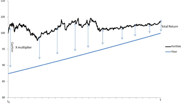
As explained before, the underlying idea of the CPPI strategy consists of managing a
dynamic portfolio, to guarantee at maturity that the portfolio terminal value, denoted by
V
T CPPI
, lies above the guaranteed level defined at t0, denoted K, function of the initial
investment, denoted V0CPPI, as shown below:
CPPI CPPI
T K V
V ≥ × 0
Let F
t;0≤t≤T denote the present value of the guarantee, the so-called floor. This value
should be discounted at a risk-free rate, as shown by:
) ( 0 0 t T r CPPI t CPPI
T K V F K V e
F = × ⇒ = × × − −
The surplus of the current portfolio value VtCPPI, denoted C
t, over the floor Ft is called
cushion, and its value at time t (t Є [0,T]) is given by:
2 This instrument is usually a liquid instrument with residual risk, such as Treasury bills or other liquid
money market instruments;
(1)
[
0]
max t,CPPI t
t V F
C = −
This cushion is the total amount that the investor can use to expose himself to risky
assets. This value can be leveraged over the introduction of a multiplier, denoted m,
which is a constant function of the cushion [C
t]. The portfolio volatility is crucially
dependent upon this parameter, which influenced the payoff function, turning it convex
(only if m satisfies the condition m≥1). As the multiple is higher, larger is the portfolio
value in a bullish market tendency. Nevertheless, the higher the multiple, the faster the
portfolio will approach the floor when there is a decrease in the value of the risky asset.
Usually, this multiple tends to be unconditional (see, e.g. Bertrand and Prigent (2005) and
Prigent and Tahar (2005)), which means that the multiple must not depend on market
conditions but on investor´s risk tolerance function3. Others (see, e.g. Ameur and Prigent
(2006)) defend that in a time-varying framework, the multiple must be conditionally
determined in order to guarantee that the risk exposure remains constant, but path
dependent from market conditions. This exposure ( , which is the total amount
invested in the risky asset, can be determined by:
Et=m×Ct
[
m≥1]
The remaining part is invested in the risk-free asset:
VRf =V0 CPPI
−Et
As the value of the portfolio approaches the floor, the cushion approaches zero, and the
exposure presented in (4) tends to approach zero as well. In theory, the value of exposure
3 This relation is also true for the floor and the initial cushion, that is also a function of the investor´s risk
(5) (3)
should never be negative. However, this relation is only true if we consider a market with
no jumps, keeping the portfolio value away from falling below the floor. This contingent
question is well known and far presented in the literature (see e.g. Grossman and Villa
(1989)), observed especially during financial crisis, when a very sharp drop in the market
may occur before the investor has the chance to re-balance his position.
The behaviour of these type of strategies is shown on Figure 1.
Figure 1: Simulated behaviour for a standard CPPIn strategy
However, it is important to notice that in this strategy the transaction costs are high, due
to the frequent rebalance of the portfolio´s positions, which can be done daily, weekly or
monthly.
Note that the portfolio value [VtCPPI] is always above (or at least equals) the floor [Ft]
2.1.2 Option-based Portfolio Insurance (OBPI)
The Option-based Portfolio Insurance strategy, commonly designated by OBPI, is a
dynamic portfolio strategy that guarantees a percentage of the initial investment, denoted
by V0OBPI. Dated from the seventies, this strategy was first developed by Leland and
Rubinstein (1976), and consists in maintaining a static position either in options and in
the risk-free asset (1) or in the underlying asset (2).
The first option (1) consists in investing the discounted value of the minimum wealth
required at maturity T in a risk-free asset and with the remaining part purchasing a call
option written on the underlying portfolio, denoted C
t;0≤t≤T, with the strike equal to
αV0OBPI, where α is designated by the minimum percentage of the initial amount that the
agent requires to invest in this strategy. At maturity, the final value of the payoff would
be:
V 0
OBPI
+C
T;Strike=αV
0
OBPI =V0 OBPI
+max V
T OBPI −V 0 OBPI , 0
(
)
=max V T OBPI ;V 0 OBPI(
)
Option (2) consists in investing in the underlying portfolio itself in the risky asset and
buying a European put option, denoted by P
t, with the strike settled equal to the desired
floor at T (i.e. long positions in the put option and in the underlying risky asset). At
maturity, the final payoff is given by (assuming put-call parity):
V 0
OBPI
+P T;Strike=αV
0
OBPI =V0
OBPI
+max V
T OBPI −V 0 OBPI , 0
(
)
=max V T OBPI ;V 0 OBPI(
)
.(7)
The final value at maturity becomes:
V T
OBPI
=K+max 0,S
T −K
(
)
, with K=αV0 OBPI
,
where the minimal level required by the investor can be expressed by:
VTOBPI ≥KT ⇒VTOBPI ≥αV0OBPI.
The main difference between CPPI and OBPI strategies resides on the mechanism of
rebalancing. While CPPI strategy is a investment strategy that requires a continuous
reallocation of the corresponding portfolio in order to keep the linear relation between the
cushion and the floor, the OBPI perform this rebalancing using the delta of the protecting
put option (for analysis of the differences between the two strategies see, e.g. Black and
Rouhani (1989) and Bookstaber and Langsam (2000)).
2.1.3 Stop-loss Portfolio Insurance (SL)
Stop-loss portfolio insurance strategy (SL) is a semi-static method of managing insured
portfolios, where the total initial capital, denoted V 0
SL
, is fully invested in the risky asset
as long as the value lies above the present value, at t, of the floor [Kt ]. Once the
portfolio value drops below the discounted floor, the total amount that was previously
invested at risky asset is reallocated entirely to the risk-free asset, thereby ensuring that
the floor at T [KT] is reached. This guarantees that, at maturity, if the floor is reached
during the time-frame of t
(
0<t<T)
, the final payoff will be:V
T SL
=K×V
0 SL
,
(9)
(10)
as presented below:
Figure 2: Simulated behaviour for a standard CPPIn strategy
Otherwise, if the floor was never reached during the investment time horizon, the
portfolio’s terminal value becomes:
VTSL>K×V0SL.
This suggests that this type of strategies is most appropriate to implement if the investor
expects a bullish market tendency.
2.2 Stochastic Dominance
The common mean-variance approach (Markowit (1987)) is used in finance as a
traditional performance analysis that simplifies the decision between investments.
However, this approach uses only two criteria: the mean that represents expected
outcomes, and the risk, measured as the standard deviations of returns. This allows a
simple trade-off analysis but for more complex decisions, the mean-risk approach may
lead to inefficient conclusions. To address this problem, a good alternative to improve the
investment decision is introduced by stochastic dominance (SD) relations.
The stochastic dominance approach was first developed by Whitmore and Findlay (1978)
based on the majorization theory (Hardly et al. (1934)) for discrete distributions, and was
later extended to the main generic distributions by Hanoch and Levy (1969) and
Royhschild and Stiglitz (1970). Since then, it has been widely used in finance.
The basic approach that tries to rank two or more variables according to special classes of
utility functions using an axiomatic model of risk-averse preferences (Fishburn (1964)).
To rank them, investors should follow von-Neumann-Morgenstern utility functions
assuming that they want to maximise their expected utility.
In the stochastic dominance approach random variables are evaluated by point-wise
comparison of some performance functions, which are constructed from their distribution
functions. The stochastic dominance criteria can be found by comparing the orders of
stochastic dominance.
5.2.1 First order stochastic dominance
The first order stochastic dominance rule was first developed by Quirk and Saposnik
(1962), who established the relationship between returns and investor´s preferences. To
ensure that one or more investments dominate others in terms of stochastic dominance,
the cumulative distribution function of an investment A, denoted FA
( )
X , is always belowThe first performance function, denoted by F
x
(1)
(X) is defined as the right-continuous
cumulative distribution (also known as first order stochastic dominance). This function
can be defined as:
F
x
(1)
(X)=F
x(X)=P x
[
≤X]
, for x Є IRAnd ranked by:
x
FSD
y⇔Fx(1)(X)≤Fy(1)(X), for x Є IR
First-order SD implies that investors prefer higher returns to lower ones, which results in
a utility function with a non-negative first derivative.
5.2.2 Second-Order stochastic Dominance
The Second-order stochastic dominance is the best way to rank the different investments
in terms of risk aversion. The second order dominance is given by the following equation:
F
x
(2 )
(X)= F
x(X)dx
−∞
x
∫
, for X Є IRThe weak relation of the second order Stochastic Dominance is defined as:
x
SSD
y⇔Fx(2 )(X)≤Fy(2 )(X), for X Є IR
For decision making process under risk, when X is preferred to Y under SSD rules, all
risk-averse preference scents prefer the investment X instead of the investment Y,
assuring larger outcomes for the same amount of risk.
(13)
(14)
(15)
5.2.3 Third-order Stochastic Dominance
The third order SD was introduced by Whitmore (1970), and consists of adding the
condition that utility functions have a positive (or null) third derivative.
The third order dominance also follows the previous relation and can be defined as:
F x
(3)
(X)= F x(X)dx
−∞
x
∫
∫
, for X Є IRAnd the third order relation is represented by:
x
TSD
y⇔Fx(3)(X)≤Fy(3)(X), for X Є IR
This relation implies a decreased risk aversion function with the increasing of the level of
wealth.
Thus, if X dominates Y under FSD rules, we can assure that X also dominates Y on the
following orders. If X dominates Y under SSD rules, we also can guarantee that this
relation can be maintained on the following order. On the contrary, if an investment
dominates the other under SSD or TSD, we cannot assure any relationship between the
previous orders.
(17)
3
Data Analysis
The possible benefits of Portfolio Insurance strategies have been recently studied in
academia (see, e.g. Bouyé (2009), for a global overview). Unfortunately, the major part
of these studies dealt with stochastic distributions based on normally distributed functions
(see, e.g. Brooks and Levy (1993) and Costa and Gaspar (2011)). However, it is well
presented in the literature that financial returns are not normally distributed. This tends to
bias the approach influenced by the non-consideration of relative factors i.e. variance
clusters, path-dependency between returns, and fatter tails in the empirical distributions.
In order to overcome these constraints, we focused our study on empirical distributions.
To set these distributions, we performed a statistical analysis to observe their real
distribution shape. For our empirical distributions we used data on historical returns from
July 1 of 2002 and June 30 of 2012. Figures 1 to 3 show the obtained empirical
distributions. 0 100 200 300 400 500 600 700 800
-0.10 -0.05 0.00 0.05 0.10
Series: HISTOGRAM Sample 1 2520 Observations 2454
Mean -6.72e-05 Median 0.000369 Maximum 0.132346 Minimum -0.121110 Std. Dev. 0.015690 Skewness -0.522222 Kurtosis 11.09482
Jarque-Bera 6811.590 Probability 0.000000
0 200 400 600 800 1,000 1,200
-0.10 -0.05 0.00 0.05 0.10
Series: S_P500 Sample 1 2520 Observations 2520
Mean 0.000127 Median 0.000788 Maximum 0.109572 Minimum -0.094695 Std. Dev. 0.013764 Skewness -0.206950 Kurtosis 11.45509
Jarque-Bera 7524.289 Probability 0.000000
Figure 4: Returns distribution for S&P500.
0 100 200 300 400 500 600
-0.075 -0.050 -0.025 0.000 0.025 0.050 0.075 0.100
Series: EUROSTOXX50 Sample 1 2520 Observations 2520
Mean -4.72e-05 Median 0.000454 Maximum 0.102188 Minimum -0.090010 Std. Dev. 0.013719 Skewness 0.134930 Kurtosis 10.40300
Jarque-Bera 5762.117 Probability 0.000000
Figure 5: Returns distribution for EuroStoxx 50.
As shown in the previous distributions, and as suggested in the literature, none of the
financial series associated with our indices of reference follows a normal distribution.
The normal distributions are characterized by the absence of bias (i.e. skewness equals
zero) and the stability of kurtosis (i.e. Kurtosis equals three). However, all these financial
series exhibit excess kurtosis and a residual probability of normality (Jarque-Bera´s Test).
These results support our analysis and are consistent with the findings presented in the
literature, refusing the hypothesis of using a normal distribution to study Portfolio
4
Methodology
4.1 Moving Block Bootstrap
The bootstrap method is a computer intensive method for estimation of parameters and
future distributions by sampling the original time series. It consists of randomly
re-sampling series into a so-called bootstrap sample. The classical bootstrap method was
introduced by Efron (1979), who developed a technique for application in independent
data samples. This approach had a great contribution to academic research since it can
overcome the two main strands commonly indicated for prevision with financial series:
lack of sufficient data and uncertainty in the nature of the data generating process.
However, as believed by most of the academic community, stock returns tend to be
dependent. Hence, the standard bootstrap as some limitations that may destroy the
existent dependence across data. Other approaches suggested in the literature (see, e.g.
Summers (1986), Fama and French (1988) and Campbell and Shiller (2001)) support this
theory, suggesting problems such as: particular excess volatility presented in clusters,
short-term momentum, long term reversal in stock prices, and long-run predictability of
stock returns. In order to preserve this inter-dependency while performing a bootstrap
method, many methods of re-sampling data were suggested during the last few years,
such as Block Bootstrap (see e.g. Hall (1995), Carlstein (1986), Künsch (1989)) and
Moving Block Bootstrap (see e.g. Graflund (2001), Sanfilippo (2003) and Beach (2007)).
The main differences between basic bootstrap and block bootstrap reside in the
preservation of the dependence structure of the original data and not corrupting it by
consecutive values, with replacement, and then we simulate consecutive versions of the
original data, aligning those blocks into a bootstrap sample. Data is processed by joining
the blocks together in random order, using overlapping blocks of data instead of
individual observations to estimate parameters and distributions. This is important
attending that in the traditional bootstrapping method, random observations tend to be
independent between themselves, contrarily to block bootstrap where blocks of data are
dependent such as in the original time series. The assumption of independence between
observations tends to create bias in the bootstrap variance, which can be large if we have
a strong dependence between data observations.
4.2 Simulation setup
The simulation of the Moving Bootstrap Methodology presented in Section 3.1 was
implemented using R software. The estimation of further information such as the
probability distribution functions and the evolution of portfolio insurance strategies were
implemented in MATLAB software.
In order to compare the different performances between the portfolio insurance strategies,
we used three indexes that are traded continuously during the investment time horizon
[0,T] – Eurostoxx50, Nikkei225 and S&P500.
To define the portfolio insurance strategies in terms of performance, we first recovered
the daily data of the three major stock indexes, denoted by St
;0≤t≤T. We applied logarithms
to these returns, assuming that the changes in asset prices are supposed to occur at
ˆ
x
k=log
s
t
s
t−1
"
#
$ %
&
', 1≤t≤T with T equals 10 years
To analyse the performance of the three strategies, we conducted a bootstrap simulation
based on these continuous daily returns for the three markets4 on a set of 10.000 paths for
each market and each strategy, assuming each year contains 252 observations. These
simulations were done creating a Moving Block Bootstrapping sample that offers an
effective way of generating return series without making any assumption regarding the
real distribution, maintaining the real skewness, fat tails, autocorrelation and
heteroscedasticity from the original data sets (see e.g. Sanfilippo (2003)). However, by
performing different bootstrapping procedures for each market, dependence between
these markets was not considered.
As Portfolio Insurance strategies necessarily need a floor, we used a risk-free asset5,
denoted by B
t, to set it. We assume that lending is possible on a rate that is equal to the
risk-free rate of return. As we assumed a risk-free asset, default risk is excluded.
To set the daily floor, and as it could vary according to the risk profile of the investor, we
assumed an interval between 80% and 100%, that is the same used by many authors (see,
e.g. Annaert et al. (2009) and Bertrand and Prigent (2005)).
After defining these parameters, we applied the Portfolio Insurance properties explained
in the previous chapter at the following strategies: CPPI 1, CPPI 3, CPPI 5, OBPI and
SLPI. After this, we compared these different strategies among themselves and with a
4 Data was downloaded from DataStream, and set a time period between 2002 and 2012;
5 We used the average interest rate that was observed in the last 10 years for German Bunds, Japanese
standard buy-and-hold strategy in terms of performance, risk, stochastic dominance
criteria up to third order, and probability functions.
To perform the study, we assumed that borrowing and lending are equally possible, as
well as short selling and division of shares are allowed without any restriction.
To compute the options associated with the underlying asset´s performance, we assumed
that markets do not provide any arbitrage opportunities, that are nor transactions costs,
nor taxes or any margins requirements. The same assumptions were used to determine the
floor, referring to the risk-free asset. We also assumed that the strategy is constructed
with European options that only can be exercised in the final of the investment time
horizon [T], and that the stocks included on the underlying indexes do not pay dividends
5
Results
5.1 Performance Analysis
In this chapter, we analyse the first four moments based upon the mean-variance theory
introduced by Markowitz (1952). This is a common procedure to the study of Portfolio
Insurance Strategies. However, as we will observe, its analysis is not completely linear
when we are studying such different strategies.
The use of risk models is quite straightforward. Usually, performance analysis is based on
specific moments of the distribution. Facing the difficulty of preventing the future
empirical distributions, investors tend to simulate these distributions based on the past
and concentrate their focus on the specific moments such as the expected return or the
Sharpe Ratio. This allows a simple trade-off analysis, comparing two scalar
characteristics of the distribution – the expected return, which represents the expected
outcome and the volatility (risk). To complete this analysis, we also use downside risk
metrics.
5.1.1. Mean-Variance
In this first analysis, we try to compare the different strategies, only using traditional
ways to measure the return and risk associated with the different strategies. The most
common factor, the expected return, is the simplest way to achieve comparisons between
different outcomes derived from different distributions. To determine the final
profitability of each strategy, we looked at the terminal values of each payoff functions
computing it using the discrete return of each path during the 10 years time horizon,
Re=1 n
PT−P0
P0 T " # $ $ $ $ % & ' ' ' ' t=1
n
∑
,where PT is the value of the portfolio at maturity, P0 is the initial investment, n the
number of simulations and T the time horizon.
To complete this analysis and take into account the well known fact that bigger payoffs
require higher risk, we compared the five standard portfolio strategies using the common
risk factor, volatility (𝜎). This scalar is given by Equation 21.
σ = 1
n−1
x i−x
(
)
2t=1
n
∑
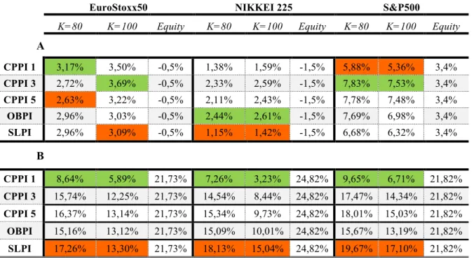
Table 1 compares the latter of the five proposed strategies – CPPI 1, CPPI 3, CPPI 5,
OBPI and SLPI – with both 80% and 100% floor value.
Table A: Annualized Expected Returns (A) and Volatilities (B)
EuroStoxx50 NIKKEI 225 S&P500
K=80 K=100 Equity K=80 K=100 Equity K=80 K=100 Equity
A
CPPI 1 3,17% 3,50% -0,5% 1,38% 1,59% -1,5% 5,88% 5,36% 3,4%
CPPI 3 2,72% 3,69% -0,5% 2,33% 2,59% -1,5% 7,83% 7,53% 3,4%
CPPI 5 2,63% 3,22% -0,5% 2,11% 2,43% -1,5% 7,78% 7,48% 3,4%
OBPI 2,96% 3,03% -0,5% 2,44% 2,61% -1,5% 7,69% 6,98% 3,4%
SLPI 2,96% 3,09% -0,5% 1,15% 1,42% -1,5% 6,68% 6,32% 3,4%
B
CPPI 1 8,64% 5,89% 21,73% 7,26% 3,23% 24,82% 9,65% 6,71% 21,82%
CPPI 3 15,74% 12,25% 21,73% 14,54% 8,44% 24,82% 17,47% 14,34% 21,82%
CPPI 5 16,37% 13,14% 21,73% 15,34% 9,73% 24,82% 18,01% 15,03% 21,82%
OBPI 15,16% 13,12% 21,73% 15,09% 10,01% 24,82% 15,67% 13,19% 21,82%
SLPI 17,26% 13,30% 21,73% 18,13% 15,04% 24,82% 19,67% 17,10% 21,82%
(20)
As presented above, all the strategies can overcome the return associated with the
respective benchmark. For markets that exhibit high negative trend (i.e. NIKKEI 225),
the SLPI strategy is clearly the worst one. This relationship is even more pressing
considering its volatility, which in 83% of cases (on average) makes the strategy reaches
the floor, giving returns equal to 0% and -20% to floors of 100%, and 80%, respectively.
This relationship tends to dissipate when the market returns are less negative (i.e.
EuroStoxx 50), where the CPPI 5 strategy already shows some tendency for returns
below their peers. This is not at all extraneous to their high volatility, making them the
most risky strategy.
Concerning the existent relation between the floor and return, when the markets have a
negative performance and the floor is higher, the strategy also has a higher average return,
demonstrating that in this kind of scenarios, and purely in terms of mean-variance theory,
investors who are focused exclusively in the highest payoffs, must choose higher floors in
order to maximize their profitability. Attending the fact that with lower floors we have
higher exposure to the underlying asset, when the corresponding index has negative
performance ceteris paribus, obviously the strategy with lower floor will have a more
negative expected return. For the U.S. market (i.e. S&P500), with higher positive returns,
all strategies which have lower floors show higher profitability. In these cases, when the
market rises, the lower floors enhance gains in the stock market, since they allow higher
exposure to market bullish tendency. However, and contrary to the expectations, the most
profitable strategy is the CPPI 3, in favour of CPPI 5. From our analysis, this is due to the
high probability of a 5x leverage exposure to the market, which potentiates higher
probabilities of reaching the floor when the market goes down in the beginning of the
these cases the cushion is residual, getting the strategy closer to the barrier along the
investment horizon. However, this evidence lacks scientific confirmation.
5.1.2. Ratio Analysis
As mentioned above, the performance analysis is traditionally based on the
mean-variance analysis. We complete this analysis with some performance measures, such as
the traditional Sharpe Ratio and other measures consistent with Downside Risk: the
Sortino Ratio and the Omega Ratio.
The first one (1), Sharpe Ratio (Sharpe (1994)) can be described as the cost of each unit
of risk, and on the other hand, how much return costs one additional unit of risk. Its value
is given by:
Sharpe Ratio= Rp−Rf
σp
where, Rp is the portfolio return, Rf is the risk-free asset and σp the total risk of each PI
strategy. Despite some disadvantages in terms of consistency with PI strategies (see e.g.
Annaert et al. (2009)) this is a commonly used ratio in finance to rank common
investments between themselves.
The Sortino Ratio measures the excess return over a Minimum Acceptable Return (MAR)
defined by each investor (for theoretical explanation, see e.g. Sortino and Price (1994)).
Although derived from the Sharpe, the Sortino Ratio uses other type of volatility – the
one below MAR – giving us the cost of each unit of “negative” volatility. Its value can be
reached using the following expression.
Sortino Ratio=
(
rp−MAR)
σd ;σd =min"#
(
ri−MAR)
, 0$%2 nt=1
n
∑
The Omega Ratio was developed by Shadwick and Keating (2002), and is a measure of
risk that involves both the likelihood of having a gain associated with an investment in
risky assets, such as the probability of having a loss. The higher the ratio, the better is the
result since the probability of having a loss rather than a gain will be smaller.
All the results for our strategies are presented in Table 2.
Table B: Average Sharpe Ratio (A), Sortino Ratios (B) and Omega Ratios (C).
EuroStoxx50 NIKKEI 225 S&P500
K=80 K=100 Equity K=80 K=100 Equity K=80 K=100 Equity
A
CPPI 1 -0,043 -0,007 -0,19 0,004 0,074 -0,12 0,216 0,232 -0,02
CPPI 3 -0,052 0,012 -0,19 0,067 0,147 -0,12 0,231 0,260 -0,02
CPPI 5 -0,056 -0,024 -0,19 0,050 0,111 -0,12 0,221 0,245 -0,02
OBPI -0,038 -0,039 -0,19 0,072 0,126 -0,12 0,248 0,241 -0,02
SLPI -0,034 -0,034 -0,19 -0,011 0,005 -0,12 0,146 0,147 -0,02
B
CPPI 1 -0,302 -0,048 -1,95 0,413 0,508 -4,67 1,524 1,651 -1,26
CPPI 3 -0,365 0,079 -1,95 0,730 1,000 -4,67 1,603 1,810 -1,26
CPPI 5 -0,381 -0,175 -1,95 0,635 0,952 -4,67 1,524 1,683 -1,26
OBPI -0,373 0,063 -1,95 0,608 0,179 -4,67 1,592 1,768 -1,26
SLPI -0,338 -0,238 -1,95 -1,21 0,023 -4,67 0,324 0,237 -1,26
C
CPPI 1 0,82 0,88 - 0,71 0,77 - 2,01 1,90 -
CPPI 3 0,77 0,79 - 0,66 0,69 - 2,60 2,38 -
CPPI 5 0,67 0,71 - 0,59 0,61 - 2,62 2,35 -
OBPI 0,80 0,86 - 0,66 0,68 - 2,42 2,25 -
SLPI 0,96 0,97 - 0,88 0,91 - 1,93 1,82 -
(23)
In terms of ratio analysis, and considering the basic Sharpe Ratio, the best strategies are
clearly OBPI and CPPI, for the two floor levels. In practice, this means that these are the
strategies that pay better the assumed levels of risk. On the other hand, if we take into
account only the negative returns, the scenario is quite similar. In this case, despite the
relative proximity of the OBPI strategy, CPPI 3 is the one which transversely presents
best positive results. In terms of negative results, SLPI presents the worst ones. This is
due to the high volatility of these instruments, which is not paid for their return.
5.3 Statistical Analysis
Relative Kurtosis and Relative Skewness are two particular ways to define the probability
distribution functions expressed by portfolio insurance terminal values. The Skewness
coefficient is a measure of asymmetry which studies the probability concentrated in the
distribution tails. This allows determining if our probability distribution function has
higher probabilities concentrated far from the mean, consistent with the existence of
outliers – normal distributions have skewness closer to 0. On the other hand, many
researchers suggests that larger skewness makes a protection strategy more appealing (see
Harvey and Siddique (2000) and Port et al. (2008)).
The Kurtosis has the same properties of skewness, but it can tell us more particular things
about the real distribution. A leading example originated from finance can be seen when
performing a distribution function of an index where distribution tends to be leptokurtic –
really peaked with fat tails, which concentrates higher probabilities around the mean but
also presents a higher number of outliers. For normal distributions, its value should be
Table C: Relative Skewness
Table D: Relative Kurtosis
EuroStoxx50 NIKKEI 225 S&P500
K=80 K=100 Equity K=80 K=100 Equity K=80 K=100 Equity
CPPI 1 8,723 9,399 7,43 10,341 11,695 7,95 9,222 10,028 8,46
CPPI 3 16,847 22,926 7,43 28,452 38,147 7,95 15,588 21,615 8,46
CPPI 5 19,103 30,835 7,43 40,602 73,648 7,95 17,906 29,684 8,46
OBPI 89,674 96,130 7,43 81,282 74,590 7,95 49,476 34,672 8,46
SLPI 130,507 97,480 7,43 89,154 78,798 7,95 12,262 24,561 8,46
Concerning relative skewness, it is possible to observe that all strategies present a
behaviour worse that the market. However, the SLPI strategy presents results clearly far
from the market behaviour, for both Kurtosis and Skewness. These results, while
unexpected, are easily explained by the tendency to reach the barrier too soon. From the
moment the portfolio value reaches the lowest barrier strategy, all returns will be positive,
skewing the distribution to the right. On the other hand, if the portfolio´s value reaches
the barrier, all the remaining results will be close to the free-risk interest rate, creating
large fat tails on the distribution, thereby explaining the results for kurtosis.
5.4 Other Measures
To describe the outcomes for each strategy, we performed a descriptive analysis based on
the comparison between equity performance and the portfolio insurance strategies
outcomes. These results are presented in Figures 4 through 6.
EuroStoxx50 NIKKEI 225 S&P500
K=80 K=100 Equity K=80 K=100 Equity K=80 K=100 Equity
CPPI 1 0,135 0,137 0,13 -0,557 -0,575 -0,52 -0,218 -0,215 -0,20
CPPI 3 -0,169 -0,331 0,13 -1,340 -1,595 -0,52 -0,506 -0,673 -0,20
CPPI 5 -0,230 -0,605 0,13 -1,737 -2,613 -0,52 -0,592 -0,946 -0,20
OBPI -0,174 -0,352 0,13 -1,193 -1,023 -0,52 -0,513 -0,692 -0,20
Figure 6: Payoff function for CPPI 3 (A), CPPI 5 (B) and SLPI (C) with floor equals to (1) 80% and (2) 100% (DJ EuroStoxx50).
C2 A2
A1 A2
A1
B2 B1
Figure 7: Payoff function for CPPI 3 (A), CPPI 5 (B) and SLPI (C) with floor equals to (1) 80% and (2) 100% (NIKKEI 225).
B1 B2
C1 C2
A1 A2
Figure 8: Payoff function for CPPI 3 (A), CPPI 5 (B) and SLPI (C) with floor equals to (1) 80% and (2) 100% (NIKKEI 225).
Opposed to many investors opinion, these strategies cannot be described as linear. This
means that it is not only the entry point and the terminal value that matter for the portfolio
performance, but also the portfolio’s movements during the time horizon. This relation is
particularly explicit if we look to the previous diagrams. Other important aspect is the
larger dispersion that tends to exist for CPPI 3 and CPPI 5 (Subfigure A and B of each
Figure) comparing to SLPI (Subfigure C). These results support our previous analysis in
terms of volatility, skewness and kurtosis.
5.5 Stochastic Dominance Analysis
5.5.1 Testing stochastic dominance
For the proposed analysis, we studied the three orders of stochastic dominance (SD) for
all the indexes followed in the previous chapter – EuroStoxx50, NIKKEI225 and
S&P500. To find the stochastic relation between portfolio insurance strategies, we also
define also the two floors suggested before – 80% and 100% - which are commonly used
to study these investments. The set of strategies considered are presented in Tables 9
through 116.
Table E: Stochastic Dominance Test for EuroStoxx50 with a floor at maturity of 80% (FSD: First Order SD; SSD: Second Order SD; TSD: Third Order SD; NSD: No SD)
K=80 K=100
CPPI 1 CPPI 3 CPPI 5 OBPI SLPI CPPI 1 CPPI 3 CPPI 5 OBPI SLPI
CPPI 1 - SSD SSD SSD SSD - SSD SSD NSD SSD CPPI 1
CPPI 3 NSD - SSD NSD SSD NSD - SSD NSD SSD CPPI 3
CPPI 5 NSD NSD - NSD NSD NSD NSD - NSD SSD CPPI 5 OBPI NSD NSD NSD - SSD NSD NSD NSD - SSD OBPI
SLPI NSD NSD NSD NSD - NSD NSD NSD NSD - SLPI
Table F: Stochastic Dominance Test for NIKKEI225 with a floor at maturity of 80% (FSD: First Order SD; SSD: Second Order SD; TSD: Third Order SD; NSD: No SD)
K=80 K=100
CPPI 1 CPPI 3 CPPI 5 OBPI SLPI CPPI 1 CPPI 3 CPPI 5 OBPI SLPI
CPPI 1 - TSD TSD TSD TSD - NSD NSD TSD SSD CPPI 1
CPPI 3 NSD - SSD NSD SSD NSD - SSD NSD SSD CPPI 3
CPPI 5 NSD NSD - NSD SSD NSD NSD - NSD SSD CPPI 5
OBPI NSD NSD NSD - FSD NSD NSD SSD - FSD OBPI
SLPI NSD NSD NSD NSD - NSD NSD NSD NSD - SLPI
Table G: Stochastic Dominance Test for S&P500 with a floor at maturity of 80% (FSD: First Order SD; SSD: Second Order SD; TSD: Third Order SD; NSD: No SD)
Concerning the first SD order, we found six cases where the pattern of dominance exists.
In such cases, where investors prefer more to less (condition of dominance), the strategy
SLPI is clearly the most penalized. However, this strategy is possibly the one that most
suffers from the absence of transaction costs considered in this analysis. Nevertheless,
high levels of volatility tend to make many of the simulations quickly approach the floor
of the strategy continuing on the risk-free rate throughout the time horizon. This
relationship is particularly strong in cases where the floor was set at 100% because the
floor tends to be on a much higher value than for 80%.
On the second and third order of dominance we found similar results. Taking into account
that investors with second order relations of dominance are risk-averse, we concluded
that investors who position themselves in European markets (i.e. EuroStoxx 50) should
choose less aggressive strategies, such as Buy-and-hold strategies (e.g. CPPI 1), which
have higher levels of dominance over the other ones (in this case). The relationship
between dominance and multiple associated with CPPI strategies is also present in the
dominance relationship between the CPPI 3 and 5 for both floors. In these cases, CPPI 3
dominates CPPI 5 in both markets where distributions are clearly skewed to the left (i.e.
EuroStoxx50 and Nikkei 225). This relationship is also true for S&P500, despite its a
clearly upward trend, the CPPI 3 continues with second and third order levels of
stochastic dominance for a floor of 100% and 80% respectively over CPPI 5.
K=80 K=100
CPPI 1 CPPI 3 CPPI 5 OBPI SLPI CPPI 1 CPPI 3 CPPI 5 OBPI SLPI
CPPI 1 - NSD NSD NSD NSD - NSD NSD NSD TSD CPPI 1
CPPI 3 NSD - TSD NSD SSD NSD - SSD NSD FSD CPPI 3
CPPI 5 NSD NSD - NSD FSD NSD NSD - NSD FSD CPPI 5
OBPI NSD NSD - SSD NSD NSD NSD - FSD OBPI
SLPI NSD NSD NSD NSD - NSD NSD NSD NSD - SLPI
Do
mi
n
an
6
Conclusions and further research
The goal of the present study was to provide another insight into the controversy over
Portfolio Insurance strategies and intends to contribute to the decision-making process for
future investors in this type of strategies. The main novelty resides in the use of empirical
distributions and singular methodologies, and the extensive comparison between such
different types of instruments.
First, we found that CPPI 1 outperforms other CPPI strategies with higher multiplier in
terms of stochastic dominance. On the other hand, for all the studied indexes with
negative performance (i.e. NIKKEI 225 and EUROSTOXX 50) CPPI 5 cannot dominate
any of the other strategies (except SLPI). In terms of floor analysis, we found that the
highest floor value implies best downside protection.
These results contradicted some other findings such as those presented by Annaert et al.
(2009) and Zagst and Klaus (2011) that reject any stochastic dominance between
strategies. In our analysis, we found some first order stochastic dominance for all the
strategies over SLPI in a market with bullish tendency. This relation also holds for CPPI
1 and 3 over OBPI (with K=100%). In these cases, ambitious investors will choose CPPI
and OBPI strategies over SLPI (for K=80%) and CPPI 3 and 5 over SLPI (for K=100%).
Our results for CPPI 1 are mainly supported by the research done by Costa and Gaspar
(2012).
However, our analysis has some limitations. For future research we suggest that a better
way to analyze these strategies in a more realistic scenario is to introduce transaction
costs into the analysis and study the inflection point of the multiplier. Some recent studies
also suggest that a conditional multiplier could improve the results of this analysis, and
this could be a good way to continue this research. We also suggest that in order to make
7
References
Ameur, H. and J. Prigent (2006). Portfolio Insurance: determination of a dynamic CPPI
multiple as function of state variables. Working Paper, University of Cergy.
Annaert, J., S. Osselaer and B. Verstraete (2009). Performance evaluation of Portfolio
Insurance strategies using Stochastic Dominance Criteria. Jornal of Banking and Finance
33, 272-280.
Basak, S. (2002). A Comparative Study of Portfolio Insurance. Journal of Economic
Dynamics and Control 26, 1217-1241.
Beach, S. (2007). Semivariance in Asset Allocations: Longer Horizons can Handle
Riskier Holdings. Journal of Financial Planning 20(1), 60-69.
Benninga, S. and M. Blume (1985). On the Optimality of Portfolio Insurance. Journal of
Finance 40, 1341-1352.
Bertrand, P. and J. Prigent (2003). Portfolio Insurance Strategies: a comparison of
standards methods when the volatility of the stock is stochastic. International Journal of
Business 8, 15-31.
Bertrand, P. and J. Prigent (2005). Portfolio Insurance Strategies: OBPI versus CPPI.
Finance 26, 5-32.
Black, F. and R. Jones (1987). Simplifying Portfolio Insurance. The Journal of Portfolio
Black, F. And R. Rouhani (1989). Constant Proportion Portfolio Insurance and the
Synthetic Put Option: a comparison. In F. J. Fabozzi (Ed.), Institutional investor focus on
investment management, Ballinger: Cambridge, 695-708.
Black, F. and A. Perold (1992). Theory of Constant Proportion Portfolio Insurance,
Journal of Portfolio Management, Fall, 48-51.
Black, F. and M. Sholes (1973). The Pricing of Options and Corporate
Liabilities..Journal of Political Economy 81, 637-654.
Bookstabber, R. and J. Langsam (2000). Portfolio Insurance Trading Rules. The Journal
of Futures Markets 8, 15-31.
Brooks, R. and H. Levy (1993). Portfolio Insurance: Does it pay? In: Advancesin Futures
and Options Research, JAI Press.
Campbell, J. and R. Shiller (1998). Valuation Ratios and the Long-Run stock Market
Outlook. Journal of Portfolio Management 20(4), 11-26.
Carlstein, E. (1986). The use of subseries values for estimating the variance of a general
statistics from a stationary sequence. Ann. Statistics 14, 1171-1179.
Cesari, R. and D. Cremonini (2003). Benchmarking, Portfolio Insurance and Technical
Analysis: a Monte Carlo Comparison of dynamic strategies of asset allocation. Journal
of Economic Dynamics and Control 27, 987-1011.
Costa, J. and R. Gaspar (2011). Portfolio Insurance: a comparison of alternative
Efron, B. (1979). Bootstrap methods: another look at the jackknife. Annals of Statistics 7,
1-26.
Fama, E. and K. French (1988). Permanent and Temporary Components of Stock Prices.
Journal of Political Economy 96(2), 246-273.
Garcia, C. and F. Gould (1987). An empirical study of portfolio insurance. Financial
Analysts Journal 43, 44-54.
Graflund, A. (2001). Expected Real Return from Swedish Stocks and Bonds. Working
Paper, University of Lund.
Grossman, S. and J. Villa (1989). Portfolio Insurance in Complete Markets: a note.
Journal of Business 62, 473-76.
Hall, P. (1985). Resampling a Coverage Process. Stochastic Processes and Their
Aplications 20, 231-246.
Hansson, B. and M. Persson (2000). Time Diversification and Estimation Risk. Financial
Analysts Journal 56(5), 55-62.
Künsch, H. (1989). The Jackknife and bootstrap for general stationary observations.
Annals of Statistics 17, 1217-41.
Leland, H. and M. Rubinstein (1976). The Evolution of Portfolio Insurance. In: D.L.
Luskin (Ed.), Portfolio Insurance: a guide of dynamic hedging, New York: Wiley.
Leland, H. and M. Rubinstein (1988). The evolution of portfolio insurance. In Dynamic
Perold, A. and W. Sharpe (1988). Dynamic Strategies for Asset Allocation. Financial
Analysts Journal 44, 16-27.
Perold, A. (1986). Constant Proportion Portfolio Insurance. Working Paper, Harvard
Business School.
Poncet, P. and R. Portait (1997). Assurance de Portefeuille. In: Y. Simon (ed.),
Encyclopédiedês Marchés Financiers, Economica, 140-141.
Prigent, J. and F. Tahar (2005). CPPI with Cushion Insurance. Working Paper, University
of Cergy-Pontoise.
Sanfilippo, G. (2003). Stocks, bonds and investment horizon: a test of time diversification
French market. Quantitative Finance 3, 345-351.
Shadwick W. and C. Keating (2002). A Universal Performance Measure. Journal of
Performance Measure 6(3).
Summers, L. (1986). Does the Stock Market Rationally Reflect Fundamental Values?
Journal of Finance 41(3), 591-601.
Zagst, R. and J. Kraus (2001). Stochastic Dominance of Portfolio Insurance Strategies.
I - Stochastic Dominance
Figure A1: Cumulative distribution function for Eurostoxx 50 with K=80. (A) First order
stochastic dominance; (B) Second order stochastic dominance and (C) Third order stochastic
dominance.
A
B
Figure A2: Cumulative distribution function for Eurostoxx 50 with K=100. (A) First order
stochastic dominance; (B) Second order stochastic dominance and (C) Third order stochastic
dominance.
A
B
Figure A3: Cumulative distribution function for NIKKEI225 with K=80. (A) First order
stochastic dominance; (B) Second order stochastic dominance and (C) Third order stochastic
dominance.
A
B
Figure A4: Cumulative distribution function for NIKKEI225 with K=100. (A) First order
stochastic dominance; (B) Second order stochastic dominance and (C) Third order stochastic
dominance.
A
B
Figure A5: Cumulative distribution function for S&P500 with K=80. (A) First order stochastic
dominance; (B) Second order stochastic dominance and (C) Third order stochastic dominance.
A
B
Figure A6: Cumulative distribution function for S&P500 with K=100. (A) First order stochastic
dominance; (B) Second order stochastic dominance and (C) Third order stochastic dominance.
A
B
III - Other Statistics
Table A1: Probabilities associated with the returns provided by Portfolio Insurance Strategies (EUROSTOXX 50)
Table A2: Probabilities associated with the returns provided by Portfolio Insurance Strategies (NIKKEI 225)
P[ ]>0 P[ ]>
P{ }>0 P{ }>
CPPI 1 (K=80) 3,17% 78,47% 31,58% 2,38% 81,63% 29,53% CPPI 1 (K=100) 3,50% 100% 34,24% 2,95% 100% 32,49% CPPI 3 (K=80) 2,72% 34,39% 23,38% 1,01% 32,66% 20,42% CPPI 3 (K=100) 3,69% 100% 19,02% 1,86% 100% 15,58% CPPI 5 (K=80) 2,63% 32,29% 24,05% 0,88% 30,32% 21,17% CPPI 5 (K=100) 3,22% 100% 20,07% 1,52% 100% 16,74% OBPI (K=80) 2,96% 43,31% 28,46% 2,12% 42,57% 26,07% OBPI (K=100) 3,03% 100% 34,83% 2,51% 100% 33,14% SLPI (K=80) 2,96% 33,47% 25,67% 1,12% 31,63% 22,97% SLPI (K=100) 3,09% 100% 16,82% 1,33% 100% 13,13%
P[ ]>0 P[ ]>
P{ }>0 P{ }>
CPPI 1 (K=80) 1,38% 57,97% 36,33% 1,05% 58,86% 34,81%
Table A3: Probabilities associated with the returns provided by Portfolio Insurance Strategies (S&P500)
P[ ]>0 P[ ]>
P{ }>0 P{ }>
CPPI 1 (K=80) 5,88% 89,75% 53,42% 5,02% 94,17% 53,80%
CPPI 1 (K=100) 5,36% 100% 56,25% 4,77% 100% 56,94%
CPPI 3 (K=80) 7,83% 55,44% 42,92% 5,57% 56,04% 42,13%
CPPI 3 (K=100) 7,53% 100% 36,81% 5,28% 100% 35,34%
CPPI 5 (K=80) 7,78% 52,54% 43,54% 5,50% 52,82% 42,82%
CPPI 5 (K=100) 7,48% 100% 35,59% 5,14% 100% 33,99%
OBPI (K=80) 7,69% 63,52% 48,55% 5,77% 65,02% 48,39%
OBPI (K=100) 6,98% 100% 55,53% 5,54% 100% 56,14%
SLPI (K=80) 6,68% 50,52% 42,36% 4,67% 50,58% 41,51%
SLPI (K=100) 6,32% 100% 31,88% 4,20% 100% 29,87%