Emma del Carmen González González
LAOS characterization of
polymer modified bitumens
Emma del Carmen González González
L A OS c har acter ization of pol
ymer modified bitumens
Universidade do Minho
Master thesis
European Master’s in Engineering Rheology
Work performed under the guidance of
Loic Hilliou, PhD.
Hugo Manuel Ribeiro Dias da Silva, PhD.
Emma del Carmen González González
LAOS characterization of
polymer modified bitumens
Universidade do Minho
Acknowledgements
I would like to thank to all the people who helped me during the development this work.
I want to specially thank to my supervisors PhD. Loic Hilliou and PhD. Hugo Manuel Ribeiro Dias
da Silva who kindly guided me during the research project; their advice and feedback was key for
the completion of this work.
I would like to acknowledge that this master thesis was done in the frame of the project
PLASTICROADS (PTDS/ECM/119179/2010). In this regard I want to thank the researcher of this
project M. Sc. Liliana Costa for the incommensurable help she gave me during all the stages of
the project.
I would like to acknowledge that this Master’s thesis is part of the Erasmus Mundus in Engineering Rheology (EURHEO) Program. In this respect, I am very thankful with the EURHEO consortium
for its academic and financial support through all the Master’s, since my first academic year at
KULeuven, Belgium until the closure of my research project at UMinho, Portugal.
I would like to specially thank to the Civil Engineering department at UMinho for its financial
support, and to its staff namely Eng. Carlos Palha and Eng. Hélder Torres for its academic support
given to this research project, as well as PIEP Institute and Polymers engineering department at
UMinho and its staff for the facilities and equipment used during this project.
Finally, I would like to thank to my family and friends, because thanks to their love and advice I
got the strength to finish this project.
Abstract
In the present work, large amplitude oscillatory shear (LAOS) coupled with Fourier transform
rheology (FTR) were used for the first time to characterize the nonlinear rheology of bituminous
binders, including two polymer modified bitumens (PMB) containing EVA and HDPE.
Additionally, a brief study in the linear regime was done to complete the rheological
characterization along with morphological characterization of PMBs by means of fluorescent
optical micrographs. The comparison between the LAOS-FTR characteristics of samples was done
using a rheological approach (all binders compared at either same phase shift angle δ or same
Deborah number, De) and an experimental approach (all binders compared at same frequency). In
all the approaches, EVA PMB had the lowest nonlinear levels compared to HDPE PMB.
Furthermore differences in the nonlinearity among PMBs, parent 70/100 pen grade bitumen, and
benchmark 35/50 pen grade bitumen were also found. The LAOS-FTR fingerprint of bituminous
binders, though unique, held some similitudes with the reported FTR spectra of multiphase and
polymeric systems. For characterization of asphalt binder in the nonlinear regime, the strength of
LAOS-FTR technique over stress relaxation one was confirmed, not only in terms of the sensitivity
but also in terms of the results interpretation. Furthermore LAOS-FTR was used to analyze time
sweep data with the aim to propose FTR quantifiers as indices to predict fatigue performance.
Keywords: LAOS, Fourier Transform Rheology, nonlinear rheology, bitumen, PMB, fatigue,
Resumo
Neste trabalho utilizou-se pela primeira vez a técnica Large Amplitude Oscillatory Shear (LAOS)
associada à técnica de Fourier Transform Reology (FTR), para caracterizar a reologia não-linear
de ligantes betuminosos, nomeadamente betumes modificados com polímeros (PMBs), sendo estes
polímeros EVA e HDPE. Para além disso realizou-se um breve estudo no regime linear para
completar a caracterização reológica, bem como a caracterização morfológica dos ligantes
modificados com polímeros por meio de micrografias óticas fluorescentes. A comparação entre as
características LAOS-FTR das amostras foi realizada usando uma abordagem reológica (todos os
ligantes foram comparados estando no mesmo ângulo de fase δ ou no mesmo número de Deborah,
De) e uma abordagem experimental (todos os ligantes foram comparados à mesma frequência).
Em todas as abordagens, EVA PMB apresentou níveis mais baixos de não-linearidade quando
comparado com o PEAD PMB. Além disso foram encontradas diferenças na não-linearidade entre
os PMBs, o betume base de penetração 70/100 e o betume usado como referência com penetração
35/50. O comportamento LAOS-FTR característico dos ligantes betuminosos, embora único,
apresentou algumas semelhanças com os espectros FTR de sistemas multifásicos e poliméricos
encontrados na literatura. A superioridade da técnica LAOS-FTR, na caracterização em regime
não linear de ligantes de betuminosos, em comparação com as técnicas de stress relaxation foi
confirmada, não só em termos da sensibilidade, mas também em termos de a interpretação dos
resultados. Além disso LAOS-FTR foi usado para analisar dados de time sweep com o objetivo de
Table of Contents 1. Introduction ... 1 1.1. Motivation ... 1 1.2. Objectives ... 2 1.3. Strategy ... 3 1.4. Outline ... 4 2. Literature review ... 5
2.1. Large amplitude oscillatory shear and Fourier transform rheology ... 5
2.1.1. Fourier Transform concept ... 8
2.1.2. The Discrete Fourier Transform (DFT) ... 10
2.1.3. Fourier transform matters of practicality ... 11
2.1.4. Fourier Transform Rheology ... 14
2.1.5. FTR studies of selected classes of materials ... 21
2.2. Bitumen basics ... 25
2.3. Polymer Modified Bitumen (PMB) ... 29
2.4. Bitumen rheology ... 33
2.4.1. Linear rheology ... 33
2.4.2. Nonlinear rheology ... 35
2.5. Test in binders for performance prediction ... 39
2.6. Morphological characterization of PMB samples ... 40
3. Materials and methods ... 43
3.1. Materials ... 43
3.2. Methods ... 45
4. Linear viscoelasticity of asphalt binders and morphological characterization ... 53
4.2. Stress relaxation in linear regime ... 55
4.3. PMBs morphology (FOM) ... 56
5. Experimental method validation of LAOS-FTR test for binders at room temperature. ... 61
5.1. Linearity range of ARES rheometer ... 61
5.2. Experimental conditions for repeatability of LAOS test of binders at room temperature. . 65
5.2.1. Storage duration ... 66
5.2.2. Torsion bar height ... 67
6. LAOS characterization of asphalt binders ... 71
6.1. LAOS asaf of frequency ... 71
6.2. LAOS at same delta (δ) ... 93
6.2.1. Bitumen grades at δ~ 57° ... 94
6.2.2. PMBs and 35/50 at δ ~ 50° ... 97
6.3. LAOS at same Deborah number (De ~ 0.06) ... 101
7. Stress relaxation test of asphalt binders in NLVE region ... 107
8. LAOS-FTR test to predict fatigue behavior ... 113
9. Results discussion ... 121
9.1. Linear viscoelasticity of asphalt binders and morphological characterization ... 121
9.2. LAOS characterization of asphalt binders ... 124
9.3. Stress relaxation test of asphalt binders in NLVE region ... 129
10. Conclusions ... 133
11. References ... 139
Appendix A. Trigonometric integrals ... 147
Appendix B. Rheology basics ... 149
List of figures
Figure 2-1 Schematic representation of a LAOS test: time (up) and frequency domain (down), adapted from [1]. .... 5
Figure 2-2 Representation of the four canonical behaviors of G’ and G’’ in LAOS tests, from [1] ... 6
Figure 2-3 The four characteristic functions in time domain (from left to right): a sine, a rectangular, a triangular and a saw tooth shaped wave, representing: viscoelastic, strain softening, strain hardening, and shear bands. Adapted from [1]. ... 7
Figure 2-4 Analysis of stress curves in time domain based of curve tilting respect to a pure sinusoidal: stress curves (left) and half cycle comparison with a sinusoidal curve (right). Adapted from [1]. ... 7
Figure 2-5 Lissajous plots: in LVE region (left) and in NLVE region (right). ... 8
Figure 2-6 Representation of a sinusoidal wave in (left) time domain and in (right) frequency domain. ... 9
Figure 2-7 Spectra of a square periodic wave composed of several sinusoidal signals, adapted from [4]. ... 9
Figure 2-8 Representation of aliasing. Adapted from [4]. ... 12
Figure 2-9 Periodic signal (up), integer (middle) and non-integer (down) number of cycles windowed, adapted from [4]. ... 13
Figure 2-10 Representation of a symmetric (left) and a non-symmetric wave (right) along with its FT spectra [1]. . 19
Figure 2-11 I3/I1% at 1 Hz for dispersions of PS-PBA coated with AA and ACM: E base suspension undiluted, E.1 and E.2 are water dilutions of E suspension, and A.1 is dispersion of uncoated particles [14]. ... 22
Figure 2-12 Microstructure of PS and iso-dioctyl phthalate ... 24
Figure 2-13 FTR behavior of entangled PS solutions (linear and branched) in iso-dioctyl phthalate at different weight concentration and at = 2: (left) I3/I1 signal and (right) 3 signal asaf of De [13]. ... 24
Figure 2-14 Nonlinear response of a cis- 1,4 polybutadiene loaded with 0.258 volume fraction of carbon black: (upper curve) total harmonicity, (middle curve) I3/I1%, different than (lower curve) I5/I1%. Adapted from [10]. ... 25
Figure 2-15 Bitumen 35/50 (left) in the liquid state at T>60°C and (right) in the semi-solid state at room temperature. ... 26
Figure 2-16 Colloidal representation of bitumen according to the modified Yen model [25] ... 27
Figure 2-17 Slabs of asphalt mixes: (up) mineral aggregates covered with binder, (down) cross section of a slab. .. 28
Figure 2-18 Representation of the different failures that road pavement undergo: rutting and cracking [27] ... 28
Figure 2-19 Schematic representation of physical distillation ... 31
Figure 2-20 Chemical structure and topology of polyethylene ... 32
Figure 2-21 Chemical structure of poly ethyl-vinyl-acetate (EVA) ... 32
Figure 2-22 Mechanical spectra for a 70/100 pen bitumen from vacuum distillation elastic modulus (G´), loss modulus (G’’), loss tangent (tan ), Tref=0°, adapted from [22]. ... 34
Figure 2-23 Mechanical spectra for a 70/100 bitumen with 7.2% wt. of (radial) SBS elastic modulus (G´), loss modulus (G’’), loss tangent (tan ), Tref=0°, adapted from [22]. ... 34
Figure 2-24 Master curves for (a) 150/200 and (b) 60/700 pen grade bitumen modified with a 50:50 mix of EVA and
LDPE. Tref=25°C. Adapted from [24] ... 35
Figure 2-25 Stress relaxation modulus of a 70/100 pen grade bitumen at 20°C for various strains (left), and after the vertical shift (right) [34] ... 36
Figure 2-26 Stress relaxation modulus of a 200/300 pen grade with 8% wt. EVA at 35°C for various strains [34]. .. 37
Figure 2-27 Stress relaxation modulus of a 70/100 pen grade bitumen with 4% wt LLDPE at various strains [34]. . 37
Figure 2-28 Qualitative shapes of the four proposed stress relaxation types: a) SBS, b) EVA, c) SEBS, d) PE, [22]. ... 38
Figure 2-29 Flow curves of a 200/300 pen grade bitumen at different temperatures from [36]. ... 38
Figure 2-30 Flow curves of the previous 200/300 pen grade bitumen with (left) 4 %wt and (rigth) 8 %wt of EVA from [36]. ... 39
Figure 2-31 Example of a micrography of a sample (SBS PMB) without optical smoothness [42] ... 41
Figure 3-1 Comparison of data analysis between Orchestrator (rheometer) and LabView (external) software. ... 49
Figure 3-2 Stress relaxation data analysis: a) raw data acquired from rheometer, b) data obtained at 98% of target strain, c) raw torque and modulus data acquired at 98% of target strain, d) data acquired above the transducer sensitivity limit, e) same as d) showing saturation of data acquisition at ~ 2 s, f) data clean of experimental pitfalls and used for analysis. ... 50
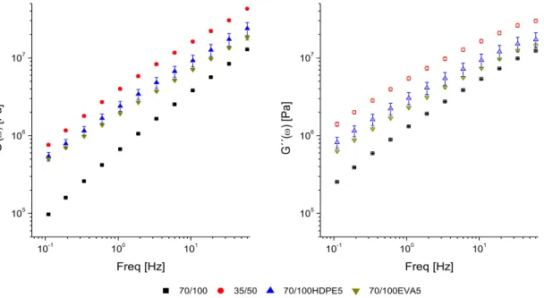
Figure 4-1 Mechanical spectra of bitumen binders at T~ 20°C: G' filled symbols and G'' unfilled symbols. ... 53
Figure 4-2 Phase angle of binders asaf of ω at T~20°C. ... 54
Figure 4-3 Linear stress relaxation modulus of binders at T~20°C. ... 56
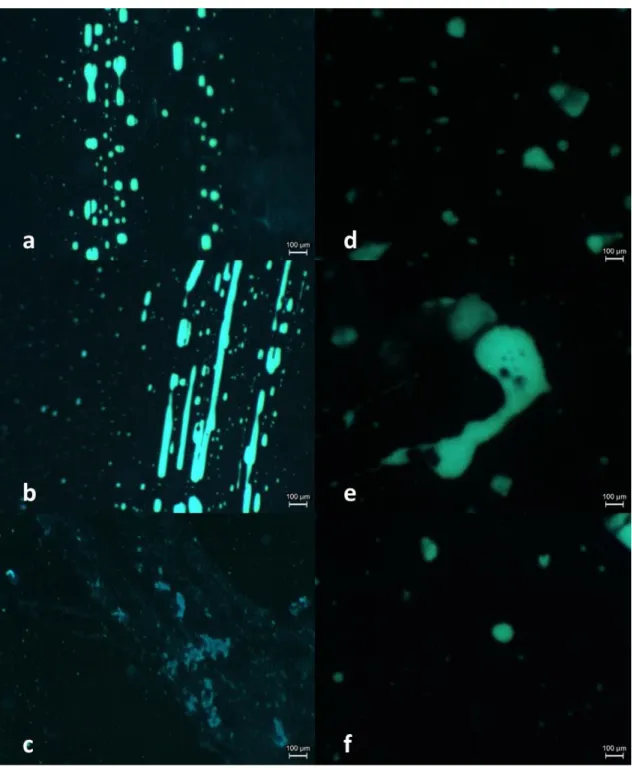
Figure 4-4 FOM micrograph of 70/100EVA5 binder (a,b,c) and 70/100HDPE5 (d,e,f), acquired from the top part of the glass slide.. ... 57
Figure 4-5 FOM micrograph of 70/100EVA5 binder (a,b,c) and 70/100HDPE5 (d,e,f), acquired from the bottom part of the glass slide. ... 59
Figure 5-1 Intervals tested to determine the rheometer linearity range: a) strain, b) torque, and c) motor θ. ... 62
Figure 5-2 Leading nonlinear signal (I3/I1) of the ARES motor at different frequencies measured with PP (filled symbols) and TB (crossed symbols). ... 63
Figure 5-3 Leading nonlinear signal (I3/I1) of the ARES transducer at different frequencies measured with PP (filled symbols) and TB (crossed symbols). ... 64
Figure 5-4 I3/I1% asaf of torque at 5 Hz. For both geometries used it is depicted the transducer I3/I1% and the motor I3/I1% that corresponded to the given torque: PP (filled symbols) and TB (crossed symbols). ... 64
Figure 5-5 Linearity range of ARES rheometer: (left) motor and (right) transducer signal. ... 65
Figure 5-6 Nonlinear response at different bar heights for all the binders. ... 67 Figure 6-1 Pipkin diagram of vs ω for Lissajous curves of 70/100 binder. Additionally in the horizontal axis the
Figure 6-2 Pipkin diagram of vs ω for Lissajous curves of 35/50 binder. Additionally in the horizontal axis the
corresponding De and values are given. ... 73
Figure 6-3 Pipkin diagram of vs ω for Lissajous curves of 70/100HDPE5 binder. Additionally in the horizontal axis the corresponding De and values are given. ... 73
Figure 6-4 Pipkin diagram of vs ω for Lissajous curves of 70/100EVA5 binder. Additionally in the horizontal axis the corresponding De and values are given. ... 74
Figure 6-5 Example of the nonlinear transient response: (left) stress signal decayed over time and tended to leveled off, and (right) the transient was reflected in a halo in the Lissajous curves. Sample 70/100EVA5 at I3/I1=2% ... 75
Figure 6-6 Comparison of odd (left) and even (right) harmonic signals for 35/50 binder at 2Hz. ... 76
Figure 6-7 First odd harmonics asaf of strain for 35/50 binder at 0.7 Hz. ... 76
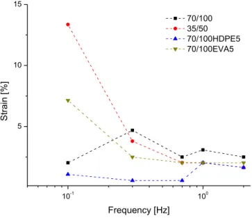
Figure 6-8 Strain for onset of rising of I3/I1 signal, for all binders at all the frequencies tested. ... 77
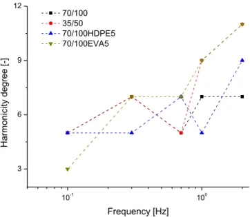
Figure 6-9 Harmonicity degree for all samples tested asaf of frequency. ... 78
Figure 6-10 Example of criteria for valid data in LAOS test: a) raw data, b) fitting of transducer and motor signal, the crossover signaled the valid data without motor noise, which are given in c). ... 79
Figure 6-11 Pipkin diagrams for I3/I1% signal for all binders ... 80
Figure 6-12 I3/I1% data for all samples at all frequencies tested: (unfilled symbols) data free of motor noise, (filled data) data considered for power law, and (solid lines) power law fitting. ... 81
Figure 6-13 Exponent of the power law fitting asaf of frequency for all the binders. ... 83
Figure 6-14 Calculated critical strain for onset of I3/I1 for all samples at different frequencies. ... 84
Figure 6-15 Pipkin diagrams for total harmonicity signal for all binders ... 85
Figure 6-16 Total harmonicity data for all samples at all frequencies tested: (unfilled symbols) data free of motor noise, (filled data) data considered for power law, and (solid lines) power law fitting. ... 86
Figure 6-17 Exponent values of the odd sum power law fitting asaf of frequency for all the binders. ... 87
Figure 6-18 Calculated critical strain for onset of odd sum for all samples at different frequencies ... 88
Figure 6-19 Relative phase angle at different frequencies asaf of strain for all samples. ... 89
Figure 6-20 Strain (left) and stress (right) signals to exemplify the general trend of the stress signal to be tilted to the right. Sample 35/50 at 2 Hz and 25% strain. ... 90
Figure 6-21 Example of the 1st harmonic trend asaf of strain. ... 90
Figure 6-22 Characteristic relative phase angle asaf of frequency for all the binders. ... 91
Figure 6-23 Relative 3rd phase angle asaf of De number for all the binders. ... 92
Figure 6-24 Odd sum fitting parameters re-plotted asaf of delta value (a) pre-exponent and (b) exponent. Characteristic 3rd harmonic phase angle (c) re-plotted asaf of delta. ... 93
Figure 6-25 Relative intensity signals for bitumen grades at ~ 57°: (unfilled symbols) data free of motor noise, (filled data) data considered for power law, and (solid lines) power law fitting. ... 95
Figure 6-26 Phase angle signal asaf of train for binder grades at ~ 57° condition ... 97
Figure 6-27 Relative intensity signals for bitumen grades at ~ 57°: (unfilled symbols) data free of motor noise, (filled data) data considered for power law, and (solid lines) power law fitting. ... 99
Figure 6-28 Relative phase angle signal asaf of strain for binders at ~ 50°. ... 100
Figure 6-29 Relative intensity signals for bitumen grades at De=0.0.6 (unfilled symbols) data free of motor noise, (filled data) data considered for power law, and (solid lines) power law fitting. ... 103
Figure 6-30 Relative phase angle for binders at De ~ 0.06 ... 105
Figure 7-1 Stress relaxation test in nonlinear regime for all binders at T~20°C. ... 107
Figure 7-2 Damping function computed for all the binders at T~20°C, lines are only to guide the eye. ... 108
Figure 7-3 Stress relaxation modulus shifted according to the damping function value for all samples. ... 110
Figure 7-4 Repetition of the stress relaxation test at 0.05% strain for sample 70/100HDPE5 at T~20°C: (left) stress relaxation modulus and torque signals, (right) strain signal. ... 111
Figure 8-1 Time sweeps at same delta and I3/I1=2% for 35/50 and 70/100EVA5 binders. ... 114
Figure 8-2 Time sweeps at same delta and I3/I1=3% for 35/50 binder and PMBs... 115
Figure 8-3 Time sweeps at same delta and I3/I1=4% for PMBs. ... 116
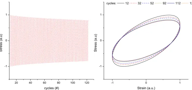
Figure 8-4 I3/I1% signal asaf of cycles number for all binders (log-log representation). ... 117
Figure 9-1 Mechanical spectrum of binder grades: data of 70/100 binder were horizontally shifted by 10Hz to overlap the 35/50 data. ... 122
Figure 9-2 I3/I1 signal for all binders asaf of De at an arbitrary 20.3% strain ... 126
Figure 9-3 Binders I3/I1% response at specific frequencies that shown a bump in the nonlinear signal. ... 128
Figure B-1 Schematic representation of simple shear flow (left), and simple shear deformation (right). ... 149
Figure B-2 Schematic representation of drag and pressure flows. ... 150
Figure B-3 Geometries available to study shear deformation in rotational rheometers, adapted from [58]. ... 150
Figure B-4 Schematic representation of strain controlled and stress controlled rheometers, adapted from [60]. ... 151
Figure B-5 Schematic representation of a stress relaxation experiment: strain imposed (left), canonical responses per material type (right). ... 154
Figure B-6 Schematic representation of a Maxwell model mechanical spectra. ... 158
Figure C-1 Lissajous curves for binder samples at ~ 57° ... 159
Figure C-2 Lissajous curves for binder samples at ~ 50° ... 160
List of tables
Table 2-1 Fourier analysis techniques... 10
Table 2-2 Bitumen composition and basic characteristics according to the SARA fractions [22] ... 26
Table 3-1 Polymer transition temperatures ... 43
Table 3-2 PMBs specs ... 44
Table 3-3 Clamping force used to lock the samples in the rectangular geometry ... 46
Table 3-4 Data acquisition details for FFT computation ... 47
Table 4-1 Crossover frequency of the different binders at T~ 20°C. ... 55
Table 5-1 Experimental conditions studied to determine the linearity range of the ARES rheometer. ... 62
Table 5-2 Statistical analysis of linear and nonlinear parameters asaf of the days in the freezer ... 66
Table 5-3 Frequencies used in the LAOS tests for bar height determination... 67
Table 5-4 Relative standard deviation associated to the experimental repeatability ... 68
Table 5-5 Repeatability results for power law fitting of ATBs at 2.5 cm height ... 69
Table 6-1 Experimental conditions for LAOS tests at different frequencies ... 71
Table 6-2 Power law fitting results of I3/I1 signal for all binders at different frequencies ... 82
Table 6-3 Power law fitting results of odd sum signal for all binders at different frequencies ... 87
Table 6-4 Characteristic relative phase angle of the 3rd harmonic for all the samples at different frequencies. ... 89
Table 6-5 Experimental conditions for ~ 57° ... 94
Table 6-6 Harmonicity degree found in both bitumen grades at ~ 57°. ... 94
Table 6-7 Power law fitting results of nonlinear signals for binder grades at ~ 57°. ... 94
Table 6-8 Limit condition for nonlinear signal used to compute the critical strains, as well as the sample from which the limiting value was obtained. ... 96
Table 6-9 Critical strains for nonlinear signals at ~ 57° condition ... 96
Table 6-10 Characteristic relative phase angle data for different harmonics of bitumen grades at ~ 57°. ... 97
Table 6-11 Experimental conditions for ~ 50° ... 97
Table 6-12 Harmonicity degree for binders at ~ 50°... 98
Table 6-13 Power law fitting results of nonlinear signals for binder grades at ~ 50°. ... 98
Table 6-14 Critical strains for nonlinear signals at ~ 50° condition ... 100
Table 6-15 Characteristic relative phase angle data for different harmonics of bitumen grades at ~ 57°. ... 101
Table 6-16 Experimental conditions for De ~ 0.06 ... 102
Table 6-17 Harmonicity degree for binders at De ~ 0.06 ... 102
Table 6-19 Critical strains for nonlinear signals at De=0.06 condition ... 104
Table 6-20 Relative phase angle for binders at De ~ 0.06 ... 105
Table 7-1 Damping function sigmoidal fitting and time validity. ... 109
Table 8-1 Experimental conditions for time sweep tests in NLVE regime. ... 113
Table 8-2 Results summary of time sweep tests ... 118
Table 9-1 Computed 533 −5 to support the existence of a relationship between relative phase angles of binders ... 127
Table 9-2 Frequencies at which binders shown a bump in the I3/I1% signal ... 127
Nomenclature, abbreviations and acronyms
Nomenclature
𝐶𝑎 Capillary number [-]
𝐷𝑒 Deborah number [-]
𝐺 shear modulus [Pa]
𝐺(𝑡) linear stress relaxation modulus [Pa]
𝐺(𝑡, 𝛾) nonlinear stress relaxation modulus [Pa]
𝐺′ elastic or real modulus – real 1st harmonic intensity [Pa]
𝐺′′ viscous or loss or imaginary modulus – complex 1st harmonic intensity [Pa]
𝐺∗ complex shear modulus [Pa]
𝑖 imaginary number √−1
𝐼𝑛 nth harmonic intensity [Pa]
𝐼𝑛/𝐼1 nth harmonic relative intensity [-]
𝑘 kth harmonic idem as 𝑛
𝑛 nth harmonic
N number of data points for FFT
𝑝 viscosity ratio [-]
𝑡 time [s]
𝑡𝑑𝑤 dwelling time [s]
𝑡𝑎𝑞 acquisition time [s]
𝑇 temperature [°C]
𝑇𝑅&𝐵 ring and ball temperature [°C]
𝑋𝑑(𝑘𝜔0) kth FT coefficient
𝛾 shear strain [-]
𝛾̇ shear strain rate [1/s]
𝛾𝑐 critical strain and critical strain in total harmonicity signal [-]
𝛾𝑐−𝑛 critical strain in nth harmonic signal[-]
𝛤 interfacial tension [N/m]
𝛿 loss angle, phase shift or phase lag of stress signal respect to strain signal [°]
𝜂 non-Newtonian shear viscosity[Pa.s]
𝜂𝑚 matrix viscosity
𝜂𝑑 dispersed phase viscosity
𝜆 (characteristic) relaxation time [s]
𝜇 Newtonian viscosity [Pa.s]
𝜎 shear stress [Pa]
𝜎̇ time derivative of shear stress [Pa/s]
𝑛 phase angle of nth harmonic respect to a cosine curve that starts a 𝑡 = 0 𝑠 [°]
𝑛− 𝑛1 relative phase angle of nth harmonic respect to the signal of the fundamental [°]
n abbreviation for 𝑛− 𝑛1
𝜔 frequency [Hz]
𝜔0 fundamental frequency [Hz]
𝜔𝑐 crossover frequency [Hz]
Abbreviations and acronyms
AA Acrylic acid
ACM Acrylamide
ARP asphalt rich phase
asaf as a function of
ATB asphalt torsion bar
DFT discrete Fourier transform
EVA Poly ethyl-vinyl-acetate
FFT fast Fourier transform
FOM fluorescent optical microscopy
FT Fourier transform
FTR Fourier transform rheology
HDPE High density polyethylene
Im imaginary part of a complex number
LAOS large amplitude oscillatory shear
LVE linear viscoelasticity or linear viscoelastic
MAOS medium amplitude oscillatory shear
n/a not available or not applicable
NLVE nonlinear viscoelasticity or nonlinear viscoelastic
OM order of magnitude
PBA polybutylacrylate
PDMS polydimethylsiloxane
PMB polymer modified bitumen
PP parallel plates
PS polystyrene
PRP polymer rich phase
Re real part of a complex number
SAOS small amplitude oscillatory shear
STB steel torsion bar
TB torsion bar
1. Introduction
1.1. Motivation
The study of bitumen is of crucial importance for the production of high performance asphalt roads. This primary idea is justified by the fact that the mechanical properties and performance of the asphalt mixes are clearly influenced by the bitumen, because it is the only deformable component and it conforms the continuous matrix. Furthermore, current traffic loads and economically sustainable trends demand long service life paving roads. In this regard, service life in paving roads is determined by the tendency of the asphalt mix to undergo failures (rutting, fatigue cracking, and thermal cracking) as a consequence of the mechanical history at which it is subjected. In order to increase the service life of road pavements by delaying the emergence of these failures, conventional pen grade bitumens have been modified by the addition of polymers. This process results in polymer modified bitumens (PMBs), which are expected to have improved mechanical properties in comparison with those of the conventional pen grade bitumens they will replace: reflected in asphalt mixes with a longer service life.
Considering above, it can be inferred that characterization of the mechanical properties of binders is of great help in the design of better paving roads. Since a binder is a viscoelastic material, its mechanical properties can be studied by means of rheology. In terms of rheology, microstructure is studied in the linear viscoelastic (LVE) region and microstructural changes due to mechanical fields are studied in the non-linear viscoelastic (NLVE) region.
Linear rheological characterization of binders has been done mainly by means of small amplitude oscillatory shear tests (SAOS), and there is ample information regarding it. In SAOS test the microstructure of the system is preserved due to the low deformations applied. However, SAOS can have limited resolution to distinguish among complex materials with similar microstructure. In fact, linear characterization of asphalt binders has been proven to be unsuccessful in differentiating and predicting performance of PMBs. Furthermore, in service life asphalt is subjected to deformations outside the LVE region. Therefore the LVE characterization is a good starting point to study asphalt binders, but it will lack predictability towards service life performance.
Nonlinear rheological characterization of binders has only recently been reported in more detail. In NLVE characterization the microstructure is changed due to the high deformations applied: it can be more sensitive to small microstructural differences. Furthermore since the deformations applied are large, tests in the nonlinear regime can have a better potential to predict service life performance, as it better simulates limiting service conditions. Non-linear characterization of binders can be done by means of stress relaxation, steady shear flow, creep, and LAOS tests. In current open literature, there is available information for the first two types of tests. Nevertheless, its interpretation for proper ranking and differentiation between bitumens and PMBs has been proven to be difficult, and in most of the cases at most a qualitative differentiation between binders has been done. On the other hand, LAOS test coupled with Fourier transform rheology can yield specific quantifiers of the non-linear behavior of asphalt binders, by means of which a better characterization of bituminous binders could be done.
It is worth to mention that rheological information of binders close to room temperature (20°C – 25°C) is scarce or even null for some rheological tests. Contradictory, room temperature is roughly the mean for service temperature of paving roads in several countries. Furthermore, the reported tests performed around room temperature were done in shearing geometries (parallel plates and cone and plate), which are not suitable for the study of asphalt at room temperature (semisolid material), this could have induced experimental pitfalls and therefore a misinterpretation of the reported results.
Therefore, characterization of asphalt binders at room temperature using a suitable geometry by means of LAOS tests and FTR could provide a better quantitative characterization of the NLVE behavior of asphalt binders. The outputs of this characterization could be potentially more useful not only to differentiate between binders with similar microstructure, but also to give an insight of the service life performance.
1.2. Objectives
The main goal of the present work was to contribute to the bitumen and PMBs rheological
characterization under large deformation at service temperature (𝑇~20°𝐶) by means of
The specific goals were:
To use a torsional bar geometry as an alternative to allow for the NLVE study of binders at room temperature (𝑇~20°𝐶).
To design and validate a LAOS-FTR experimental protocol to study the NLVE behavior of bitumen and PMB.
To establish whether LAOS-FTR outputs can efficiently distinguish between the nonlinear rheological behavior of different bitumens and PMBs.
To relate LAOS-FTR outputs with morphological properties.
To compare LAOS-FTR data with stress relax data for characterization of NLVE behavior of binders.
To explore the possibility to apply LAOS-FTR as a fast technique to characterize binders’ fatigue behavior.
Above studies were done using two binder grades: 70/100 pen grade (parent bitumen) and 35/50 pen grade (benchmark bitumen), and two thermoplastic polymer modified bitumens: 70/100 pen grade with 5% wt. of recycled EVA copolymer (70/100EVA5), and 70/100 pen grade with 5% wt. of recycled HDPE copolymer (70/100HDPE5).
Finally in view that LAOS test is currently used to predict fatigue performance in binders, it seemed logical to expand this technique in terms of Fourier transform rheology quantifiers to clarify whether FTR could have some potential for data analysis.
1.3. Strategy
To start a brief characterization of the binders in the linear regime (SAOS and stress relaxation) was first performed. This in view that linear properties are the set point from which nonlinear properties depart and that linear & nonlinear rheology study different aspects of the material. This first characterization was also complemented with morphological studies of PMBs by means of fluorescent optical microscopy (FOM).
Then to avoid experimental pitfalls prior to start the LAOS-FTR characterization, the determination of the linearity range of the rheometer was done and the experimental conditions to obtain repeatable LAOS-FTR experiments in binders were set.
After the baseline, the playground, and the experimental conditions were established, the LAOS-FTR characterization of the mentioned bituminous binders was done. The LAOS-LAOS-FTR characterization was done in amplitude sweep tests, which were performed using an experimental approach (all binders compared at same frequency) and a rheological approach (all binders compared at either same phase shift angle δ or same Deborah number, De). This was done to compare both approaches in order to select which could have a better potential for binders characterization. The binders FTR fingerprint obtained was compared with literature data of specific materials classes (emulsions, suspensions, polymers, etc.) to link morphological similitudes.
Then considering that time sweep tests are currently used to predict fatigue behavior in binders and that LAOS-FTR is a very sensitive technique, time sweep test data in the nonlinear regime were analyzed by FTR.
1.4. Outline
The present work will begin with a literature review given in chapter 2, and then a description of the materials and methods used in chapter 3. Afterward, in chapter 4 the LVE characterization of asphalt binders is given along with the FOM study. The determination of the rheometer linearity range and the methodology to obtain repeatability in LAOS test are presented in chapter 5. The NLVE characterization of asphalt binders by LAOS-FTR is presented in chapter 6. Subsequently, the nonlinear stress relaxation tests are given in chapter 7. The implementation of LAOS-FTR to predict fatigue behavior is introduced in chapter 8. The discussion of the results is provided in chapter 9 and the conclusions and further work are drawn in chapter 10.
2. Literature review
2.1. Large amplitude oscillatory shear and Fourier transform rheology
Large amplitude oscillatory shear (LAOS) is a useful test for nonlinear characterization of complex fluids, because strain amplitude and frequency are decoupled, and it does not involve any sudden jump in stress or strain: it is a relatively easy flow to generate [1, 2].
As expected, in the NLVE regime the rheological functions (𝐺’, 𝐺’’, 𝐺∗, 𝛿) depend not only of the
frequency (time), but also of the deformation amplitude. This is reflected in the fact that the stress (or strain) output is no longer a pure sinusoidal signal [3], though the LAOS strain (or stress) input is ideally a pure sinusoidal. In fact, the output signal is a sum of several sinusoidal waves: even if not sinusoidal the output stress is yet periodic.
The most common LAOS test mode is a strain sweep, illustrated in Figure 2-1 on which it is clear that the moduli depend on strain and that the stress output is no longer a pure sinusoidal curve. Still, any dynamic test carried out outside the LVE region can be named LAOS test [1], e.g. frequency sweep test at a strain amplitude in the NLVE region.
In LAOS strain sweep test, there were reported four canonical responses for 𝐺’ and 𝐺’’ which are shown in Figure 2-2: type I, strain thinning (𝐺’ and 𝐺’’ decreasing); type II, strain hardening (𝐺’ and 𝐺’’ increasing); type III, weak strain overshoot (𝐺’ decreasing, 𝐺’’ increasing followed by decreasing); type IV, strong strain overshoot (𝐺’ and 𝐺’’ increasing followed by decreasing). Each type has been related to specific types of materials. Type I is the most common behavior in polymer solutions and melts. Since asphalt has shown similar rheology to a low molecular weight polymer this behavior was the one expected.
Figure 2-2 Representation of the four canonical behaviors of G’ and G’’ in LAOS tests, from [1]
Considering the above, for a strain sweep test in LAOS (which in the following will be referred only as LAOS test) the frequency at which the test is performed is also important (because the material is viscoelastic). The frequency to perform the test can be chosen to be either below, at, or above the crossover point between 𝐺’ and 𝐺’’. To have a more complete analysis LAOS tests can be carried out at several frequencies to evidence the viscoelastic nonlinear response. Furthermore, some other modes of comparison are used, e.g. test the samples at the same value of tan 𝛿 i.e. test samples mechanically equivalent, test the samples at the De number i.e. test samples at same relaxation state.
Since in LAOS the response of the material becomes more complex as compared to SAOS, the results analysis has also to be done in a different way. In general LAOS test analysis can be done either in time, or in deformation, or in frequency domain.
Data analysis in the time domain is done by means of stress curve shapes. Reported stress curve analysis are based on the departure from a pure sinusoidal shape, and their canonical forms are shown in Figure 2-3, while the tilting degree analysis is shown in Figure 2-4, among others [1].
Figure 2-3 The four characteristic functions in time domain (from left to right): a sine, a rectangular, a triangular and a saw tooth shaped wave, representing: viscoelastic, strain softening, strain hardening, and shear bands.
Adapted from [1].
Figure 2-4 Analysis of stress curves in time domain based of curve tilting respect to a pure sinusoidal: stress curves (left) and half cycle comparison with a sinusoidal curve (right). Adapted from [1].
However one of the most used data analysis is Lissajous plots which correspond to the deformation domain. Lissajous plots are closed loop plots of 𝜎 vs 𝛾 (or 𝜎 vs 𝛾̇) which canonical forms for elastic, viscous, and viscoelastic materials in the LVE region are shown in Figure 2-5. In the nonlinear regime, the shape of the canonical forms is deformed, shown in Figure 2-5 as well.
Analysis of Lissajous plots can be done by visual inspection of the curves deformation (qualitative), and by quantification of the deformation by means of integration of the curve area (quantitative). The former analysis is a good method for rapid qualitative evaluation.
Figure 2-5 Lissajous plots: in LVE region (left) and in NLVE region (right).
Even though these plots do not yield any information regarding microstructure, they demonstrate how nonlinearity can affect the output signal of a VE material. Despite the fact that these visual analysis is useful, quantitative methods are also needed to fully analyze the nonlinear response of the material. In this regard Fourier Transform Rheology (FTR) is the preferred quantitative method to analyze stress curves in the nonlinear region, and it is done in the frequency domain. Fourier transformation is described in the next section.
2.1.1. Fourier Transform concept
Fourier analysis techniques consist in transforming a signal in the time domain to a signal in the frequency domain. The frequency domain representation can give a different insight about the time signal. Hence time and frequency representation describe the same signal, but from a different point of view [4].
To illustrate this time-frequency correspondence, a sinusoidal wave is shown in Figure 2-6, and in the frequency domain this signal is represented in magnitude and phase charts, also shown in Figure 2-6.
In the magnitude plane the amplitude of the sinusoidal wave is given along with the frequency at which each cycle occurs. In the phase plane, the phase delay respect to time equal to zero is given along with the frequency at which each cycle occurs. With this data from the frequency domain (frequency, amplitude and phase angle) the wave can be reconstructed in the time domain [4].
0.0 0.2 0.4 0.6 0.8 1.0 -2 0 2 0 1 2 0.0 0.5 1.0 1.5 2.0 0 1 2 -90 -60 -30 0 30 60 90 2s in(t) [-] Time [s] A mp litu de [-] Freq [Hz] ph as e [°] Freq [Hz]
Figure 2-6 Representation of a sinusoidal wave in (left) time domain and in (right) frequency domain.
Fourier analysis is spectrum analysis, and different wave shapes have different spectra. More complicated periodic functions will be composed of the sum of several waves. In the spectra each wave (or spectral component) is represented by a single line or impulse which are located in the frequency axis at integer multiples of the fundamental frequency. Each of these Fourier terms is referred as a harmonic. Each harmonic will have a spectral line in the magnitude and in the phase diagram, shown in Figure 2-7.
Figure 2-7 Spectra of a square periodic wave composed of several sinusoidal signals, adapted from [4].
Fourier analysis is intended for several types of function (continuous, discrete, periodic, and non-periodic). Therefore, in Fourier analysis there are three types of transformations: Fourier series, Fourier Integral, and discrete Fourier transform. The main characteristics and differences between these techniques are given in Table 2-.
In the case of the Fourier series and the Fourier integral, the function to be transformed must be described by a mathematic expression. In other words, if the function cannot be set to an equation,
then the classic Fourier techniques cannot be applied. This is impractical for real waves acquired in an experiment (e.g. in oscillatory shear). On the other hand, considering that a real wave is continuous then by definition is not suitable for Discrete Fourier Transform (DFT) analysis. However, a real wave can be sampled in a set of discrete points, and then the DFT can be used to analyze the signal in the frequency domain.
Table 2-1 Fourier analysis techniques
Fourier technique
Transformation pairs Function type in
tdomain Function type in ωdomain Fourier series 𝑥(𝑡) = 𝑎0+ ∑(𝑎𝑛cos 𝑛𝜔0𝑡 + 𝑏𝑛sin 𝑛𝜔0𝑡) ∞ 𝑛=1 𝑎0= 1 𝑇∫ 𝑥(𝑡)𝑑𝑡 𝑇 0 𝑎𝑛(𝑛𝜔0) = 2 𝑇∫ 𝑥(𝑡) cos 𝑛𝜔0𝑡 𝑑𝑡 𝑇 0 𝑏𝑛(𝑛𝜔0) =2 𝑇∫ 𝑥(𝑡) sin 𝑛𝜔0𝑡 𝑑𝑡 𝑇 0 continuous periodic function frequency charts (magnitude and phase) at specific discrete frequencies Fourier transform (integral) 𝑋(𝜔) = ∫+∞𝑥(𝑡)𝑒−𝑖2𝜋𝜔𝑡𝑑𝑡 −∞ 𝑥(𝑡) = ∫+∞𝑋(𝜔)𝑒𝑖2𝜋𝜔𝑡𝑑𝜔 −∞ continuous non periodic function continuous spectra respect to ω Discrete Fourier Transform (DFT) 𝑋𝑑(𝑘𝜔0) = 𝑡𝑑𝑤∑ 𝑥(𝑛𝑡𝑑𝑤)𝑒−𝑖2𝜋𝑘𝜔0𝑛𝑡𝑑𝑤 𝑁−1 𝑛=0 𝑥(𝑛𝑡𝑑𝑤) = 𝜔0∑ 𝑋𝑑(𝑘𝜔0) 𝑁−1 𝑘=0 𝑒𝑖2𝜋𝑘𝜔0𝑛𝑡𝑑𝑤
discrete sets of data points evenly spaced on time during a finite period of time frequency charts (magnitude and phase) at specific discrete frequencies
2.1.2. The Discrete Fourier Transform (DFT)
The DFT transformation pairs are given on Table 2-1. An alternative representation of above equations can be yielded by means of the Euler’s equation
in terms of cos and sin series, where the coefficients for the cos series give the real part coefficients and the coefficients for the sin series give the imaginary part coefficients. For the DFT
𝑋𝑑(𝑘𝜔0) = 𝑅𝑒(𝑘𝜔0) + 𝑖 𝐼𝑚(𝑘𝜔0)
( 2.1.2-2 )
and considering that any complex pair can be represented in a vectorial form (Argand diagram). Above result can be further expressed as
|𝑋𝑑(𝑘𝜔0)| = √𝑅𝑒(𝑘𝜔0)2+ 𝐼𝑚(𝑘𝜔 0)2
tan =𝐼𝑚(𝑘𝜔0) 𝑅𝑒(𝑘𝜔0)
( 2.1.2-3 )
which yields the harmonic magnitude and phase angle.
Therefore any data in the frequency domain can be described either by real and imaginary (𝐺’ and 𝐺’’) or by magnitude and phase (𝐺∗ and 𝛿) coefficients.
By using above expressions, it is straightforward to compute the DFT for any string of waveform samples. The values of 𝑥(𝑛) are taken directly from the experimental data. Nevertheless the classical DFT algorithm is lengthy and not easy to implement. Because of this, nowadays the so called Fast Fourier transform (FFT) algorithm is used. The FFT algorithm is a fair approximation of the strict DFT one that is capable to yield the same harmonic coefficients in shorter time [4].
2.1.3. Fourier transform matters of practicality
Data acquisition and analysis
Windowing and sampling.
To be analyzed in FFT, a wave has to be windowed and sampled. Windowing is the delimitation of the time period over which the signal analysis will be done. Sampling is the decomposition of the continuous wave in discrete evenly spaced data points. In practice, windowing and sampling is done by an analog to digital converter (ADC) [4].
Signal averaging.
Time-domain noise transforms to frequency-domain noise. In the case that the noise is random, it will have a zero mean. Therefore signal averaging will eliminate the noise and lead to sharper signals, and this is done by analyzing several cycles of the same response. For truly mean-zero noise, the improvement in signal-to-noise ratio for M cycles acquired is √𝑀 [4, 5].
Aliasing.
Aliasing is the representation of a high-frequency component by a lower frequency component, shown in Figure 2-8.
Figure 2-8 Representation of aliasing. Adapted from [4].
To explain aliasing time-frequency relationship of the sampled data points will be introduced. Each data point in time is acquired at a fixed time increment 𝑡𝑑𝑤 or dwellingtime over a total time 𝑡𝑎𝑞 or acquisition time
𝑡𝑎𝑞 = 𝑁𝑡𝑑𝑤
( 2.1.3-1 )
Hence, from 𝑁 real data points by means of FFT a discrete spectrum of 𝑁 complex points is generated. Time and frequency hold a reciprocal relationship. Therefore, the spectral width or maximum frequency is given by
𝜔𝑚𝑎𝑥 =
1
∆𝜔 = 1
𝑡𝑎𝑞 ( 2.1.3-3 )
The Nyquist theorem governs the proper sampling: it states that the sampling rate has to be at least twice the maximum frequency contained in the function to be analyzed [4].
1 𝑡𝑑𝑤
= 2𝜔𝑚𝑎𝑥
( 2.1.3-4 )
In other words, there must be at least two points per cycle for any frequency component contained in the wave. If there are less points then aliasing occurs. Therefore, equation ( 2.1.3-2 ) is correct for
the reciprocal relationship of time and frequency, but due to the Nyquist theorem, equation ( 2.1.3-4 ) is the one that defines the real spectral width.
In real world aliasing is unavoidable, the better is to set the Nyquist frequency at a value high enough so that the signal of the highest frequency component falls beyond the noise. Therefore, in any experiment one should first estimate the maximum possible harmonic contribution (of the maximum harmonic that one wishes to acquire) and adjust the sampling rate accordingly [5].
The major issue with aliasing is that sometimes the high frequency components that are aliased can be erroneously added to low frequency signals, and this will mislead the results [4].
Leakage.
The FFT assumes periodicity in all cases, i.e. the windowed signal will be repeated all over again (shown in Figure 2-9).
Figure 2-9 Periodic signal (up), integer (middle) and non-integer (down) number of cycles windowed, adapted from [4].
In the case where a non-integer number of cycles occur in the window, leakage will smear the frequency-domain information: error will be introduced.
Rheometer equipment
To perform FTR of LAOS data strain controlled rheometers are preferred in order to have a more monochromatic excitation [1]. By supplying a “monochromatic” strain, it is possible to conclude that any stress output at frequencies other than the fundamental is associated with nonlinearities in the system response. To ensure this, a FFT of the motor signal can be done to determine the linear operational range of the motor. In this frame, the transducer linear range has also to be determined [6]. The rheometer used for FTR has to be modified to allow the collection of the raw data signal from motor and transducer by an ADC card [1]. This data can be analyzed with a FFT in many commercial software (Matlab, Mathematica, LabView, etc).
2.1.4. Fourier Transform Rheology
Fourier Transform Rheology (FTR) is the analysis in the frequency domain of a periodic signal coming from oscillatory experiments. In FTR a discrete, complex, half sided FT is commonly used. It is discrete because the DFT technique with a FFT algorithm is used. It is complex because the FT is inherently complex, but also to make the difference that neither only sine nor cosine FT are used. It is half sided because only the positive axis of the frequency is analyzed.
In an oscillatory experiment a sinusoidal strain excitation is used
𝛾(𝑡) = 𝛾0cos(𝜔𝑡)
( 2.1.4-1 )
whose FT is given by the Fourier series
𝐶𝑛(𝑛𝜔0) = 2 𝑇∫ 𝑥(𝑡) 𝑇 0 𝑒−𝑖𝑛𝜔𝑡𝑑𝑡 ( 2.1.4-2 )
Substituting eq. ( 2.1.4-1 ) in eq. ( 2.1.4-2 )
𝐶𝑛(𝜔0) = 2 𝑇∫ 𝛾0cos(𝜔0𝑡) 𝑇 0 𝑒−𝑖𝑛𝜔0𝑡𝑑𝑡 ( 2.1.4-3 )
and by means of Euler’s equation ( 2.1.2-1 ) 𝐶𝑛(𝑛𝜔0) =2 𝑇[∫ 𝛾0cos(𝜔0𝑡) 𝑇 0 cos(𝑛𝜔0𝑡) 𝑑𝑡 − 𝑖 ∫ 𝛾0cos(𝜔0𝑡) 𝑇 0 sin(𝑛𝜔0𝑡) 𝑑𝑡] ( 2.1.4-4 )
Considering the properties of sine and cosine integrals given in Appendix A, only for 𝑛 = 1 above integral is different than zero. Thus equation ( 2.1.4-4 ) is further simplified to
𝐶1(𝜔0) = 𝛾0
( 2.1.4-5 )
whose magnitude and phase angle are computed according to eq. ( 2.1.2-3 ), and given by
|𝐶1(𝜔0)| = 𝛾0
tan= 0
𝛾0
= 0 → 𝛿 = 0° ( 2.1.4-6 )
which is the FT of a cosine strain wave.
In the LVE region, the stress output is given by
𝜎(𝑡) = 𝜎0cos(𝜔0𝑡 + 𝛿)
( 2.1.4-7 )
According to above procedure the FT is given by
or 𝐶𝑛(𝑛𝜔0) = 2 𝑇∫ 𝜎0cos(𝜔0𝑡 + 𝛿) 𝑇 0 𝑒−𝑖𝑛𝜔0𝑡𝑑𝑡 𝐶𝑛(𝑛𝜔0) =2 𝑇[∫ 𝜎0cos(𝜔0𝑡) cos(𝛿) 𝑇 0 𝑒−𝑖𝑛𝜔0𝑡𝑑𝑡 − ∫ 𝜎 0sin(𝜔0𝑡) sin(𝛿) 𝑇 0 𝑒−𝑖𝑛𝜔0𝑡𝑑𝑡 ] ( 2.1.4-8 )
By means of Euler’s equation ( 2.1.2-1 )
𝐶𝑛(𝑛𝜔0) =
2
𝑇[∫ 𝜎0cos(𝜔0𝑡) cos(𝛿)
𝑇 0
cos(𝑛𝜔0𝑡) 𝑑𝑡 − 𝑖 ∫ 𝜎0cos(𝜔0𝑡) cos(𝛿) 𝑇
0
sin(𝑛𝜔0𝑡) 𝑑𝑡
− ∫ 𝜎0sin(𝜔0𝑡) sin(𝛿) cos(𝑛𝜔0𝑡) 𝑇
0
𝑑𝑡 + 𝑖 ∫ 𝜎0sin(𝜔0𝑡) sin(𝛿) sin(𝑛𝜔0𝑡) 𝑇
0
𝑑𝑡]
Considering the integrals in Appendix A, above equation is different than zero only for 𝑛 = 1: 𝐶1(𝜔0) = 2 𝑇[∫ 𝜎0cos(𝜔0𝑡) cos(𝛿) 𝑇 0
cos(𝜔0𝑡) 𝑑𝑡 + 𝑖 ∫ 𝜎0sin(𝜔0𝑡) sin(𝛿) sin(𝑛𝜔0𝑡) 𝑇
0
𝑑𝑡]
or 𝐶1(𝜔0) = [𝜎0cos(𝛿) + 𝑖 𝜎0sin(𝛿)] ( 2.1.4-10 )
whose magnitude and phase lag are given by
|𝐶1(𝜔0)| = 𝜎0
( 2.1.4-11 )
tan(𝛿) = sin(𝛿)
cos(𝛿) ( 2.1.4-12 )
Based on above analysis, the FT of 𝜎(𝑡)/𝛾(𝑡) is given by
or 𝐹𝑇 [𝜎(𝑡) 𝛾(𝑡)] = 𝐺 ∗(𝜔) =𝜎0 𝛾0 cos(𝛿) + 𝑖𝜎0 𝛾0 sin(𝛿) 𝐺∗(𝜔) = 𝐺′(𝜔) + 𝑖𝐺′′(𝜔) ( 2.1.4-13 ) with 𝐺′(𝜔) =𝜎0 𝛾0cos(𝛿) and 𝐺 ′′(𝜔) = 𝜎0 𝛾0 sin(𝛿) ( 2.1.4-14 )
whose magnitude and phase lag are given by
|𝐺∗(𝜔)| = √𝐺′2(𝜔) + 𝐺′′2(𝜔)
( 2.1.4-15 )
tan(𝛿) =𝐺
′′(𝜔)
𝐺′(𝜔) ( 2.1.4-16 )
during its derivation [7, 8]. By means of this derivation it is clear why 𝐺’ is the real modulus associated with in-phase or elastic response, and 𝐺’’ is the complex modulus related to the out of phase or viscous response. Besides, since no higher harmonics are present, it supports the concept of uniqueness of 𝐺’ and 𝐺’’ as proper material rheological functions to describe the viscoelasticity in the LVE region.
In the NLVE region the stress output is given by
𝜎(𝑡) = ∑ 𝜎𝑛cos(𝑛𝜔0𝑡 + 𝛿𝑛)
𝑁
𝑛=1 ( 2.1.4-17 )
which is the superposition of several sinusoidal waves. Considering that the FT is a linear operator, the FT of above equation will be given as a sum of the FT of the different waves, i.e.
𝐶𝑛(𝑛𝜔0) = 2 𝑇∫ ∑ 𝜎𝑛cos(𝑛𝜔0𝑡 + 𝛿𝑛) 𝑁 𝑛=1 𝑇 0 𝑒−𝑖𝑛𝜔𝑡𝑑𝑡 ( 2.1.4-18 )
Using the same analysis as before, in this case 𝐶𝑛 higher than one will exist. Therefore, a 𝐶𝑛 function can be determined for each 𝑛 harmonic, and its magnitude |𝐶𝑛| and phase lag 𝛿𝑛 can also
be computed.
Notice that in this case the FT of 𝜎(𝑡)/𝛾(𝑡) will yield more than one real and imaginary pair (𝐺’𝑛 and 𝐺’’𝑛), and the usage of 𝐺’ and 𝐺’’ (1st harmonic real and imaginary coefficients) to fully describe
the stress response in the Fourier space is no longer valid. Therefore, in the nonlinear regime the analysis of higher harmonics is required. The FT of the nonlinear signal 𝜎(𝑡, 𝛾0)/𝛾(𝑡) is given by
or 𝐹𝑇 [𝜎(𝑡, 𝛾0) 𝛾(𝑡) ] = ∑ 𝜎𝑛 𝛾0cos(𝛿𝑛) + 𝑖 𝜎𝑛 𝛾0 sin(𝛿𝑛) 𝑁 𝑛=1 𝐹𝑇 [𝜎(𝑡, 𝛾0) 𝛾(𝑡) ] = ∑ 𝐺𝑛 ∗(𝜔, 𝛾 0) 𝑁 𝑛=1 = ∑ 𝐺𝑛′(𝜔) + 𝑖𝐺𝑛′′(𝜔) 𝑁 𝑛=1 ( 2.1.4-19 )
similarly |𝐺𝑛∗(𝜔)| = √𝐺𝑛′2(𝜔) + 𝐺𝑛′′2(𝜔) = | 𝜎𝑛 𝛾0| ( 2.1.4-20 ) tan(𝛿𝑛) = 𝐺𝑛′′(𝜔) 𝐺𝑛′(𝜔) ( 2.1.4-21 )
and |𝐺𝑛∗(𝜔)| can also be expressed as
|𝐺𝑛∗(𝜔)| = 𝐼𝑛
𝛾0 ( 2.1.4-22 )
where 𝐼𝑛 is the intensity signal of the nth stress harmonic, (notice that 𝐼𝑛 = 𝜎𝑛 following above
nomenclature). However the 𝛿𝑛 defined above is the phase lag between the strain and the nth stress signal, i.e.
𝛿𝑛 = 𝑛−𝛾
( 2.1.4-23 )
where n is the phase angle of the nth stress harmonic respect to a cosine wave (i.e. cos(𝜔0𝑡) =
0 at t=0), idem for . In the frame of FT analysis, t=0 is the time at which windowing starts. In the case where at t=0 the strain signal is starting then 𝛿𝑛 = 𝑛. However, in practice this is difficult to achieve. Therefore in the nonlinear regime, the analysis of higher harmonics is commonly done by intensities (In) and phase angles (n) based on the stress output rather than |𝐺𝑛∗(𝜔)| and 𝛿𝑛.
The intensity signals are normally reported as relative intensities respect to the intensity of the fundamental (In/I1), because this quantity is less vulnerable to non-systematic errors and as an
intensive quantity is more useful to make comparisons between samples [1]. The relative intensity signals can be either odd (I3/I1, I5/I1, I7/I1, …) or even (I2/I1, I4/I1, I6/I1, …). In the frame of FTR
odd harmonics are related to nonlinear reversible phenomena and correspond to a no sinusoidal but symmetric wave, shown in Figure 2-10. On the other hand even harmonics are related to nonlinear irreversible phenomena and correspond to a no sinusoidal non symmetric wave, i.e. even harmonics arise when shearing to the right is different than shearing to the left, shown in Figure
harmonics can correspond to nonreversible microstructure deformation but also to experimental pitfalls such as wall slip [1].
Figure 2-10 Representation of a symmetric (left) and a non-symmetric wave (right) along with its FT spectra [1].
The I3/I1 of many materials has been reported to follow a power law dependence asaf of strain
described by
𝐼3/𝐼1 = 𝑎 𝑏
( 2.1.4-24 )
which is only valid in a narrow region at the beginning of the nonlinear response which has been called medium amplitude oscillatory region (MAOS) [1]. This region, as well as the LVE region, is reported to be sample dependent. At higher strains, i.e. in LAOS region, the power law dependence is lost and for some samples the 𝐼3/𝐼1 value levels off to a constant value [1, 9].
For polymeric systems the value of the exponent has been reported to be close to 𝑏 = 2, in agreement with the nonlinear model
𝜎 = 𝜂(𝛾̇)𝛾̇
( 2.1.4-25 )
with
by substituting equation (2.1.4-25) in equation (2.1.4-26)
𝜎 = 𝜂0𝛾̇ + 𝑎𝛾̇2+ 𝑏𝛾̇3+ ⋯
( 2.1.4-27 )
Considering that the stress response of viscoelastic materials is typically independent of the shear direction, and that the sign of the shear stress changes as the sign of the shear strain does, then only odd terms of the above expression are valid [1].
𝜎 = ∑ 𝑎𝑛𝛾̇𝑛 𝑁
𝑛=1
𝑛 = 𝑜𝑑𝑑
( 2.1.4-28 )
In the Fourier space such equation will yield
𝐼2𝑛+1/𝐼1 = 𝑎 2𝑛
( 2.1.4-29 )
Since the Taylor series is expanded around zero strain rate value (Maclaurin series), the predictions of such constitutive equation will only be valid in the vicinity of low strains. This explains why the power law trend of equation (2.1.4-29) is only valid in the MAOS regime.
Deviations from this trend do exist and have been reported [9] i.e. not all materials follow the Taylor expansion at low strains. In simply words this is equivalent to detect or not a Newtonian plateau in a flow curve, some materials will have it and some others not, and some others will only have it at specific experimental conditions, i.e. 𝑇, 𝛾̇.
In the case of materials where harmonic signals higher than the 3rd one are significant, the usage of higher harmonics 5th, 7th, … is common [10, 11, 12] along with the definition of total harmonicity [10]
𝑡𝑜𝑡𝑎𝑙 ℎ𝑎𝑟𝑚𝑜𝑛𝑖𝑐𝑖𝑡𝑦 = ∑ 𝐼𝑛
𝐼1
𝑁
𝑛𝑜𝑑𝑑 ( 2.1.4-30 )
as the sum of the significant odd components.
displace the fundamental signal to have zero degrees, i.e. n− 𝑛1 = 0 for 𝑛 = 1. In the case of the relative phase angle of the 3rd harmonic, the 3− 31 quantifies the balance of the softening versus the hardening behavior of the stressed material [13]. A value of 3− 31~0° or 360° is shear thickening, and 3− 31~180° shear thinning. Besides, it has been reported that the value of 3− 31is characteristic of materials morphology [1, 2]. Geometrically it is related to the curves tilting, 3− 31 < 180° corresponds to stress curves tilted to the left and 3 − 31 > 180° corresponds to stress curves tilted to the right.
2.1.5. FTR studies of selected classes of materials
In the frame of FTR, several studies of specific systems have been reported, e.g. polymer melts, polymer solutions (linear, branched, polysaccharides), suspensions close to the glassy transition, emulsions of Newtonian in Newtonian fluid, rubber with fillers, etc. In the following pages a brief review of those studies will be given.
Dispersion systems
Dispersion systems are systems where interfaces are present as a result of the coexistence of several phases, of which suspensions, emulsions, and bicontinous blends are examples. These systems have been studied with LAOS-FTR technique, and the common characteristic of those systems rich in interface is a spectrum with a high number of significant harmonics [1].
Suspensions
FTR has been reported to be sensitive to particle softness, solids content (volume fraction), differences in particle surface (hydrophobically coated or with electrostatic charges), particle size, etc. [1, 12, 14]. For the systems reported in [14], an increase in either the solids content or the particle size led to higher harmonic magnitudes. In the case of solids content, the harmonics relative intensity was proven to be very sensitive to this parameter: the I3/I1 signal decreased one
decade by decreasing in 13% the solids content, shown in Figure 2-11.
Therefore, dispersion systems have been studied mainly at high concentrations and close to the colloidal glassy state [12, 15]. In the linear regime those systems are characterized by 𝐺’ > 𝐺’’ over the experimentally accessible frequencies, and in the nonlinear regime they commonly exhibited the type III behavior (overshoot in 𝐺’’) shown in Figure 2-2.
Figure 2-11 I3/I1% at 1 Hz for dispersions of PS-PBA coated with AA and ACM: E base suspension undiluted, E.1
and E.2 are water dilutions of E suspension, and A.1 is dispersion of uncoated particles [14].
For colloidal suspensions close to or beyond the point of dynamical arrest (predominantly elastic in character) the mode coupling theory was used in [12] to predict the behavior under LAOS. One of the model outputs was significant odd harmonics (reported up to the 9th one), in which In/I1 had
a power law increase at low strains, with a slope lower than 2, followed by a plateau at high strains.
Emulsions
FTR of polydimethylsiloxane (PDMS) dispersed in poly (isobutylene) (PIB) has been reported in [11, 16, 17] for a range of experimental conditions where both polymers exhibited pure Newtonian behavior. The idea underlined in those studies was that an emulsion formed from two immiscible Newtonian fluids would exhibit a viscoelastic response due to the interfacial tension, and this response would become nonlinear when sufficiently large shear was applied to the emulsion droplets. Consequently emulsion morphology (droplet size and size distribution), physicochemical properties (interfacial tension), and rheological parameters (viscosities of both dispersed and continuous phases) were proven to affect the harmonics intensity in the FTR spectra [17].
For these model emulsions (Newtonian phases, low volume fraction, and buoyancy free), the Maffettone and Minale model (for droplet deformation under flow) coupled with the Batchelor theory (for interfacial effects and behavior of individual phases) were used in order to predict the emulsion response under LAOS conditions at low droplet deformations [11, 16, 17]. The principal
outputs were the existence of significant odd harmonics (reported until the 7th one), which followed a power law of the type
𝐼2𝑛+1/𝐼1 ~ 2𝑛
( 2.1.5-1 )
at low strains, and which magnitude was related to both the capillary number (𝐶𝑎) and the viscosity ratio (p)
𝐶𝑎 =𝜂𝑚𝜔𝛾𝑎
𝛤 and 𝑝 = 𝜂𝑑/𝜂𝑚 ( 2.1.5-2 )
where 𝜂 is the viscosity of the medium or the dispersed phase, 𝑎 is the characteristic droplet size, and 𝛤 is the interfacial tension. The characteristic droplet size, 𝑎, was replaced by different moments of the average radius depending on both the harmonics considered (3rd, 5th or 7th) and the type of emulsion studied (monodispersed or polydispersed). Therefore, FTR parameters were proposed to be sensitive to the emulsion morphology (droplet size and its distribution) and to the material parameters embedded in 𝐶𝑎 and 𝑝. This was proven to be valid in the above mentioned model emulsions of PDMS in PIB [17] .
In the case of concentrated commercial emulsions (before phase inversion) [17], which fall beyond the model validity, the above mentioned power law relationship held over narrow interval at very small strains for the 3rd, 5th, and 7th harmonics; after that point the power law trend leveled off. Furthermore the ratios of 𝐼5/𝐼3 and 𝐼7/𝐼5 in the power law region where proven to be sensitive to droplet size and its distribution.
Polymeric systems
In the case of polymeric systems the information available is broad, but most of the reported studies were restricted to the 3rd harmonic (intensity and phase angle) [1, 13, 3, 5, 6, 9], because higher harmonics were reported as not significant. In polymers, I3/I1 in most of the cases followed a square
dependence on strain independent of frequency [18], as in equation ( 2.1.4 29 ). However this dependence was restricted to only a narrow interval of strains. In this regard, many polymeric systems had a slope different than 2, either higher or lower [9]. Deviations from this “ideal” trend are not uncommon [2, 9] and they can be understood as normal as having deviations from the 𝐺’~𝜔2 and 𝐺’’~𝜔 trends in the terminal regime.
Among the several case studies of polymer systems available in the literature, those given in [13, 19] for entangled solutions of linear polystyrene (PS) in iso-dioctyl phthalate (chemical structures are presented in Figure 2-12) reported an analysis of I3/I1 and 3-31 respect to 𝛿 and De number.
Such scope is relevant for the present study because the bituminous binders were studied with respect to those rheological parameters.
Figure 2-12 Microstructure of PS and iso-dioctyl phthalate
The polymer solutions were analyzed both at frequencies below and above the crossover point (𝐺’ = 𝐺’’). The I3/I1 signal followed a power law trend asaf of strain, which exponent was lower
than 2 and between 1.4-1.5 for different values and entanglement density below the crossover point [19]. Even though no specific trend of the exponent or pre-exponent respect to was given, for > 45° the I3/I1 signal decreased with respect to . The dependence of I3/I1 and 3-31 in the
De number were also studied and are given in Figure 2-13 [13].
Figure 2-13 FTR behavior of entangled PS solutions (linear and branched) in iso-dioctyl phthalate at different
Also the values for 3-31, 5-51, and 7-71 were reported for the two values studied in that
work [19]. The relative phase angles reached plateau values, which held a relationship of 3-31 <
5-51 irrespective of the sample type (entanglement density) or delta value.
Dispersion systems with polymeric matrix
Under this material class only rubbers loaded with solid particles will be revisited. The systems reported [10] were natural rubber or polybutadiene mixed with carbon black. In such systems there exists a high interaction between the dispersed phase and the viscoelastic matrix: carbon black inclusions interact with rubber by means of Van de Waals forces, chemical interactions (reaction between carbon black functional group and free radicals on polymer chains), and adhesion [20].
In the FTR spectra of such systems, besides significant harmonics higher than the 3rd, there was a
bump in the I3/I1 signal at low strains (see red arrow in Figure 2-14) after which the power law
behavior was recovered, as shown in Figure 2-14.
Figure 2-14 Nonlinear response of a cis- 1,4 polybutadiene loaded with 0.258 volume fraction of carbon black:
(upper curve) total harmonicity, (middle curve) I3/I1%, different than (lower curve) I5/I1%. Adapted from [10].
This bump was clearly associated with the inclusion of carbon black, because pure rubbers did not have it and an increase in the inclusion concentration led to more pronounced bumps.
2.2. Bitumen basics
Bitumen is a complex material, and only one definition cannot encompass all its characteristics, and thus bitumen has been described from a physical, rheological or chemical point of view.
Physically, bitumen at room temperature is a black, virtually involatile, adhesive and waterproofing material, with a very high viscosity such as it is nearly solid [21].
![Figure 2-2 Representation of the four canonical behaviors of G’ and G’’ in LAOS tests, from [1]](https://thumb-eu.123doks.com/thumbv2/123dok_br/17668815.825307/30.918.249.627.336.633/figure-representation-canonical-behaviors-g-g-laos-tests.webp)
![Figure 2-28 Qualitative shapes of the four proposed stress relaxation types: a) SBS, b) EVA, c) SEBS, d) PE, [22]](https://thumb-eu.123doks.com/thumbv2/123dok_br/17668815.825307/62.918.236.637.106.406/figure-qualitative-shapes-proposed-stress-relaxation-types-sebs.webp)