ISSN 1678-992X
ABSTRACT: Environmental conditions in broiler houses, specifically temperature, are key fac-tors that should be controlled to ensure appropriate environment for broiler rearing. In countries with tropical/subtropical climate, like Brazil, high temperatures produce heat stress to animals, affecting the production process. This research proposes a real-time model to control tem-perature inside broiler houses. The controller is a self-correcting model that makes real-time decisions on the ventilation system operation (exhaust fans) together with temperature predic-tion at the facility. The model involves partial differential equapredic-tions (PDE) whose parameters are updated according to data registered in real-time. Some experiments were carried out at a pilot farm in the municipality of Jundiaí, São Paulo State, Brazil, for different periods during winter and summer. The results based on simulations in comparison with the current automatic ventilation system show that the model is consistent to keep temperature under control for an efficient production. The model achieved a bias of 0.6 °C on average in comparison with the ideal tem-perature, whereas the automatic controller measured a bias of 3.3 °C, respectively. Future lines suggest that this approach could be useful in many other situations that involve environmental control for livestock production.
Keywords: partial differential equations (PDE), temperature control, optimization, self-correcting model, ventilation systems
On the controlling of temperature: A proposal for a real-time controller in
Denise Trevisoli Detsch1*, Dante Conti2, Maria Aparecida Diniz-Ehrhardt2, José Mario Martínez2
¹Federal University of Paraná − Department of Engineering and Exact, R. Pioneiro, 2153 − 85950-000 − Palotina, PR – Brazil.
²State University of Campinas/Institute of Mathematics, Statistics and Scientific Computing – Dept. of Applied Mathematics, R. Sérgio Buarque de Holanda, 651 − 13083-859 – Campinas, SP – Brazil.
*Corresponding author <[email protected]> Edited by: Thomas Kumke
Received November 16, 2016 Accepted October 30, 2017
Introduction
Poultry production provides animal protein to many people worldwide. Chickens adapt to most areas, are relatively inexpensive and have a high productiv-ity rate. Most poultry production uses intensive farm-ing techniques that involve sophisticated decisions (Reboiro-Jato et al., 2011). However, in regions with tropical/subtropical climate, like Brazil, broiler rearing is commonly affected by high temperature values, af-fecting the production by causing heat stress and high mortality rates (Renaudeau et al., 2012). In addition, chickens are housed in facilities where environmental conditions are monitored and controlled by automatic systems to achieve ideal temperature conditions to maxi-mize production. In particular, depending on the broiler age/breed, well-established standards indicate that ide-al temperatures that should be kept inside the houses (Cobb-Vantress, 2012; Yahav et al., 2004). Temperatures out of standards affect the thermal comfort of the ani-mals, which could be lead to less weight gain, feed ef-ficiency and high mortality rates (Donkoh, 1989; Razuki et al., 2011). Nowadays, automatic systems are crucial to ensure effective stability to microclimate conditions in the facilities (Bustamante et al., 2013). However, in Brazil, many farmers still produce without sophisticated controllers and perform their activities by controlling the ventilation system with basic controllers or even manually.
Therefore, this research proposes a model to sup-port temperature control by assisting the ventilation system with decision-making in real-time and
tempera-ture prediction at the facility. Most automatic controllers are reactive and act according to current data with pre-established rules, without tools for forecasting or self-learning. This study describes a complete framework to deal with the problem that combines applied mathemat-ics, self-correcting and real-time response. The paper starts presenting materials and methods. Then, the pilot farm and experiments are presente d with the results and discussion. Finally, additional considerations and future works are listed.
Materials and Methods
Introducing the model
Temperature in a broiler house at time t + Δt is a function of external temperature, internal tempera-ture at time t, controls of heating, ventilation or cooling equipment, as well as a number of unknown parameters that should be fitted in the best possible way to replicate the real behavior of the system.
Decisions about the controls at instant t0 (initial time) should be taken according to a prediction of the system state along a reasonable period [t0, tf], that is, from initial time t0 to final time tf. This “reasonable”
period tf– t0 minutes (typically, 1 h) with a number of intervals n (typically, n = 10, that is, 6 min each) is set by assuming that this temporal granularity could fit the real-time approach of the model considering feasibil-ity, response to support the ventilation system and the intrinsic dynamics of the thermal conditions inside the broiler houses, as suggested by experts consulted during the research.
Agricultural Engineering
|
Resear
ch Ar
ticle
The prediction of the external temperature in [t0,
tf] may be obtained from meteorological forecasting, whereas internal temperature during this period and for different possible controls needs a mathematical model. Assuming that such a mathematical model is avail-able, the controls should be chosen to optimize the tem-perature throughout the period [t0, tf]. This means that the model that predicts the internal temperature should be run many times to have the closest predicted tem-peratures in relation to the ideal ones.
The essence of the mathematical prediction model is to foresee the behavior of the environment at t+Δt
for all t in [t0, tf] by using the system state at instant t. This problem naturally leads to models that are based on partial differential equations (PDE). Strictly speak-ing, the natural model should involve PDE of a complex Fluid Mechanics problem in three spatial dimensions. However, this model should be run many times to check different control strategies; therefore, standard Compu-tational Fluid Dynamics (CFD) procedures are not af-fordable since they could not solve the whole problem in real time, as required by the application (Anderson, 1995; Fletcher and Fletcher, 1988; Rojano et al., 2015). Some radical simplifications of the problem are neces-sary to obtain a reasonable and practical prediction of the model. This research presented simplifications for a consistent control model for the improvement of envi-ronment conditions of temperature control for poultry production.
Fluid mechanics models rely on very complex representation of 3D (or, perhaps, 2D) phenomena to reproduce real behavior as well as possible. Howev-er, the necessity to predict temperature in real time
inhibits the possibility of using such models due to time response and computational costs. Therefore, our proposal focused on developing a model that could be solved under real-time conditions by allow-ing self-correction of parameters and reflectallow-ing the physical characteristics of the phenomenon. The deci-sion for the model approximation degree to reality is crucial and depends on practical goals of the modeling process. Thus, our objective is not the accurate ap-proximation of the model to the phenomenon, but its capacity to make satisfactory decisions from a practi-cal viewpoint.
Prediction model and conceptual algorithm
Model
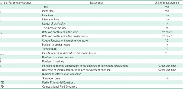
For a better understanding of the model, Table 1 summarizes the set of symbols, parameters and acro-nyms used in this proposal.
Consider a broiler house with a longitudinal wall (called here as “segment”) [0, L] ⊂ where L represents the facility length and a is the wall thickness. Two seg-ments, [–a, 0] and [L, L + a] represent the left-wall and right-wall, respectively. The diffusion coefficient in the walls is called σw and the diffusion coefficient in the broiler house is called σa. In addition, the control devic-es increase or decrease internal temperature u degrees per time unit, where u = u(x, t) is a function that de-pends on control decisions. This leads to the following diffusion problem:
∂
∂
(
)
=∂
∂
(
)
∈ −[
]
T t x t
T
x x t x a
w
, σ , ,
2
2 if 0 (1)
Table 1 − List of symbols, parameters and acronyms of the proposed controller.
Symbol/Parameter/Acronym Description Unit of measurement
t Time min
t0 Initial time min
tf Final time min
Δt Interval of time min
L Length of the facility m
a Thickness of the wall m
σw Diffusion coefficient in the walls m² min−1
σa Diffusion coefficient in the broiler house m² min −1
u Control function of internal temperature °C
x Position in broiler house m
T Temperature °C
Tideal Ideal temperature desired for the broiler house °C dj Number of control devices
N Number of devices
a Increase of internal temperature in the absence of connected exhaust fans °C per unit time
b Decrease of internal temperature per activation of each fan °C per unit time n Number of intervals for simulation
d Simulation time min
appropriately located sensors, interpolations and weath-er forecasting, establish the initial conditions for tem-perature at the facility and walls, as well as the bound-ary conditions that concern the external temperature from time t0 to tf ,
Step 2 – Trial controls: Choose “trial controls” di1 , ..., din, where dik∈ {d1, ... , dN} for all k = 1, ..., n.
Step 3 – Solve the PDE: Solve the problem (Equations 1 to 6) from t = t0 to t = tf, considering that the source function u(x, t) is determined by the choice of di1,..., din
in Step 2. Namely, in the solution process of Equations 1-6, assume that for all k = 1,..., n, if t ∈ [t0+ (k–1)d, t0
+ kd] the function u(x, t) is the one that corresponds to the control state dik.
Step 4 – Determine the score of the sequence of controls {di1 ,..., din}: Considering the values of the predicted temperatures T(x, t0 + kd) for x ∈ [0, L] and k = 1,..., n, computed in Step 3, compute a score a score for the sequence of controls decided in Step 2. If this score is not satisfactory yet, go to Step 2 to simulate the behav-ior of the system under new controls, or else, proceed to Step 5.
Step 5 – Implement the control, save for learning and stop, proceed implementing the control di1 and save T(x;
t0 + d), x ∈ [0, L]. After d units of real time, also save the real temperature inside the broiler house. Stop.
A flowchart of the conceptual algorithm is shown in Figure 1.
Note that the algorithm decides the best sequence of controls along the interval of real time [t0, tf], but it only imposes the implementation of the control comput-ed for the first interval [t0; t0 + d]. On one hand, consid-ering the whole interval [t0, tf ] to make decision instead of using merely [t0, t0 + d] prevents of making greedy decisions based only on the initial state at the facility, which could lead to overcooling or overheating. On the other hand, only the control decided for [t0; t0 + d] de-serves to be implemented in practice, as new data are coming permanently to the system that allows repeat-ing the simulations with better knowledge of the real environment.
After stopping the algorithm, the control di1 is implemented and “we wait” d units of real time before updating t0 and tf for running the algorithm again. This means that d is the number of time units in which the broiler house is subject to the control di1 before a new control optimization.
Optimization and learning
Optimization appears twice in the context of the algorithm implementation. The optimal choice of the controls di1, . . . din that maximizes the score comes from an optimization procedure whose characteristics depend on the type of control devices available in the broiler
∂
∂
(
)
=∂
∂
(
)
−(
)
∈[
]
T t x t
T
x x t u x t x L
a
, σ , , ,
2
2 if 0 (2)
∂
∂
(
)
=∂
∂
(
)
∈[
+]
T t x t
T
x x t x L L a
w
, σ , ,
2
2 if (3)
T (x, 0) given for all x∈ [–a, L + a] (4)
T (–a, t) = T(L + a, t) given for all t≥ 0 (5)
∂
∂
(
)
=∂
∂
(
)
2
2
2
2
0
T
x t
T
x L t
, , = 0 for all t≥ 0 (6) In other words, Equations (1) to (6) represent a dif-fusion problem (Welty et al., 2008) in the segment [–a,
L + a], where the diffusion coefficients are σw and σa in different regions. A boundary condition represents the external temperature and an initial condition that represents the initial temperature of the broiler house. Moreover, the temperature T(x, t) at the facility decreas-es if control u(x, t) is greater than zero, and increases otherwise.
The control function depends on the control de-vices. These control devices have a finite number of pos-sible states d0, d1, ... , dN. For example, dj may indicate that the number of connected exhaust fans is j, by as-suming that exhaust fans are the only control devices in the broiler house under analysis. A function udj (x, t) is associated to each possible control state dj:
udj (x, t) = a –jb (7) Therefore, in the absence of connected exhaust fans, internal temperature tends to increase a degrees per time unit, but the activation of each fan decreases the temperature b degrees per time unit.
The following conceptual algorithm describes how decisions are made. The algorithm runs on a continuous basis during the life of the broiler house (whole process of broiler rearing).
This algorithm is “conceptual” because, for the sake of simplicity, details concerning discretization and location of sensors are omitted. Inputs associated to the algorithm are: Tideal, temperature that depends on the age of chickens and type of the broiler house. The well-established value seeks to achieve thermal comfort of the animals to maximize their biological response and, therefore, weight gain. Moreover, it is assumed that L, a,
σw, σa and the functions uj are given for all j = 0, 1, ..., N. To fix date, time is measured in minutes and execu-tion of the algorithm starts when real “clock time” is t0. A simulation time is established of tf– t0 minutes (typically, one hour) and a number of intervals for simulation n
(typically, n = 10). Thus, d is defined as follows:
d = (tf– t0) / n (8)
Conceptual algorithm
house. For example, if all the devices are exhaust fans and their number is N , the controls dik can take the discrete values {0, 1, . . . , N}, corresponding to the number of exhaust fans connected at each d-interval. Therefore, the optimal controls are chosen from a set that contains (N + 1)nelements. For this case, it was ad-opted sequential coordinate search (Conn et al., 2009) as standard algorithm to obtain local optima. The score to be maximized takes into account the predicted tempera-tures at times t0 + d, . . . , t0 + nd. If Tideal is the ideal tem-perature desired for the broiler house, the score takes into account the approximation of inner temperatures to Tidealalong the instants t0 + kd. These approximations are weighted in a decreasing way with respect to k by maximizing the score given by:
− + − −
=
∑
k n
k ideal
n k T T
1
1
( ) (9)
where Tk is an average of the predicted temperatures in the sensors located in [0, L] at time t0 + kd.
The second instance where optimization appears is the Learning Process where the PDE model improves its ability to predict the real behavior of the system. In Step 5 of the algorithm, the predicted temperature at t0
+ d was saved and since the algorithm normally runs in much less than d time units, the real temperature at t0
+ d is saved later. Therefore, the real temperature can be compared against the predicted temperature every d time unit. Obviously, it is desired that these two vectors
of temperatures should be as close as possible. Thus, it is possible to modify the diffusion coefficients σw and σa and the dependence of u with respect to d in such a way that the difference between predicted and real tempera-tures is reduced. For this reduction, an additional opti-mization procedure is applied. As far as the algorithm runs in a real broiler house, these data allow successive improvements of the model, which, in turn, should im-prove efficiency of the control decisions. In other words, the model learns how to become more and more accu-rate during the execution of the algorithm.
Computational implementation
Solving the PDE
To solve the PDE (Equations 1 to 6), a straight-forward implicit difference scheme is implemented (Le Veque, 2007), which allows to use rather large values of time discretization preserving stability (Le Veque, 2007). The initial condition is obtained from measurements in several sensors (typically three) distributed in the broiler house followed by interpolation to get the initial temper-ature in [0, L]. The initial temperature within the walls is computed interpolating external and internal tempera-tures at the extremes of [0, L]. The boundary condition is given by the external temperature obtained from fore-casting at the weather station. The PDE must be solved for all trial controls di1, . . . , din. After the solution of each PDE for different controls is achieved, a score given by Equation (9) is attributed to trial di1, . . . , din. Successive trials, commanded by the coordinate-search scheme, lead to the computation of the effectively activated control di1. Finally, the left-wall is represented by the segment [-a, 0], where the right-wall is the segment [L,
L+a]. Therefore, a is the thickness of both walls. In this model, diffusion in both walls has identical coefficients, which are system parameters. In practice, the real value of a is not relevant and may be fixed arbitrarily, guided by numerical safeguards, since the effect of the walls is combined with the fitted diffusion parameters. Roughly speaking, under the accuracy degree of this model, a thick wall with a big diffusion coefficient has similar ef-fect as a thin wall with a small diffusion coefficient. In other words, different combinations of thickness and diffusion produce analogous temperature effects within the broiler house thus the precise determination of the diffusion within walls is not relevant.
Learning algorithm
Since the control di1, the optimization product of controls in Step 4 is effectively activated, after d units of time, current measurements of temperature in the broiler house are made, allowing to compare the mea-sured and predicted temperature by the PDE model. The measured temperature should be as close as pos-sible to the predicted one. Unfortunately, this is not the case, especially in the first stages of the effective system implementation in a broiler house. The
ing Algorithm modifies the model parameters σw, σaand the dependence of u with respect to di, for the predict-ed temperature at t0 + d coincides as much as possible with the real one obtained by the sensors. Moreover, it is not admissible abrupt modifications of the previous used parameters, which, especially after some hours of execution in the real environment, have already been the object of adjustments. For this reason, this Learning Algorithm consists of trying local random variations (10 % at most) around the already used parameters.
Calibration
Calibration is an optional procedure that can be executed at any time during the algorithm operation, as-suming that data on external and internal temperatures are registered during a comparative large period (24 h) together with the controls that were implemented along that period. In the calibration procedure, one tries to find the algorithmic parameters that produce the best fit of the temperatures computed by the Algorithm to the real temperatures collected so far.
Computer requirements
The installation of the system requires a laptop computer (3.5 GHz Intel Core i7 processor and 16GB 1600 MHz DDR3 RAM memory, running OS X Yosemite -version 10.10.4) to perform calculations. Sensors are re-quired to provide the temperature measurements in the broiler house. The model was programmed in Fortran 90. Codes were compiled by the GFortran, FORTRAN compiler of GCC (version 4.9.2) with O3 optimization directive enabled. Parameters a and b were initialized taking a = 0.02 and b = 0.01 and are updated through-out the learning process to fit better models to new data. The other main algorithmic parameters are σa, the diffu-sion coefficient in the broiler house and σw, the diffusion coefficient in the wall. In this case, they were initialized to σa= 1 and σw = 0.5, but they are continuously up-dated according to the learning process.
The pilot farm
Experiments were carried out in one pilot poul-try farm, in the municipality of Jundiaí, São Paulo State, Brazil (Latitude 23º11'11" S, Longitude 46º53'03" W). The broiler house is approximately 750 m above sea level and according to the international system of Köp-pen, the predominant climate in this region is Cwa (hot climate with a dry winter), with a mean air temperature of 22 °C in the hot season, and 15 °C in the cold season (registered by a local weather station managed by the Brazilian Institute of Meteorology).
The facility is the type Blue House (BH): the venti-lation system with negative pressure with an automatic controller FANCONTROL CC3, cooling pad system, and roof made of fiber cement, automatic feeding and drink-ing lines. Its dimensions are: length, 150.0 m; width, 15.0 m; sidewall height 2.5 m; and flock density average of 12 birds m−2.
Experiments
Controller simulations were performed on the pi-lot farm by comparing the evolution of the temperature measured by the model and the temperature registered by the automatic system when a rearing process was present. These experiments refer to different periods for different seasons of the year. Three experiments were designed and implemented.
Experiments were carried out by choosing differ-ent values of d and tf − t0. This means that the algorithm chooses the present control, which operates the follow-ing d minutes aiming to maximize the score in the fol-lowing 10d min.
Results and Discussion
Experiment 1
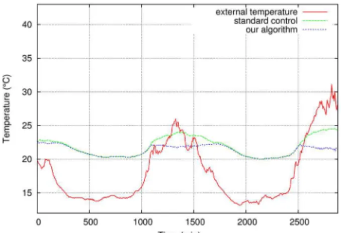
Two typical winter days: maximum external temperature was 32 °C around 14h00 and minimum 13 °C around 06h00. The initial average temperature at the facility was 22.2 °C. The ideal temperature ac-cording to the age of the birds (31-32 d old) is 22 °C (Cobb-Vantress, 2012). Results of simulation of the controller versus temperature registered by the sen-sors of the automatic controller are reported in Fig-ure 2.
During the night, when the external tempera-ture is lower than 22 °C, both algorithms keep similar internal temperatures. In this situation, exhaust fans are typically off, then, the algorithm is virtually in-active. However, during daytime, when temperatures rise, the proposed controller shows a better perfor-mance by keeping the internal temperature always below 22.4 °C, while the automatic controller reaches 24.5 °C. Considering these temperature peaks and comparing with the ideal temperature, the maximum discrepancy (bias) of the proposed model was 0.4 °C and for the automatic controller was 2.5 °C, respec-tively.
Figure 2 − Evolution of the temperatures for experiment 1 – Two
Experiment 2
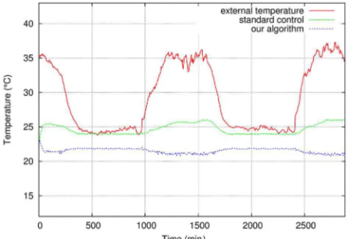
Two typical summer days: the maximal external temperature was 37.8 °C at 13h30 and the minimal was 24.0 °C between 00h00 and 06h00. The initial average temperature in the broiler house measured at 15h00 was 22.0 °C. Tideal was established at 22 °C as in experiment 1. Results are represented in Figure 3.
In this experiment, the difference between the two algorithms is clearer and more consistent. Even during the night, due to higher temperature than in the previous experiment, our algorithm shows a much bet-ter performance by keeping the inbet-ternal temperature of the broiler house around 22 °C. During the day, our al-gorithm always keeps the internal temperature below 22.4 °C, but the standard algorithm (automatic control-ler) allowed the internal temperature to reach 26.0 °C. Here, the maximum discrepancy of the proposed model was again 0.4 °C and 4 °C for the automatic controller.
The main reason for these different behaviors is that our model predicts the internal temperature in a reasonably accurate way and made decisions accord-ing to predictions, whereas the standard control takes decisions only according to current measurements. In addition, these measurements could be affected for sen-sor problems, such as a bad calibration, noise or signal transmissions inside the automatic controller.
Experiment 3
Long-term experiment - a simulation for 24 d dur-ing winter season (final stage of the reardur-ing process from 22 to 46 d old): the maximal external temperature was 35.6 °C and the minimal was 12.2 ° C. The initial aver-age temperature inside the facility was 22.5 °C at 15h00. Here, the average of the Tidealwas set at 21 ° C. Results are presented in Figure 4.
Once again, the results show the advantages of this proposal compared to the standard control mecha-nism. Consistently, our algorithm keeps the temperature closer to ideal during daytime, while the standard
con-trol mechanism, especially on hotter days, allows in-ternal temperature to reach 25.0 °C or even more. The discrepancy in comparison with the average of Tideal was approximately 1 °C for the model and 3.5 °C for the automatic controller, respectively.
If an average is calculated from the three experi-ments, the proposed model obtained a discrepancy in comparison with Tideal of approximately 0.6 °C and the automatic controller registered a mean value of 3.3 °C, respectively.
Finally, in this research, a real-time controller to keep and control adequate temperatures values in broiler houses was proposed. The system uses the PDE model to predict temperature inside the broiler house. The model is “semi-physical” on the sense that pre-serves some physical characteristics of the system, but it uses strong simplifications. Simplifications are used to allow computational implementation to be executed in real time. The optimization procedures involved in the model are fast enough to be compatible with the system operation and that the control system reacts in an adequate way to typical variations of temperature, keeping the internal temperature at acceptable levels. Its feasibility to support ventilation systems seems rea-sonable. Some empirical experiments have been de-signed to compare the model versus other automatic controllers on different farms. The proposed controller aims to provide maximum simplification of the physi-cal phenomenon compatible with good decisions. Oth-er controllOth-ers that could be based on linear or even nonlinear regression models may be excessively far from physical reality, whereas controllers based on full fluid mechanics are impractical for real-time pre-dictions, considering the cost of computer devices and response time. This proposal is fully portable and may be coupled to complex engineering of different sensor architectures. Moreover, the system is adaptable to dif-ferent dimensions of broiler houses due to its learning process for fitting parameters.
Figure 3 − Evolution of the temperatures for experiment 2 – Two
typical summer days.
Figure 4 − Evolution of the temperatures for experiment 3 – A
Therefore, future lines are focused on a complete evaluation of the system. These lines refer to more test-ing activities in the field. Although the sensitivity and stability analysis of the proposed controller is beyond the scope of this work, a theoretical analysis will be ad-dressed in a mathematical-oriented future work, due to the importance of the topic. From the practical view-point, in the range of parameters that corresponds to broiler houses, stability and sensitivity seemed to be quite satisfactory.
The methodological approach used in this work can be applied in many real problems, involving com-plex physical phenomena, mainly in problems related to environmental control for livestock production that requires judicious simplifications for reliable modeling. Many human decisions require real-time optimization procedures and self-correcting strategies increase accu-racy and help as supporting tools in the decision-making process.
Acknowledgments
This work was supported by the program Pronex of the Brazilian National Council for Scientific and Techno-logical Development (CNPq) and Rio de Janeiro Research Foundation (FAPERJ) E-26/111.449/2010-APQ1, São Pau-lo Research Foundation (FAPESP) (grants 2010/10133-0, Cepid-Cemeai 2011-51305-02, 2013/03447-6, 2013/05475-7, 2013/07375-0 and 2013/21112-1) and Bra-zilian National Council for Scientific and Technological Development (CNPq) grant 144669/2013-7.
References
Anderson, J.D. 1995. Computational Fluid Dynamics: The Basics with Applications. McGraw-Hill, New York, NY, USA. Bustamante, E.; García-Diego, F.J.; Calvet, S.; Estellés, F.; Beltrán,
P.; Hospitaler, A.; Torres, A.G. 2013. Exploring ventilation efficiency in poultry buildings: the validation of computational fluid dynamics (CFD) in a cross-mechanically ventilated broiler farm. Energies 6: 2605-2623.
Cobb-Vantress. 2012. Broiler management guide. Available at:http://www.cobb-vantress.com/docs/default-source/ management-guides/broiler-management-guide.pdf [Accessed: May 31, 2017]
Conn, A.R.; Scheinberg, K.; Vicente, L.N. 2009. Introduction to Derivative-Free Optimization. SIAM, Philadelphia, PA, USA. (MPS-SIAM Series on Optimization).
Donkoh, A. 1989. Ambient temperature: a factor affecting performance and physiological response of broiler chickens. International Journal of Biometeorology 33: 259-265.
Fletcher, C.A.J.; Fletcher, C. 1988. Computational Techniques for Fluid Dynamics. Springer-Verlag, Heidelberg, Germany. Le Veque, R.J. 2007. Finite Difference methods for Ordinary
and Partial Differential Equations: Steady State and Time Dependent Problems. SIAM, Philadelphia, PA, USA.
Razuki, W.M.; Mukhlis, S.A.; Jasim, F.H.; Hamad, R.F. 2011. Productive performance of four commercial broilers genotypes reared under high ambient temperatures. International Journal of Poultry Science 10: 87-92.
Reboiro-Jato, M.; Glez-Dopazo, J.; Glez, D.; Laza, R.; Galvez, J. F.; Pavon, R.; Glez-Peña, D.; Fernandez-Rivarola, F. 2011. Using inductive learning to assess compound feed production in cooperative poultry farms. Expert Systems with Applications 38: 14169–14177.
Renaudeau, D.; Collin, A.; Yahav, S.; Basilio, V.; Gourdine, J.L.; Collier, R.J. 2012. Adaptation to hot climate and strategies to alleviate heat stress in livestock production. Animal 6: 707– 728.
Rojano, F.; Bournet, P.E.; Hassouna, M.; Robin, P.; Kacira, M.; Choi, C.Y. 2015. Modelling heat and mass transfer of a broiler house using computational fluid dynamics. Biosystems Engineering 136: 25–38.
Welty, J.; Wicks, C.E.; Rorrer, G.L.; Wilson, R.E. 2008. Fundamentals of Momentum, Heat and Mass Transfer. John Wiley, New York, NY, USA.