Estimation of the properties of a range-dependent ocean environment. A simulation study

CINTAL - Centro de Investiga¸

c˜

ao Tecnol´

ogica do Algarve

Universidade do Algarve

Estimation of the Properties of a

Range-Dependent Ocean Environment:

a Simulation Study

V. Corr´

e

Rep 03/01 - SiPLAB 26/October/2001

University of Algarve tel: +351-289800131

Campus da Penha fax: +351-289864258

8000, Faro, cintal@ualg.pt

Work requested by CINTAL

Universidade do Algarve, Campus da Penha, 8000 Faro, Portugal

tel: +351-289800131, cintal@ualg.pt, www.ualg.pt/cintal Laboratory performing SiPLAB - Signal Processing Laboratory

the work Universidade do Algarve, FCT, Campus de Gambelas,

8000 Faro, Portugal

tel: +351-289800949, info@siplab.uceh.ualg.pt, www.ualg.pt/uceh/adeec/siplab

Projects ATOMS - FCT, PDCTM/P/MAR/15296/1999

Title Estimation of the properties of a range-dependent ocean

en-vironment: a simulation study

Authors V. Corr´e

Date October 26, 2001

Reference 03/01 - SiPLAB

Number of pages 22 (twenty two)

Abstract This report describes a simulation study to estimate the range and depth variations of ocean acoustic properties. The es-timation is based on matched-field inversion. Results show the feasibility of detecting the presence of an abnormal-temperature water entity.

Clearance level UNCLASSIFIED

Distribution list SiPLAB (1), CINTAL (2), FCT (1)

Total number of copies 4 (four) Copyright Cintal@2001

III

Contents

List of Figures V

1 Introduction 6

2 Model of the range-dependent environment 7

3 Inversion method 9

3.1 Forward model . . . 9 3.2 Cost function . . . 9 3.3 Hybrid inversion method . . . 9

4 Simulated data 11

4.1 Sensitivity study . . . 11 4.2 Inversion results . . . 14 4.2.1 Observations and discussion . . . 14

5 Conclusions and further work 21

List of Figures

2.1 Waveguide model . . . 8

4.1 Sound speed profiles used to generate simulated data . . . 12

4.2 Variations of the misfit with individual parameters . . . 13

4.3 Result of 10 inversions for scenario 1 . . . 15

4.4 Result of 10 inversions for scenario 2 . . . 16

4.5 Result of 10 inversions for scenario 3 . . . 17

4.6 Result of 10 inversions for scenario 4 . . . 18

Chapter 1

Introduction

The properties of coastal ocean environments often show a high variability with time and space (range, cross-range, depth). While direct measurements of these properties can be time consuming and offer usually a poor coverage, acoustic inversion represents an attractive alternative to estimate these properties [1, 2].

The ATOMS project aims to study a coastal environment featuring a cold water filament among warmer waters. One of the major goals of the project is to show that it is possible to detect and characterize such a filament in space and time using an acoustic inversion method.

The current work is a preliminary study in the project as it deals with a simplified approach to the global problem:

1- The particular case of a 2-D environment (vertical slice) is investigated. This means that we consider only the variations of the properties in the vertical plane defined by the acoustic source and a vertical line array.

2- Time variability is not considered.

3- Although they are based on experimental records of a filament [3], the data used here are only simulated data.

This report is organized as follows. The waveguide model adopted to represent the range-dependent environment is defined in Chapter 2. Chapter 3 describes the inversion method. The method is based on matched-field processing [4], a powerful technique that makes use of the spatial properties of the acoustic full field to solve the problem of parameter estimation. Chapter 4 presents the simulated data set, as well as inversion results. Finally, some conclusions are given in Chapter 5.

Chapter 2

Model of the range-dependent

environment

In nature, coastal ocean environments are complex waveguides. As their properties can vary continuously with space and time, a discretized model of such environments is al-ways an approximation. The choice of a model depends, among others, on the expected variations of the properties and on the desired accuracy of their estimates. The choice of a model is therefore case dependent.

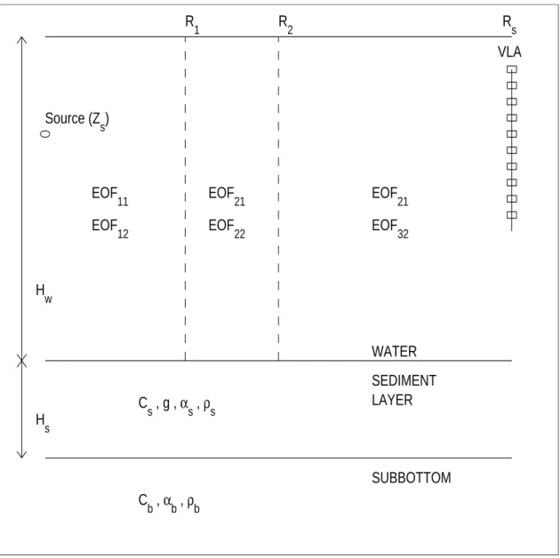
For the particular case of this study, we are interested primarily in detecting the pres-ence of a water temperature anomaly, and then possibly studying its variations with space and time. We thus chose a simple representation of the range-dependent environment.

In our model, the water waveguide is divided into three vertical sectors, the middle sec-tor modeling the water with abnormal temperature. In each of the secsec-tor, the temperature and salinity (and therefore the water sound speed and density) are range independent. Variations of the sound speeds with depth are given through EOFs [5]. Although the model can take into account a variable bathymetry, in this study we consider only the case of an environment with constant water depth (Hw). The ocean bottom is modeled as a sediment layer laying over the subbottom. The parameters to characterize the bottom are the layer thickness (Hs), the P-wave velocity (Cs) at the seafloor, the linear velocity gradient (g) in the layer, the attenuation of the P-wave (αs) and the density (ρs) in the layer, as well as the P-wave velocity (Cb), attenuation (αb) and density (ρb) in the sub-bottom. These parameters are assumed range independent. Shear-wave parameters are not considered.

8 CHAPTER 2. MODEL OF THE RANGE-DEPENDENT ENVIRONMENT VLA EOF 11 EOF 12 EOF 21 EOF 22 EOF 21 EOF 32 R 1 R2 Rs Source (Z s) H w H s C s , g , αs , ρs C b , αb , ρb WATER SEDIMENT LAYER SUBBOTTOM

Chapter 3

Inversion method

In order to recover some, or all, of the waveguide parameters, an inversion method based on matched-field processing was chosen. The idea behind matched-field inversion is simple and the problem is casted as an optimization problem. Instead of inverting the pressure fields, one looks for the model of parameters that minimizes the difference between the measured field and the replica field calculated for this particular model.

3.1

Forward model

In this study, all pressure fields (replica as well as simulated data) were calculated with the normal mode code PROSIM [6].

3.2

Cost function

To quantify the misfit between data and replica fields, the frequency-incoherent Bartlett processor was used. This processor is defined as follows. Let ˆD(f ) represent the normalized data pressure field measured at frequency f , and ˆP∗(m, f ) represent the normalized replica field calculated for the model of parameters m. When the fields have Nf frequency components, the cost function to minimize is given by:

E(m) = 1₋ 1 Nf Nf X k=1 | ˆP∗(m, fk) ˆD(fk)|2. (3.1)

3.3

Hybrid inversion method

The inversion consists in sampling the parameter space to determine the model of param-eters that minimizes E(m). This can be a challenging issue: the parameter space is large, some correlations may exist between parameters and the problem is non linear.

10 CHAPTER 3. INVERSION METHOD

Usually, an exhaustive search is not a suitable approach to solve the problem. In-stead, hybrid methods can efficiently sample complex parameter spaces [7, 8]. The hybrid method used here is the simplex genetic algorithm (SGA) method which combines a global search, the genetic algorithm (GA) [9], and a local search, the downhill simplex (DHS) method [10]. From a population of models, a subsample (simplex) is selected. GA oper-ations and then DHS are applied to the simplex of models. The model with the lowest misfit replaces the model in the population with the largest misfit. The process is repeated until i) the population has converged or ii) a predetermined number of forward modelings has been reached. A final DHS is run with a simplex of models. One of these models corresponds to the best model encountered during the inversion. The other models are randomly chosen in the entire parameter space.

Chapter 4

Simulated data

The inversion method was tested on a simulated data set obtained for realistic conditions. The simulated environment was based on the waveguide model shown in Fig. 2.1. The source was located 200 km from a vertical line array made of 10 receivers equally space and spanning the 20-290 m of the water column. The source depth was set to 109 m. Five frequencies spanning the 100-500 Hz band were used. Temperatures and salinities measured in an area exhibiting a cold filament [3] were used to calculate sound speed profiles in three distinct sectors: a cold water sector, and two warmer sectors around. As multiple sample points are usually necessary to accurately represent the sound speed profiles, a direct estimation of these points can lead to a parameter space too large to be reasonably sampled. Instead, using EOFs to describe the profiles is more efficient. When multiple measurements of a profile are available, they can be used to generate a set of eigenfunctions Fi which allow a simple representation of the sound speed v at depth z:

v(z) = v(z) + I

X

i=1

βiFi(z). (4.1)

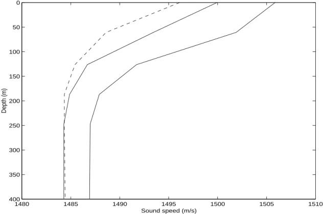
In this equation, v(z) is the average speed and βi are the coefficients associated with the eigenfunctions. These coefficients represent the unknown parameters to estimate. Usually, a few eigenfunctions (I=2 or 3) are sufficient to represent accurately the sound speed. Here, to simulate multiple measurements of the sound speed profiles, several realizations of zero-mean, Gaussian-distributed random noise were added to the three original profiles. The standard deviation of the noise was 0.5 m/s. The three “true” sound speed profiles are shown in Fig. 4.1. They were obtained using two EOFs per sector.

Values of all geoacoustic parameters of the true environment are given in Tab. 4.1.

4.1

Sensitivity study

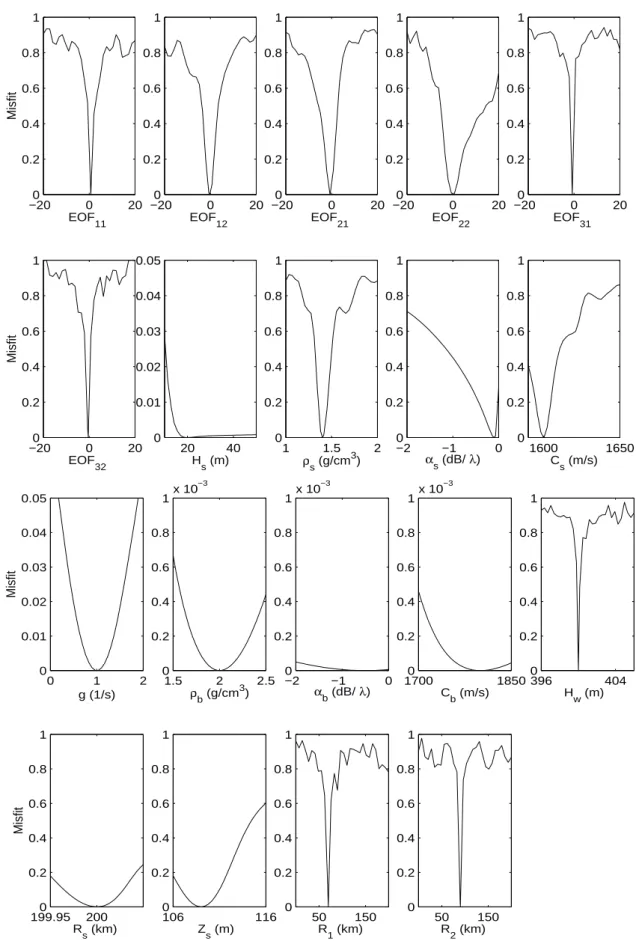
The pressure field is not equally sensitive to all parameters. For simulated data, one way to quantify the different sensitivities is to study the variations of the cost function close to the global minimum. By letting only one parameter vary at a time while the others are fixed to their true values,it is possible to see how the parameter affects the cost function. The variations of the misfit with the waveguide and source parameters are given

12 CHAPTER 4. SIMULATED DATA 1480 1485 1490 1495 1500 1505 1510 0 50 100 150 200 250 300 350 400 Sound speed (m/s) Depth (m)

Figure 4.1: Sound speed profiles used to generate simulated data. The dashed line repre-sents the profile of the middle sector.

Table 4.1: True environment.

Parameter True value

EOF11 0.6884 EOF12 -0.2849 EOF21 -0.6443 EOF22 0.0746 EOF31 -0.7965 EOF32 -0.4228 Hw 400 m Hs 20 m R1 70 km R2 90 km Cs 1600 m/s g 1 1/s ρs 1.4 g/cm3 αs 0.1 dB/λ Cb 1800 m/s ρb 2. g/cm3 αb 0.5 dB/λ

in Fig. 4.2. The effect of the subbottom parameters is order of magnitude smaller than the EOFs for example. Based of these results, we studied different scenarios of inversion with increasing number of unknown parameters, starting with the most sensitive ones.

4.1. SENSITIVITY STUDY 13 −200 0 20 0.2 0.4 0.6 0.8 1 Misfit EOF₁₁ −200 0 20 0.2 0.4 0.6 0.8 1 EOF₁₂ −200 0 20 0.2 0.4 0.6 0.8 1 EOF₂₁ −200 0 20 0.2 0.4 0.6 0.8 1 EOF₂₂ −200 0 20 0.2 0.4 0.6 0.8 1 EOF₃₁ −200 0 20 0.2 0.4 0.6 0.8 1 Misfit EOF 32 20 40 0 0.01 0.02 0.03 0.04 0.05 H s (m) 1 1.5 2 0 0.2 0.4 0.6 0.8 1 ρ_s (g/cm3) −2 −1 0 0 0.2 0.4 0.6 0.8 1 α_s (dB/ λ) 1600 1650 0 0.2 0.4 0.6 0.8 1 C s (m/s) 0 1 2 0 0.01 0.02 0.03 0.04 0.05 Misfit g (1/s) 1.5 2 2.5 0 0.2 0.4 0.6 0.8 1x 10 −3 ρ_b (g/cm3) −2 −1 0 0 0.2 0.4 0.6 0.8 1x 10 −3 α_b (dB/ λ) 1700 1850 0 0.2 0.4 0.6 0.8 1x 10 −3 C b (m/s) 396 404 0 0.2 0.4 0.6 0.8 1 H w (m) 199.950 200 0.2 0.4 0.6 0.8 1 Misfit R_s (km) 106 116 0 0.2 0.4 0.6 0.8 1 Z_s (m) 50 150 0 0.2 0.4 0.6 0.8 1 R₁ (km) 50 150 0 0.2 0.4 0.6 0.8 1 R₂ (km)

Figure 4.2: Variations of the misfit with individual parameters, the remaining parameters being fixed to their true values. Note the different misfit scales.

14 CHAPTER 4. SIMULATED DATA

4.2

Inversion results

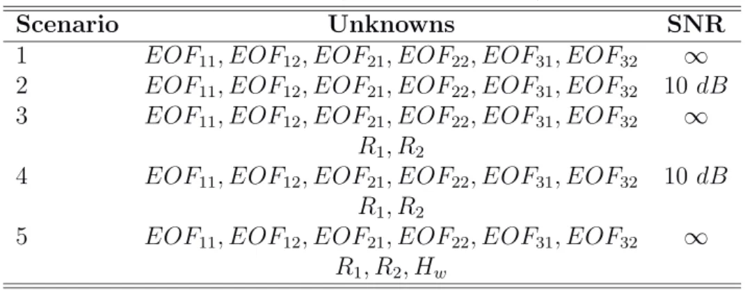
The different scenarios investigated are described in Tab. 4.2. The known parameters were set to their true values. Therefore, in absence of noise in the data, the global minimum was zero (or the machine accuracy). In scenario 2 and 4, zero-mean, Gaussian-distributed random noise (N (f )) was added to the data. The signal-to-noise ratio was given by:

SN R = 10_{× log}10   PNf i=1|P (fi)|2 PNf i=1|N(fi)|2  . (4.2)

The parameter search intervals were the same than the intervals used in the sensitivity study. Although the search interval for the EOF coefficients was large, large variations (> 5m/s) of the sound speed around the mean speed were penalized.

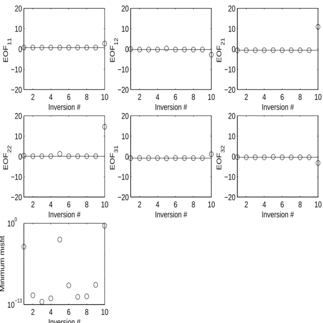
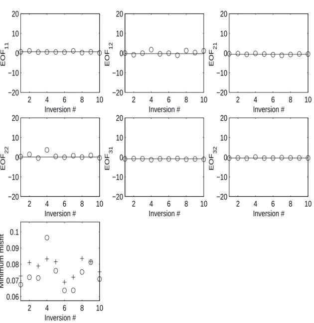
For each scenario, series of inversions (10) were repeated in order to check the consistency of the inversion algorithm results. For each inversion with scenario 2 or 4, a different ran-dom noise realization was used while keeping a constant SNR. Final parameters estimates and the corresponding misfit are given in Fig. 4.3 to 4.7.

Each inversion of the first two scenarios involved between 3000 to 3500 forward calcu-lations. As the number of unknowns increased, the number of these calculations was increased as well (_{∼4500 for scenario 5).}

Table 4.2: List of scenarios investigated

Scenario Unknowns SNR

1 EOF11, EOF12, EOF21, EOF22, EOF31, EOF32 ∞ 2 EOF11, EOF12, EOF21, EOF22, EOF31, EOF32 10 dB 3 EOF11, EOF12, EOF21, EOF22, EOF31, EOF32 ∞

R1, R2

4 EOF11, EOF12, EOF21, EOF22, EOF31, EOF32 10 dB R1, R2

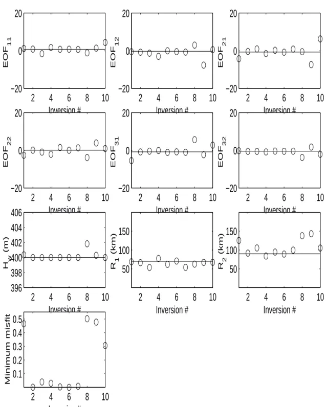
5 EOF11, EOF12, EOF21, EOF22, EOF31, EOF32 ∞ R1, R2, Hw

4.2.1

Observations and discussion

Scenario 1: Except for the 10th inversion, the final estimates are close to the true values and the corresponding misfit is close to zero.

Scenario 2: In general, in presence of noise, the global misfit is not obtained with the true parameter values. As shown in Fig. 4.4, the minimum misfits found are smaller than the misfit calculated with the true values. However, the parameter estimares are still close to the true values.

Scenario 3: In two of the inversions, the algorithm failed in finding a very low misfit. The relative errors ((mest− mtrue)/mtrue) are less than 30% for R1 and 15% for R2.

Scenario 4: Like in scenario 2, the algorithm was efficient enough to determine misfits smaller than the misfit with the true parameter values. However, the results show some significant variability, indicating that the SGA algorithm was not tuned in an optimum

4.2. INVERSION RESULTS 15 2 4 6 8 10 −20 −10 0 10 20 Inversion # EOF 11 2 4 6 8 10 −20 −10 0 10 20 Inversion # EOF 12 2 4 6 8 10 −20 −10 0 10 20 Inversion # EOF 21 2 4 6 8 10 −20 −10 0 10 20 Inversion # EOF 22 2 4 6 8 10 −20 −10 0 10 20 Inversion # EOF 31 2 4 6 8 10 −20 −10 0 10 20 Inversion # EOF 32 2 4 6 8 10 10−13 100 Minimum misfit Inversion #

Figure 4.3: Result of 10 inversions for scenario 1. The circles represent the final param-eter estimates and the corresponding misfit. The solid lines represent the true paramparam-eter values.

16 CHAPTER 4. SIMULATED DATA 2 4 6 8 10 −20 −10 0 10 20 Inversion # EOF 11 2 4 6 8 10 −20 −10 0 10 20 Inversion # EOF 12 2 4 6 8 10 −20 −10 0 10 20 Inversion # EOF 21 2 4 6 8 10 −20 −10 0 10 20 Inversion # EOF 22 2 4 6 8 10 −20 −10 0 10 20 Inversion # EOF 31 2 4 6 8 10 −20 −10 0 10 20 Inversion # EOF 32 2 4 6 8 10 0.06 0.07 0.08 0.09 0.1 Minimum misfit Inversion #

Figure 4.4: Result of 10 inversions for scenario 2 (SN R = 10dB). In the last panel, the crosses represent the misfits with the true values.

4.2. INVERSION RESULTS 17 2 4 6 8 10 −20 −10 0 10 20 Inversion # EOF 11 2 4 6 8 10 −20 −10 0 10 20 Inversion # EOF 12 2 4 6 8 10 −20 −10 0 10 20 Inversion # EOF 21 2 4 6 8 10 −20 −10 0 10 20 Inversion # EOF 22 2 4 6 8 10 −20 −10 0 10 20 Inversion # EOF 31 2 4 6 8 10 −20 −10 0 10 20 Inversion # EOF 32 2 4 6 8 10 50 100 150 Inversion # R 1 (km) 2 4 6 8 10 50 100 150 Inversion # R 2 (km) 2 4 6 8 10 0.02 0.04 0.06 0.08 0.1 0.12 0.14 Minimum misfit Inversion # Figure 4.5: Result of 10 inversions for scenario 3.

18 CHAPTER 4. SIMULATED DATA 2 4 6 8 10 −20 −10 0 10 20 Inversion # EOF 11 2 4 6 8 10 −20 −10 0 10 20 Inversion # EOF 12 2 4 6 8 10 −20 −10 0 10 20 Inversion # EOF 21 2 4 6 8 10 −20 −10 0 10 20 Inversion # EOF 22 2 4 6 8 10 −20 −10 0 10 20 Inversion # EOF 31 2 4 6 8 10 −20 −10 0 10 20 Inversion # EOF 32 2 4 6 8 10 50 100 150 Inversion # R 1 (km) 2 4 6 8 10 50 100 150 Inversion # R 2 (km) 2 4 6 8 10 0.1 0.2 0.3 0.4 0.5 Minimum misfit Inversion # Figure 4.6: Result of 10 inversions for scenario 4 (SN R = 10dB).

4.2. INVERSION RESULTS 19

2

4

6

8

10

−20

0

20

Inversion #

2

4

6

8

10

−20

0

20

Inversion #

2

4

6

8

10

−20

0

20

Inversion #

2

4

6

8

10

−20

0

20

Inversion #

2

4

6

8

10

−20

0

20

Inversion #

2

4

6

8

10

−20

0

20

Inversion #

2

4

6

8

10

396

398

400

402

404

406

Inversion #

2

4

6

8

10

50

100

150

Inversion #

2

4

6

8

10

50

100

150

Inversion #

2

4

6

8

10

0.1

0.2

0.3

0.4

0.5

Inversion #

20 CHAPTER 4. SIMULATED DATA

manner.

Scenario 5: As in scenario 4, the SGA algorithm does not seem to be tuned properly, as low misfits are not found systematically. The estimates of the water depth is nevertheless very good.

In the simplest case where only the EOF coefficients were not known, the SGA inversion provided good estimates of the parameters. Although this case is not realistic, it shows us that the data contain the information necessary to recover some elements of a range-dependent environment. For the range of frequencies used here, the range-range-dependent environment is not equivalent to an “average” range-independent environment.

As we are interesting in studying the variations of the middle sector, the scenarios in-cluding the sector limits are more interesting. In the different cases studied here, it was possible to find relatively good estimates of these limits. However, the accuracy found may not be sufficient to study their variations later on, and improvement will be neces-sary. The hability to recover the properties of the middle sector depends on the degree of insonification of the sector. The smaller the sector, the fewer the acoustic energy samples the region. Therefore, the less information available to estimate the properties. However, in reality, there is no control over the size of the middle sector. Therefore little can be done in this domain for improvement. On the other hand, it is possible to chose the locations of the source and receivers which have also a significant effect on the spatial distribution of the sound in the waveguide.

Chapter 5

Conclusions and further work

In this study, we investigated a simple case of acoustic inversion in a range-dependent environment. Simulated data were generated for an environment composed of three range-independent sectors. Parameters to estimate were two EOF coefficients of the sound speed profiles per sector, as well as the range limits of the middle sector. Using a matched-field inversion method, it was possible to recover the EOF coefficients fairly well. Very accurate estimates of the range limit parameters appeared more difficult to obtain. However, considering the large interval search used in this study for these parameters, the estimates obtained represent a good first approximation. Such estimates could be used in a second inversion process to refine the results for example.

As one looked for both the sound speed profiles and the middle sector limits, the degree of freedom in the problem was high. The recovery of the range-dependent pattern is therefore a very encouraging result.

Future work includes 1) increasing the number of unknowns (source location), 2) op-timizing the location of source and receivers, 3) studying the effect of model mismatch (true waveguide more complex than the modeled one) and 4) investigating the use of 2-D EOF coefficients to model the depth and range variations of the water sound speed.

Bibliography

[1] C.S. Chiu, J.H. Miller, W.W.Denner and J.F.Lynch, “Forward modeling of the Bar-ents Sea tomography vertical line array data and inversion highlights”, Full field inversion methods in ocean and seismo-acoustics, Kluwer Academic Publishers, pp 237-242, 1995.

[2] A. Tolstoy and O. Diachok, “Acoustic tomography via matched field processing”, J.Acoust.Soc.Am., 89, pp 1119-1127, 1991.

[3] R.K. Dewey, J.N. Moun, C.A. Paulson, D.R. Caldwell and S.D. Pierce, “Structure and dynamics of a coastal filament”, J.Geophys.Res., 96(C8), pp 14885-14907, 1991. [4] A.B. Baggeroer, W.A. Kuperman and P.N. Mikhalevsky, “An overview of matched

field methods in ocean acoustics”, IEEE J.Ocean.Eng., 18, pp. 401–424, 1993. [5] R.E. Davis, “Predictability of sea surface temperature and sea level pressure

anoma-lies over the north pacific ocean”, J.Phys.Ocean., 6, pp. 249-266, 1976.

[6] F. Bini-Verona, P.L. Nielsen and F.B. Jensen, “PROSIM broadband normal-mode model”, SACLANTCEN Memorandum serial number No.:SM-358.

[7] M.R. Fallat and S.E. Dosso, “Geoacoustic inversion via local, global and hybrid algorithms”, J.Acoust.Soc.Am., 105, pp 3219-3230, 1999.

[8] P. Gerstoft , “Inversion of acoustic data using a combination of genetic algorithms and the Gauss-Newton approach”, J.Acoust.Soc.Am., 97, pp 2181-2190, 1995. [9] D.E. Goldberg, Genetic algorithms in search, optimization and machine learning

Addison Welssey Publishing company, Reading, MA, 1989.

[10] W.H. Press, B.P. Flannery, S.A. Teukolsky and W.T. Vetterling, Numerical Recipes - The Art of Scientific Computing 2nd ed., Cambridge University Press, Cambridge, 1992.