By
YOUNES NIKDELAN
SUBMITTED IN PARTIAL FULFILLMENT OF THE REQUIREMENTS FOR THE DEGREE OF
DOCTOR OF MATHEMATICS AT
INSTITUTO NACIONAL DE MATEM ´ATICA PURA E APLICADA (IMPA) RIO DE JANEIRO, BRAZIL
SEPTEMBER 2014
c
INSTITUTO NACIONAL DE MATEM ´ATICA PURA E APLICADA (IMPA)
The undersigned hereby certify that they have read and recommend to IMPA for acceptance a thesis entitled “ Darboux-Halphen-Ramanujan Vector Field on a Moduli of Calabi-Yau Manifolds” by YOUNES NIKDELAN in partial fulfillment of the requirements for the degree of Doctor of Mathematics.
Dated: September 2014
Research Supervisor:
Hossein Movasati (IMPA)
External Examiners:
Bruno Scardua (UFRJ)
Mauricio Correa (UFMG)
Examing Committee:
Alcides Lins Neto (IMPA)
Mikhail Belolipetsky (IMPA)
Date: September 2014
Author: YOUNES NIKDELAN
Title: Darboux-Halphen-Ramanujan Vector Field on a
Moduli of Calabi-Yau Manifolds
Degree: Ph.D. Convocation: September Year: 2014
Signature of Author
To the Memory of My Beloved Brother ”SADEGH”...
Table of Contents v
Abstract vii
Acknowledgements ix
Introduction 1
1 Historical Backgrounds 7
1.1 Problem Statement . . . 7
1.2 Darboux . . . 12
1.3 Halphen . . . 14
1.4 Ramanujan . . . 15
2 Hodge Theory and Families 17 2.1 Local Systems and Integrable Connections . . . 17
2.2 Hodge Structure . . . 19
2.3 de Rham Cohomology and Hodge Filtration . . . 20
2.4 Families and Complex Deformations . . . 25
2.5 Gauss-Manin Connection and Griffiths Transversality . . . 26
2.6 Intersection Forms . . . 28
3 Picard-Fuchs Equation as a Self-Dual Linear Differential Equation 31 3.1 Differential Operators . . . 31
3.2 Picard-Fuchs Equation . . . 36
3.3 Self-Duality . . . 37
4 Calabi-Yau Manifolds 43 4.1 Definitions and Properties . . . 46
4.2 Families and More Examples . . . 51
5 Darboux-Halphen-Ramanujan Vector Field 53
5.1 Odd Case . . . 54
5.2 Even Case . . . 64
5.3 Five-Dimensional Case . . . 66
5.4 Three-Dimensional Case . . . 71
6 Related Problems 75 6.1 The Moduli Space . . . 75
6.2 Yukawa Coupling . . . 75
6.3 Geometric Structure of Calabi-Yau 5-Folds . . . 76
6.4 Semi-complete Vector Fields . . . 77
A Tables 81
Bibliography 84
This research was intended as an attempt to obtain an ordinary differential equation H from a linear differential equation L. We work on a Calabi-Yau n-fold W whose complex deformation is one dimensional and middle complex de Rham cohomology HdRn (W;C) is (n+ 1)-dimensional. Moreover, we suppose that the Picard-Fuchs equation L associated with the unique nowhere vanishing holomorphicn-formω onW is of order n+ 1. As a first result, we prove that Lis self-dual.
Next, we define T to be the moduli of W together with a basis of Hn
dR(W;C), where
the basis is required to be compatible with the Hodge filtration ofHdRn (W;C); furthermore, the intersection form matrix in this basis is constant. Then in our second result, we verify the existence of a unique vector field H on T that satisfies certain properties. Indeed,
the ordinary differential equation given by H is a generalization of differential equations introduced by Darboux, Halphen and Ramanujan.
Keywords: Darboux-Halphen-Ramanujan vector field, Hodge structure, Picard-Fuchs equation, Gauss-Manin connection.
First I would like to express my very great appreciation to Prof. Hossein Movasati, my supervisor, who introduced to me this area and always was available and I used his valu-able and constructive suggestions and helps during the planning and development of this research.
I wish to thank Khosro M. Shokri, for constructive conversations that we had during my research. I also was benefited by the supports of Professors Alcides Lins Neto and Marcos Dajczer that I express my gratitude to them.
I had the pleasure to do some courses with Professors Alcides Lins Neto, Marcelo Viana, Marcos Dajczer, Jorge Vitrio Pereira, Henrique Bursztyn and Luis Adrian Florit, and I thank them for teaching and motivating me more.
The author is greatly indebted to his master supervisor Prof. S. M. B. Kashani, for his continuous supports.
I would like to thank IMPA and its staffs for preparing such an excellent academic environment, and also I am grateful to have economic supports of ”CNPq-TWAS Fellowships Programme”.
A special thanks to my family. My sincerest thanks goes to my mum and my dad for their patience, love and unconditional supports and also to my brothers Akbar, Asghar, Ahmad, Amin and to my sisters Ashraf, Fatemeh, Tayebeh. Words can not express how grateful I am to my beloved wife Jhoana, who was always there cheering me up and stood by me through the happiness and sadness.
Finally, I wish to thank all my friends who I spent gratifying and delightful time with them. In particular: Ali Golmakani, Kyara, Felipe Macias, Kari Marin, Sajad, Vahideh, Hamed, Ana, Vivi, Marco, Francisco, Vandi, Ruben, Leandro, Anita, Alex, Roberto, Mehdi, Mahdi, Sina and Ali.
Rio de Janeiro, Brasil Younes Nikdelan
July 27, 2014
Introduction
Calabi-Yau manifolds are defined as compact connected K¨ahler manifolds whose canonical bundle is trivial, though many other equivalent definitions are sometimes used (see Theorem 4.3). They were named ”Calabi-Yau manifold” by Candelas et al. (1985) [9] after E. Calabi (1954) [6, 7], who first studied them, and S. T. Yau (1976) [42], who proved the Calabi conjecture that says Calabi-Yau manifolds accept Ricci flat metrics. In this text, we sup-pose that for an n-dimensional Calabi-Yau manifoldhp,0 = 0, 0< p < n, where hp,q refers to (p, q)-th Hodge number of Calabi-Yau manifold. It is clear that the connectedness of a Calabi-Yau manifold and the triviality of its canonical bundle imply thath0,0=hn,0 = 1.
Since introducing Calabi-Yau manifolds, a lot of work has been done on these manifolds by mathematicians an physicists. The importance of Calabi-Yau manifolds were found more, after discovering the concept of mirror symmetry by physicists. Mirror symmetry is a conjecture that says there exist mirror pairs of Calabi-Yau manifolds. Quite roughly, we should think of W and ˜W as being a mirror pair if there is an isomorphism between MKah(W) and Mcmplx( ˜W), where MKah(X) and Mcmplx(X), resp., refer to K¨ahler and complex moduli, resp., of a K¨ahler manifold X. One of important and primary of these works in 1991 was given by Candelas et al. in [8], where they used the mirror symmetry to predict the number of rational curves on quintic 3-folds. In some other works, such as [1, 2, 11, 15, 27, 28, 29], authors construct new Calabi-Yau manifolds and their mirrors, and then they investigate other properties of these constructed manifolds.
The main work of this thesis, which is motivated by linear differential equations in-troduced by Darboux, Halphen and Ramanujan, is to present a vector field H with some special properties on a moduli space of Calabi-Yau manifolds and we call it DHR vector field. To know more about DHR vector field we start with 1-dimensional Calabi-Yau mani-folds, which are elliptic curves. LetE be an elliptic curve overC. Then the Hodge filtration (for definition see §2.3) F• of the first de Rham cohomology group (for definition see§2.5) HdR1 (E) is given as follow,
{0}=F2 ⊂F1 ⊂F0=HdR1 (E), dimC(Fi) = 2−i.
Let T be the moduli of the pair (E,[α1, α2]), in which α1 ∈ F1, α2 ∈ F0 \F1, and the
matrix of their intersection forms (for definition see §2.6) is as follow,
(hαi, αji)1≤i,j≤2=
0 1
−1 0
.
To be more precise, if we consider the Weierstrass presentation ofE inP2, thenα1 and α2,
resp., are induced by [dxy ] and [xdxy ], resp., where [dxy ] and [xdxy ] are generators of the first de Rham cohomology HdR1 (E0) of affine curve E0 :=E\ {∞}. Since HdR1 (E) ∼=HdR1 (E0),
α1 and α2 are generators of HdR1 (E) and hence α1 ∧α2 6= 0 (for more details see §1.1).
Then T is a 3-dimensional space, and there exist a unique vector field H on T such that
the composition of Gauss-Manin connection (for definition see §2.5) with H satisfies the following
∇H
α1
α2
=
0 −1
0 0
.
As we will see in §1.1, by neglecting some details, if t= (t1, t2, t3) is a chart of T , then H
is given by the following system
˙
t1 =t1(t2+t3)−t2t3
˙
t2 =t2(t1+t3)−t1t3
˙
t3 =t3(t1+t2)−t1t2
, (0.1)
which for the first time appeared in the works of Darboux [12] and then Halphen [23] worked on its solutions and expressed a solution of this system in terms of the logarithmic derivatives of the null theta functions. Or equivalently, H can be presented by the following system of linear differential equations
˙
t1=t21−121t2
˙
t2= 4t1t2−6t3
˙
t3= 6t1t3− 13t22
, (0.2)
that Ramanujan worked on this system and found a solution of Eisenstein series for it.
After these works, H. Movasati [31, 33] considered a one parameter family of Calabi-Yau 3-folds, which is known as the family of mirror quintic 3-folds, and studied on it. IfW is a mirror quintic 3-fold, then the Hodge filtration ofHdR3 (W) is given as follow,
{0}=F4⊂F3 ⊂. . .⊂F0 =HdR3 (W), dimC(Fi) = 4−i,
and there is a holomorphic 3-form ω∈F3 such that Lω = 0, where L is the Picard-Fuchs equation
L=ϑ5−55z(ϑ+1 5)(ϑ+
2 5)(ϑ+
3 5)(ϑ+
3
in whichϑ:=∇z∂
∂z. Movasati treated on the moduli space
Tof the pair (W,[α1, α2, α3, α4]),
whereαi∈F4−i\F5−i, and
(hωi, ωji)1≤i,j≤4 =
0 0 0 1
0 0 1 0
0 −1 0 0
−1 0 0 0
.
He proved thatTis a 7-dimensional space and there is a unique vector field H and a unique
meromorphic functiony on T such that,
∇H α1 α2 α3 α4 =
0 1 0 0
0 0 y 0
0 0 0 −1
0 0 0 0
α1 α2 α3 α4 .
Indeed he express H and y explicitly, and he show thatyis the Yukawa coupling (for more details see Theorem 1.1).
After what we saw about the family of Calabi-Yau 1-folds and the family of mirror quintic 3-folds, it is natural to ask whether there exist such a moduli space T and such a
vector field H in higher dimensions. In the present text we give a positive answer to this question. In fact, we prove it for a Calabi-Yaun-fold that satisfies some certain conditions. To do this, suppose thatW is a Calabi-Yaun-fold that its complex deformation is given by the one parameter familyπ:W →P ofn-dimensional Calabi-Yau manifolds parameterized by z, such that dimHn
dR(W/P) =n+ 1, and the Picard-Fuchs equation Lassociated with
the unique nowhere vanishing holomorphicn-formω∈ Fn, whereF• is the Hodge filtration
of HdRn (W/P), is given by
L=ϑn+1−an(z)ϑn−. . .−a1(z)ϑ−a0(z), (0.3)
in which ϑ:= ∇z∂
∂z and ai(z) ∈
Q(z), i= 0,1, . . . , n. Before stating the main theorem of this thesis, we fix the (n+ 1)×(n+ 1) matrix Φ as follow. If nis an odd integer, then let
Φ :=
0n+12 J
n+1 2 −Jn+1
2 0
n+1 2
, (0.4)
k×k block
Jk=
0 0 . . . 0 1 0 0 . . . 1 0
..
. ... . .. ... ... 0 1 . . . 0 0 1 0 . . . 0 0
. (0.5)
Ifn is aneven integer, then Φ =Jn+1.
Theorem 0.1. Let W be the Calabi-Yaun-fold given above and Tbe the moduli of the pair
(W,[α1, α2, . . . , αn+1]), where {αi}ni=1+1 is a basis of HdRn (W;C) satisfying
αi ∈Fn+1−i\Fn+2−i, i= 1,2, . . . , n+ 1, (0.6)
and the matrix of their intersection forms satisfies the following:
(hαi, αji)1≤i,j≤n+1= Φ. (0.7)
Then there exist a unique vector fieldHand unique meromorphic functionsyi,i= 1,2, . . . , n− 2, on T such that the composition of Gauss-Manin connection ∇ with the vector field H
satisfy:
∇Hα=Y α, (0.8)
in which
α= α1 α2 . . . αn+1
t , and Y =
0 1 0 . . . 0 0 0 0 y1 . . . 0 0 ..
. ... ... . .. ... ...
0 0 0 . . . yn−2 0
0 0 0 . . . 0 −1 0 0 0 . . . 0 0
. (0.9) And moreover,
dimCT=
(n+1)(n+3)
4 + 1; ifn is odd,
n(n+2)
4 + 1; ifn is even,
.
We prove this theorem in Chapter 5.
5
Chapter 1. In this chapter, we first explain the main problem in some special cases of low dimensions that have been done, and reformulate them in our language. Then in distinct sections we review the works of Darboux, Halphen and Ramanujan, that are in relationship with our main problem.
Chapter 2. In this chapter we briefly recall the basic facts related with Hodge theory. Firstly, the concept of integrable connections are stated. Secondly, the general theory of Hodge structure is provided. After introducing de Rham cohomology, as a nice example of Hodge structure, the Hodge decomposition of complexified de Rham coho-mology and Hodge filtration is presented. Next the definitions and important results of families of complex manifolds are established. In sequence we present Gauss-Manin connection and Griffiths transversality that provide a family of complex manifolds with a Hodge variation. Finally the concept of intersection forms is given. In particu-lar we verify the existence relationship between intersection forms and Hodge filtration in the context of de Rham cohomology.
Chapter 3. The composition of Gauss-Manin connection with a vector field yields a dif-ferential operator on the relative de Rham cohomology group of a family of complex manifolds. In this chapter we are going to study this operator and its generated linear differential equations. First, we briefly state some basic facts related with differen-tial operators. We give an algorithm to find the relationships among coefficients of a self-dual linear differential operator of an arbitrary degree. Next, a special linear dif-ferential operator associated with a holomorphicn-form, which is called Picard-Fuchs equation, is presented. At the end of this chapter, after fixing some certain hypothe-sis on a family of complex manifolds, we prove that its relative de Rham cohomology group has a special type of frame, which we call it Yukawa frame. To do this we use the properties of coupling function that we prove them in Proposition 3.3 in context of de Rham cohomology. Also in Proposition 3.4, we give a relationship between the dimensions of the relative de Rham cohomology group and its Hodg filtration, which weakens our primary hypothesis.
Chapter 4. In this chapter we are going to recall fundamental definitions and facts related to Calabi-Yau manifolds. Here we first announce Calabi-Yau theorem and then we review the equivalence definitions of Calabi-Yau manifolds that are used in different contexts. once we fix the definition of Calabi-Yau manifold, some primary examples and classifications of low dimensional Calabi-Yau manifolds are given. Finally, we review the properties of the families of Calabi-Yau manifolds and also some more examples of families of Calabi-Yau manifolds are provided.
Chapter 5. In this chapter we state our main result about the encountering DHR vector field. We first fix some hypothesis on a Calabi-Yaun-fold, under which we are work-ing in the whole of this chapter. We first give a special moduli space T of a fixed
certain properties. Next, after computing the matrix of intersection forms and finding the relationships among the coefficients of Picard-Fuchs equation, we express DHR vector field explicitly in dimension five and three.
Chapter 6. During my works on this thesis, I encountered with various natural problems that seem interesting. Hence it worth to organize them for more future researches. And since they are directly related to my thesis, I state them in this chapter in different sections.
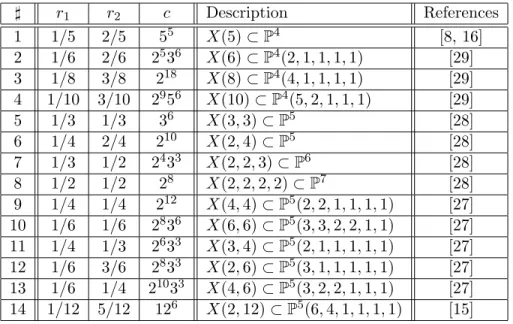
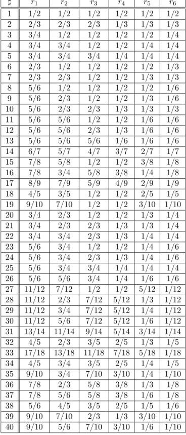
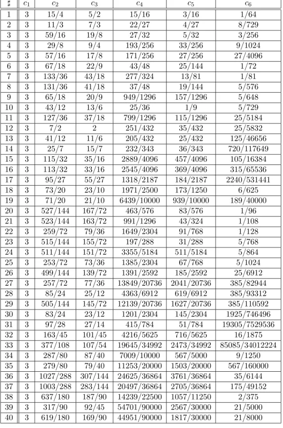
Appendix A. Here we provide several tables, which include information about Picard-Fuchs equation of Calabi-Yau manifolds.
Chapter 1
Historical Backgrounds
In this thesis we are going to introduce a special vector field on a moduli space of a family of Calabi-Yau manifolds. This vector field is in a close relationships with, and in a sense it is an extension of, the vector fields introduced by Darboux, Halphen and Ramanujan that we will review them below. Because of this relationship, the vector field is called Darboux-Halphen-Ramanujan, abbreviatly DHR,vector field. In this chapter, in§1.1 we explain the main problem in some special cases of low dimensions that have been done, and reformulate them in our language. Then in distinct sections §1.2, §1.3 and §1.4, resp., we review the works of Darboux, Halphen and Ramanujan, resp., that are in relationship with our main problem.
1.1
Problem Statement
To have an idea of DHR vector field, we explain the issue on a family of 1-dimensional Calabi-Yau manifolds, which are elliptic curves. For more details one can see [32] and [34].
Let E be an elliptic curve over C. We know that there are t1, t2, t3 ∈ C3, such that
∆ :=t32−27t236= 0, andE in Weirestrass form is considered as a following projective curve inP2,
E ={[x;y;z]∈P2|F(x, y, z) :=zy2−4(x−t1z)3+t2(x−t1z)z2+t3z3 = 0},
whereF(x, y, z) is the homogenization of the function
f(x, y) :=y2−4(x−t1)3+t2(x−t1) +t3,
that gives the following affine elliptic curve E0
E0 ={[x;y; 1]∈P2|f(x, y) = 0}.
Indeed ∆ is discriminant function of P(x) := 4(x−t1)3+t2(x−t1) +t3, and since ∆6= 0,
P and P′ do not vanish simultaneously. Also we can state
y2=P(x)⇒ 2ydy=P′(x)dx⇒ dx y = 2
dy P′(x).
So the 1-form dxy is holomorphic onE0. On the other hand, we know thatO := [0; 1; 0]∈E
is the only point at infinity andO /∈E0. So the one form xdxy is as well holomorphic onE0.
And if we letHdR1 (E0/C) be the first algebraic de Rham cohomology ofE0, then one can see
in [34, Proposition 2.2] that HdR1 (E0/C) is freely generated by [dxy ] and [xdxy ]. It is obvious
that E =E0\ {[0; 1; 0]}, so we have the inclusion ι :E0 → E. In [34, Proposition 2.4] we
can find that the inclusion ιinduces the isomorphism
ι∗ :HdR1 (E/C)→HdR1 (E0/C), (1.1)
hence there is a holomorphic 1-form α1 ∈ HdR1 (E/C) and a differential 1-form α2 ∈
HdR1 (E/C) such that ι∗(α1) = [dxy ] and ι∗(α2) = [xdxy ]. Since [dxy ] and [xdxy ] generate
H1
dR(E0/C), α1 and α2 as well generate HdR1 (E/C), so α1∧α2 6= 0. We can repeat this
history with another presentation ofE where
F(x, y, z) :=zy2−4(x−zt1)(x−zt2)(x−zt3),
f(x, y) =y2−4(x−t1)(x−t2)(x−t3),
with t1 6= t2 6= t3 (for more details see [34, § 3.5]). Because of isomorphism (1.1), in the
continue the necessary calculations attached toH1
dR(E/C), such as computation of
Gauss-Manin connection, will be done on the first de Rham cohomologyHdR1 (E0/C) of affine curve
E0.
Let E be an affine elliptic curve overCand
{0}=F2 ⊂F1 ⊂F0=HdR1 (E), dimC(Fi) = 2−i,
be the Hodge filtration of HdR1 (E) (see §2.3). For any αi ∈ Fi, i = 1,2, that satisfy the following intersection condition (see §2.6)
1 2πi
Z
E
α1∧α2= 1, (1.2)
there exist a unique
h= (h1, h2, h3)∈TH :={(t1, t2, t3)∈C3|t1 6=t2 6=t3}, (1.3)
such thatE is given by
9
inP2, and α1, α2, respectively, are given by dxy , xdxy , respectively. In factTH is the moduli
of (E, α1, α2, a1, a2, a3), where the ordered triple (a1, a2, a3) is the non-zero 2-torsion points
of E, i.e. 2ai = 0, i= 1,2,3. There is a unique vector field H, that we call it DHR vector field, on TH such that
∇H(dxy ) =−xdxy , ∇H(xdxy ) = 0, (1.5)
in which,∇ is the Gauss-Manin connection (see§2.5) defined on TH given by
∇
dxy
xdx y
=AH
dxy
xdx y
(1.6)
with
AH =
dh1
2(h1−h2)(h1−h3)
−h1 1
h2h3−h1(h2+h3) h1
+ dh2
2(h2−h1)(h2−h3)
−h2 1
h1h3−h2(h1+h3) h2
+ dh3
2(h3−h1)(h3−h2)
−h3 1
h1h2−h3(h1+h2) h3
.
The vector field H is given by
H = (h1(h2+h3)−h2h3)
∂ ∂h1
+ (h2(h1+h3)−h1h3)
∂ ∂h2
+ (h3(h1+h2)−h1h2)
∂ ∂h3
,
that can be seen as the following ordinary differential equation inC3:
H : ˙
h1 =h1(h2+h3)−h2h3
˙
h2 =h2(h1+h3)−h1h3
˙
h3 =h3(h1+h2)−h1h2
. (1.7)
So briefly, for the 1-forms α1 = dxy and α2 = xdxy that satisfy the following intersection
condition
(hαi, αji)1≤i,j≤2 =
0 1
−1 0
the DHR vector field H given by (1.7) satisfies the following equation,
∇Hα=
0 −1
0 0
α, (1.9)
in which α = α1 α2
t
, where t refers to matrix transpose. The system of differential
equation (1.7) appeared in the work of G. Darboux in 1978, and then G. Halphen (1881) and M. Brioschi (1881) contributed to the study of this differential equation system, that more details are presented in §1.2 and§1.3.
We can see the moduli of elliptic curves from another point of view and find another DHR vector field that is presented by Ramanujan’s system of differential equations. To see this, consider the triple (E, α1, α2), where E is an elliptic curve with two 1-forms α1 and
α2 satisfying (1.2). The moduli of (E, α1, α2)’s is given by
TR :={(t1, t2, t3)∈C3|27t23−t32= 0}, (1.10)
and more precisely for any (E, α1, α2) there exist a unique (r1, r2, r3)∈TR, such thatE is
given by
ER: y2= 4(x−r1)2−r2(x−r1)−r3, (1.11)
inP2, and α1 = dxy , α2 = xdxy . The Gauss-Manin connection of TR is given by the matrix
AR = ∆1
−32r1α− 1 12d∆
3 2α
∆r1−161r1d∆−(32r21+18r2)α 32r1α+121 d∆
,
∆ = 27r32−r23, α= 3r3dr2−2r2dr3,
and the intersection form matrix is given by (1.8). It is seen that there exist a unique vector field R on TR, which satisfies the following equation
∇Rα =
0 −1
0 0
α, (1.12)
and R is given by the Ramanujan’s system of differential equations
R :
˙
r1=r12−121r2
˙
r2= 4r1r2−6r3
˙
r3= 6r1r3−13r22
. (1.13)
It is natural to ask if there is any relationship between TH and TR, and the response is
positive. The algebraic morphismφ:TH→TR defined by
φ: (h1, h2, h3)7→(T,4
X
1≤i<j≤3
11
where
T := 1
3(h1+h2+h3),
connects two families. That is, if in ER we replace r with φ(h) we obtain the family EH,
and φmaps all related concepts ofEH, to the corresponding concepts ofER. In particular
φ∗H = R andφ∗AR =AH.
H. Movasati in [31, 33] worked on the family of mirror quintic 3-fold Calabi-Yau mani-folds and he found DHR vector field on a moduli space constructed on the family of mirror quintic 3-folds. We know that the family of quintic 3-folds are hypersurfaces of P4 given by homogeneous polynomials of degree 5. It is seen in [8] that the mirror of the quintic 3-folds are given by the family of Wψ’s defined as the variety obtained by a resolution of singularities of the following quotient:
Wψ :={[x0:x1:x2:x3:x4]∈P4|x50+x51+x52+x53+x54−5ψx0x1x2x3x4= 0}/G, (1.14)
whereG is the group
G:={(ζ1, ζ2,· · · , ζ5)|ζi5= 1, ζ1ζ2ζ3ζ4ζ5= 1},
acting in a canonical way and ψ5 6= 1 (for more details see Example 4.2). H. Movasati started to work with a special moduli spaces consisting of a Calabi-Yau manifolds and a basis of de Rham cohomology. More precisely, LetW1, W2be two mirror quintic 3-folds and
{αi1, α2i, αi3, α4i} be a basis of HdRn (Wi;C), i= 1,2. Then we have the following equivalence relation,
(W1,[α11, α21, α13, α14])∼(W2,[α21, α22, α23, α24]) (1.15)
if and only if there exist a biholomorphic function f : W1 → W2 such that f∗(α2j) =
αj1, j = 1,2,3,4. He considered T to be the moduli of pairs (W,[α1, α2, α3, α4]) under
above equivalence relation (1.15), where
αi ∈F4−i\F5−i, i= 1,2,3,4,
in whichF• is the Hodge filtration of HdR3 (W), satisfying the following intersection condi-tion,
(hαi, αji)1≤i,j≤4 = Φ.
with
Φ :=
0 0 0 1
0 0 1 0
0 −1 0 0
−1 0 0 0
. (1.16)
Theorem 1.1. Let T be the moduli of pairs(W,[α1, α2, α3, α4])defined above. Then there
is a unique vector fieldRa and a unique regular functiony on Tsuch that the Gauss-Manin
connection of the universal family of mirror quintic Calabi-Yau varieties over T composed
with the vector field Ra, namely ∇Ra, satisfies
∇Raα=
0 1 0 0
0 0 y 0
0 0 0 −1
0 0 0 0
α, (1.17)
in which
α= α1 α2 α3 α4
t
.
In fact,
T ∼={(t0, t1, t2, t3, t4, t5, t6)∈C7 |t5t4(t4−t50)6= 0}, (1.18) and under this isomorphism the vector field Ra as an ordinary differential equation is
Ra : ˙
t0 = t15(6·54t05+t0t3−54t4)
˙
t1 = t15(−58t60+ 55t40t1+ 58t0t4+t1t3)
˙
t2 = t15(−3·59t70−54t50t1+ 2·55t40t2+ 3·59t20t4+ 54t1t4+ 2t2t3)
˙
t3 = t15(−510t80−54t50t2+ 3·55t40t3+ 510t30t4+ 54t2t4+ 3t23)
˙
t4 = t15(56t40t4+ 5t3t4)
˙
t5 = t15(−54t50t6+ 3·55t40t5+ 2t3t5+ 54t4t6)
˙
t6 = t15(3·55t40t6−55t30t5−2t2t5+ 3t3t6)
, (1.19)
and y= 58(t4−t50)2 t3
5 is the Yukawa coupling.
1.2
Darboux
The system of differential equations
˙
t1+ ˙t2=t1t2
˙
t2+ ˙t3=t2t3
˙
t1+ ˙t3=t1t3
, (1.20)
first time appeared in 1878 in the works of Gaston Darboux (1842-1917) when he was studying the curvilinear coordinates and orthogonal systems in [12]. The problem that he was trying to prove is as follow: Let A and B be two fixed surfaces in the 3-dimensional Euclidean space R3 and suppose that Σ is the family of surfaces which are the locus of the points that the sum of their distances from the surfaces A and B are constant; and Σ′ is
13
from the surfaces A and B are constant. Is there a third family of surfaces that intersects
Σ andΣ′ orthogonally? This problem is equivalent to the following problem: Let A and B
be as before and suppose thatΣ is a family of surfaces parallel to A which is parameterized by v, and Σ′ is a family of surfaces parallel toB that is parameterized by w. Is there a third family of surfaces parameterized by u such that intersects Σ and Σ′ orthogonally? Note
that, two surfaces A1 and A2 are said to be parallel, if there exist a constant c such that
for anya1 ∈A1 anda2 ∈A2,d(a1, A2) =d(a2, A1) =c, in which drefers to the Euclidean
distance of R3; and we say that a family of surfaces is parameterized by s= s(x, y, z), if any surface belonging to this family is given by s(x, y, z) = constant, in which x, y, z are the standard coordinates ofR3. If for a function s=s(x, y, z), we define
sx= ∂s
∂x , sy = ∂s
∂y , sz= ∂s ∂z ,
then in the latter problem, the condition of parallelism is given by
vx2+v2y+vz2 = 1 & w2x+w2y+w2z = 1,
and the condition of orthogonality is given by
uxvx+uyvy+uzvz = 0 & uxwx+uywy+uzwz = 0.
So th problem is equivalent to the following system of equations,
v2
x+vy2+vz2= 1 wx2+w2y+wz2= 1 uxvx+uyvy +uzvz = 0 uxwx+uywy+uzwz= 0
. (1.21)
The more interesting case of this problem is when the family (u) is of second degree and Darboux proved that in this case this family is given by
x2
t1(u)
+ y
2
t2(u)
+ z
2
t3(u)
= 1,
in which t1, t2, t3 are functions ofu given by the following equation,
t3(
dt1
du + dt2
du) =t2( dt1
du + dt3
du) =t1( dt2
du + dt3
du). (1.22)
1.3
Halphen
In 1881, G. Halphen [23] studied the following system of differential equations
dt1 dz + dt2 dz =t1t2 dt2
dz + dtdz3 =t2t3 dt1
dz + dtdz3 =t1t3
, (1.23)
in whicht1, t2, t3 are three unknown variables. Halphen proved that this system satisfies an
important invariant property. To express this invariant property, for the constantsa, b, a′, b′, let
w = az+b
a′z+b′, (1.24)
ti = − 2a′
a′z+b′ +
ab′−ba′
(a′z+b′)2si, i= 1,2,3. (1.25)
Then by substituting (1.24) and (1.25) in the system (1.23), we have
ds1
dw +dsdw2 =s1s2 ds2
dw +dsdw3 =s2s3 ds1
dw +dsdw3 =s1s3
. (1.26)
Hence, the system (1.23) is invariant under the change of variables (1.24) and (1.25). So to find a general solution of (1.23), it is enough to first find a particular solution of (1.26), and then applying (1.25). Halphen expressed a solution of the system (1.23) in terms of the logarithmic derivatives of the null theta functions; namely,
t1 = 2(lnθ4(0|z))′,
t2 = 2(lnθ2(0|z))′, ′ =
∂ ∂z t3 = 2(lnθ3(0|z))′.
where
θ2(0|z) :=P∞n=−∞q
1 2(n+
1 2)2
θ3(0|z) :=P∞n=−∞q
1 2n2
θ4(0|z) :=P∞n=−∞(−1)nq
1 2n2
, q =e2πiz, z ∈H.
From it, we can found following three particular solutions of the system (1.23),
T1(z) = 8
ez+ 4e4z+ 9e9z+ 16e16z+. . . 1 + 2ez+ 2e4z+ 2e9z+ 2e16z+. . .,
T2(z) = 8 −
ez+ 4e4z−9e9z+ 16e16z−. . . 1−2ez+ 2e4z−2e9z+ 2e16z−. . .,
T3(z) =
15
And the general solution of (1.23), is given as
ti(z) =− 2a
′
a′z+b′ +
ab′−ba′ (a′z+b′)2Ti(
az+b
a′z+b′), i= 1,2,3.
In [5], Fr. Brioschi in 1881 studied the following extension of the system (1.23)
dt1 dz +
dt2
dz =t1t2+ϕ(z) dt2
dz +dtdz3 =t2t3+ϕ(z) dt1
dz +dtdz3 =t1t3+ϕ(z)
, (1.27)
in which, ϕ(z) is a function of z. Again Halphen in [21] introduced and studied a class of differential equations that the system (1.27) belongs to this class. In the case of three variables, he showed that this class is given by
dt1
dz =a1t21+ (λ−a1)(t1t2+t1t3−t2t3)
dt2
dz =a2t22+ (λ−a2)(t2t3+t2t1−t3t1)
dt3
dz =a3t23+ (λ−a3)(t3t1+t3t2−t1t2)
, (1.28)
where, a1, a2, a3, λ are constants. One can see that the system (1.28) is equivalent to the
system (1.23), when a1 = a2 = a3 = 0 and λ = 1. He proved that the system (1.28) also
satisfies the invariant property and it is in a direct relationship with the second order linear differential equations and he gave a solution of the system (1.28) in terms of hypergeometric functions X, Y, Z which had been introduced in [22].
1.4
Ramanujan
In this section we are going to find the origin of the system of equations (1.13) which has been done by Ramanujan in [37]. To do this, let
σr,s(n) =σr(0)σs(n) +σr(1)σs(n−1) +. . .+σr(n)σs(0),
in which, σν(n) = Pd|ndν and, by definition, σs(0) = 12ζ(−s), where ζ(s) is the Riemann Zeta-function. Ramanujan proves that
σr,s(n) =
Γ(r+ 1)Γ(s+ 1) Γ(r+s+ 2)
ζ(r+ 1)ζ(s+ 1)
ζ(r+s+ 2) σr+s+1(n)
+ζ(1−r) +ζ(1−s)
r+s nσr+s−1(n) +O{n
2/3(r+s+1)
To prove this equation Ramanujan encounters the following equations
P(q) = 1−24
∞
X
k=1
kqk 1−qk,
Q(q) = 1 + 240
∞
X
k=1
k3qk 1−qk,
R(q) = 1−504
∞
X
k=1
k5qk 1−qk,
that satisfy the following system of differential equations
qdPdq = P2(q)12−Q(q) qdQdq = P(q)Q(q3)−R(q) qdRdq = P(q)R(q2)−Q2(q)
. (1.29)
Next we give the relationships between the equations introduced by Ramanujan and Eisen-stein series. First note that, EisenEisen-stein seriesG2j of weight 2j, for integersj ≥2, are given as follow
G2j(τ) :=
X
m1,m2∈Z
(m1,m2)6=(0,0)
(m1τ +m2)−2j,
and working with the q-expansion of the Eisenstein series, the alternate notations of Eisen-stein series , for complexτ’s with Imτ >0, are defined
E2j(τ) :=
G2j(τ) 2ζ(2j) = 1−
4j B2j
∞
X
k=1
k2j−1e2πikτ 1−e2πikτ
= 1− 4j B2j
∞
X
r=1
σ2j−1(r)qr, q =e2πiτ, (1.30)
in which Bk’s are Bernoulli’s numbers. So E4(τ) = Q(q), E6(τ) =R(q), and also P(q) =
E2(τ), whereE2(τ) is defined by (1.30). Moreovere, if we let
(r1(τ), r2(τ), r3(τ)) = (2πi
12 E2(τ),12( 2πi
12)
2E
4(τ),8(2πi
12 )
3E 6(τ)),
then using the system (1.29), one easily finds that (r1, r2, r3) stisfy the following system of
differential equations
dr1
dτ =r12−121r2
dr2
dτ = 4r1r2−6r3 dr3
dτ = 6r1r3− 13r22
, (1.31)
Chapter 2
Hodge Theory and Families
In this chapter we briefly recall the basic facts related with Hodge theory. Firstly, in §2.1 the concept of integrable connections are stated. Secondly, in §2.2 the general theory of Hodge structure is provided. Then in§2.3 after introducing de Rham cohomology, as a nice example of Hodge structure, the Hodge decomposition of complexified de Rham cohomology and Hodge filtration is presented. Next in §2.4 the definitions and important results of families of complex manifolds are established. To provide a family of complex manifolds with a Hodge variation, one needs Gauss-Manin connection and Griffiths transversality that are stated in §2.5. Finally in §2.6 the concept of intersection forms is given. In particular we give a proof of the existence relationship between intersection forms and Hodge filtration in the context of de Rham cohomology.
In this chapter, a more detailed account as well as further information and omitted proofs to most of the results can be found in [13, 36, 41].
2.1
Local Systems and Integrable Connections
Definition 2.1. Let (X, o) be a pointed topological space andRbe a commutative ring with a unit. A local system of R-modules onX is defined to be a collectionV={Vx}x∈X of R-modules together with a collection of isomorphisms{ρ([γ])|Vx −→∼ Vy}x,y∈Xand [γ]∈π1(X,(x,y)), in whichπ1(X,(x, y)) is the homotopy classes of pathes fromx toy, that satisfy followings
(i) for the class of constant pathex atx,ρ([ex]) = idVx,
(ii) for any two classes [γ]∈π1(X,(x, y)) and [γ′]∈π1(X,(y, z)),ρ([γ∗γ′]) =ρ([γ′])◦ρ([γ]),
in which the compositionγ∗γ′ of pathesγ and γ′ means first traverse γ and then γ′,
both with double speed.
Usually we denote this local system by V, and moreover if R is a field and the fibers Vx are R-vector spaces, then the rank of V, which is denoted by rk(V), by definition is rk(V) := dimRVx. Also we denote aconstant system with fibersV on X by VX.
Definition 2.2. Let (X, o) be a pointed path-connected topological space. Then the col-lection {ρ([γ])|γ is a loop ato} defines the associatedmonodromy representation
ρ:π1(X, o)→GL(Vo).
The Definition 2.1 of a local system looks a little long and to make it more applicable we present an equivalent statement of it. To do this, we define alocally constant sheaf F on X to be a sheaf with the property that for some open cover {Ui}i∈I of X, the restrictions
ρUi,x :F(Ui) ˜→Fx, x ∈Ui are isomorphisms. Now suppose that X is path-connected and
locally simply-connected with a covering{Ui}i∈I of simply-connected open subsets of X. If
Vis a locally system onX, then the unique isomorphismsfx,y:Vx −→∼ Vy,x, y∈Ui, defined by any path connecting xtoy withinUi, give a locally constant sheaf by trivializations
φi:V|Ui ∼
−→VUi.
Conversely, letF be a locally constant sheaf onX. To associate a local systemVtoF, for any x∈X, let Vx be the stalkFx, and for any path γ : [a, b]→X, in which [a, b]⊂Ui for somei∈ I, define ρ(γ) =ρUi,b◦ρ
−1
Ui,a. In the case that [a, b] is not a subset ofUi, we divide
[a, b] to the subdivisions that any of them is a subset of some Ui and then define ρ(γ) as compositions of isomorphisms. Hence we have the following theorem:
Theorem 2.1. Let X be a path connected and locally simply-connected topological space. Then there is an one to one correspondence between local systems of R-modules and locally constant sheaves of R-modules.
From now on we substitute the topological space X with the complex manifold S and by a complex local system on S we mean a locally constant sheaf of C-vector space. If we denote the category of complex local systems on S by LocSysC(S), next we see that it is equivalent to the category of holomorphic vector bundles onS with an integral connection.
Definition 2.3. LetS be an n-dimensional complex manifold andV be anOS-module on it. A holomorphic connection ∇on V is a C-linear map∇: V → Ω1
S ⊗OS V, such that it
satisfies theLeibniz rule, i.e. for any local section f ofOS and any local sectionv of V,
∇(f v) =df⊗v+f∇(v). (2.1)
A local section v of V is said to be horizontal if ∇(v) = 0, and by notation V∇ denotes
Ker(∇).
Observation 2.1. If V is locally free of finite rank m, then by considering the frame {vj}mj=1 on an open subsetU of S, we can write ∇(vj) = Pmi=1Cijvi,and then define the
connection matrix as matrix of holomorphic 1-forms onU given byCU = (Cij)1≤i,j≤m. So for a holomorphic sectionv=Pmj=1gjvj, by applying the Leibniz’ rule we have
∇(v) = m
X
j=1
dgj⊗vj+ m
X
i,j=1
19
hence we can abbreviate the connection locally as follow
∇U =d+CU. (2.2)
By defining ΩpS(V) := ΩpS⊗OSV, the wedge product of differential forms induces
∇(p):ΩpS(V)→ΩpS+1(V) (2.3)
ω⊗v7→dω⊗v+ (−1)pω∧ ∇(v)
Definition 2.4. Thecurvature F∇ of connection ∇by definition is the map
F∇:V →Ω2S(V), (2.4)
F∇(v) =∇(1)◦ ∇(v).
The connection∇ is said to beflat orintegrable ifF∇= 0.
LetV be a holomorphic vector bundle onS of finite rankm. Then by using (2.2) we see thatF∇U =dCU−CU∧CU, in which (CU∧CU)ij =
Pm
k=1Cik∧Ckj. Thus the integrability
of∇is equivalent toCU∧CU =dCU. From now on, the pair (V,∇) refers to a holomorphic vector bundle V with integrable connection ∇ and we call it integrable connection on S. Integrable connections onS form a category that we denote it by IntCon(S).
If Vis a complex local system on S, then
V :=V⊗COS (2.5)
is a holomorphic vector bundle onS. By defining∇(v⊗f) =df⊗v, for any local sectionsf and v, resp., ofOS and V, resp., we can see that ∇is an integrable connection ofV, hence (V,∇) is an integrable connection. Conversely, let (V,∇) be an integrable connection. Then by definingV:= V∇, it is seen thatV is a complex local system on S and (V,∇)≃
V⊗C(OS, d) (for more details see [36,§ 10.3]). So we have the following theorem:
Theorem 2.2. Let S be a complex manifold. Then LocSysC(S)∼= IntCon(S).
2.2
Hodge Structure
Definition 2.5. LetV be aZ-module of finite rank andVC:=V⊗ZCits complexification.
A Hodge structure of weight kon V is a direct sum decompositio
VC=
M
p+q=k
Vp,q, (Hodge decomposition) (2.6)
The Hodge filtration of V associated to the Hodge structure (2.6) is given by
Fp(V) =M r≥p
Vr,k−r. (2.7)
To simplify the notation, we write Fp instead of Fp(V) when no confusion arise. So obvi-ously we have the decreasing filtration
0 =Fk+1 ⊂Fk⊂. . .⊂F1 ⊂F0 =VC. (2.8)
Also one can seeVp,q=Fp∩Fq andV
C=Fp⊕Fk−p+1 (or equivalentlyFp∩Fk−p+1 = 0).
Conversely, the decreasing filtration (2.8) of VC with the propertyVC=Fp⊕Fk−p+1 gives
a Hodge filtration of weightk by definingVp,q =Fp∩Fq.
Definition 2.6. Let S be a complex manifold. A variation of Hodge structure of weight
k on S is a quadruple (S,V,∇,F•), in which V is a local system of finitely generated abelian groups on S, ∇: V → V ⊗Os ΩS1 is an integrable connection and F• := {Fp} is a finite decreasing filtration of the holomorphic vector bundle V :=V⊗ZOS by holomorphic subbundles (theHodge filtration), such that following conditions hold:
(i) for each s∈ S the filtration {Fp(s)} of V(s) ≃ V
s⊗ZC defines a Hodge structure of
weight kon the finitely generated abelian group Vs,
(ii) the connection ∇, whose sheaf of horizontal sections is VC, satisfies the Griffiths’ transversality condition
∇(Fp)⊂Ω1S⊗ Fp−1. (2.9)
Note that in all the concepts of this section we can substitute the group of integersZby the group of realsR, and have thereal Hodge structure orreal variation of Hodge structure.
2.3
de Rham Cohomology and Hodge Filtration
LetX be an n-dimensional differentiable manifold,TX the tangent bundle ofX and T∗X
its cotangent bundle. By definition let
EXm := Γ (X,ΛmT∗X), m= 1,2,3, . . .
be the bundle of differentialm-forms; note that by the space of 0-forms we mean the space of differentiable functions. Then by considering the long exact sequence
EX• : 0 d − → EX0
d − → EX1
d −
→. . .−→ Ed Xn−1 d − → EXn
d − →0,
in whichd is exterior derivative, we define theq-th de Rham cohomology HdRq (X) of X as follow,
HdRq (X) :=Hq(EX•, d) =
KerEXq d − → EXq+1
ImEXq−1 −→ Ed Xq
21
We can also see de Rham cohomology in the point of view of ˇCech cohomology. To do this let Ωq(X),q = 1,2, . . . ,be the sheaf of differential q-forms, and Ω0(X) :=O(X) the sheaf
of differential functions on X. Then we have the de Rham complex
Ω•(X) : 0→RX ֒→Ω0(X)−→d Ω1(X)−→d . . .−→d Ωn−1(X)→−d Ωn(X)−→d 0,
in which RX is a constant sheaf on X. If X is compact, then we have the following isomorphism
HdRq (X)∼= ˇHq(X,R).
Also in the context of singular cohomology, by de Rham lemma one has the following isomorphism
HdRq (X)∼=Hq(X,R), (de Rham lemma). (2.11) Note that ifX is connected, then for q= 0 we have
HdR0 (X)∼={locally constantR-valued functions onX} ∼=R. (2.12) Next we suppose that X is a complex n-dimensional manifold, and hence m = 2n dimensional differential manifold. Let J be the complex structure of X. Then for any p ∈ X, complexify TpX to obtain (TpX)C := TpX ⊗RC which is a complex vector space
isometric toC2n. The automorphismJp :TpX→ TpXextends naturally to a automorphism Jp : (TpX)C→(TpX)C, which is linear overC. SinceJp2 =−id, the eigenvalues ofJp are±i, wherei=√−1. LetTp(1,0)X andTp(0,1)X, resp., be the eigenspaces of Jp corresponding to eigenvalues iand −i, resp. Then we see that Tp(1,0)X∼=Cn∼=Tp(0,1)X and that (TpX)C=
Tp(1,0)X⊕ Tp(0,1)X. As this is valid for every point p∈X, we have defined two subbundles of (TX)C:= TX⊗RCsuch that (TX)C =T(1,0)X⊕ T(0,1)X. By a similar argument we
can see that the complexified cotangent bundle (T∗X)
C := T∗X⊗RC splits into pieces
(T∗X)C = T∗(1,0)X⊕ T∗(0,1)X. If we define Λp,qX := ΛpT∗(1,0)X⊗ΛqT∗(0,1)X, then by
using of splitting of (T∗X)
C it follows that
ΛkT∗X⊗RC= k
M
j=0
Λj,k−jX.
This is decomposition of the exteriork-forms onX induced by the complex structureJ. A section of Λp,qX is called a (p, q)-form and by notation we write
EXp,q:= Γ(X,Λp,qX).
Now we define ∂ and ¯∂ to be the components of exterior derivativedas follow, ∂:EXp,q→ EXp+1,q & ∂¯:EXp,q→ EXp,q+1.
Then∂ and ¯∂ are first-order partial differential operators on complexk-forms which satisfy d=∂+ ¯∂. The identityd2 = 0 implies that∂2= ¯∂2 = 0 and∂∂¯+ ¯∂∂= 0. So by using the differential operator ¯∂ we have the following long exact sequence
EXp,•: 0→ E p,0
X
¯
∂ −→ EXp,1
¯
∂
and hence we define the (p, q)-th Dolbeault cohomology Hp,q as follow
Hp,q(X) :=Hq(Ep,•,∂) =¯ Ker
EXp,q
¯
∂ − → EXp,q+1
Im
EXp,q−1
¯
∂ −→ EXp,q
.
If we denote the sheaf of holomorphic p-forms by ΩpX and the sheaf of (p, q)-forms by Ωp,qX , then we consider theDolbeault complex as follow
ΩXp,• : 0→ΩpX ֒→ΩXp,0 −→∂¯ Ωp,X1 −→∂¯ . . .−→∂¯ Ωp,qX −→∂¯ Ωp,qX +1−→∂¯ . . . , p= 0,1,2, . . .
which is a resolution of ΩpX, and byDolbeault’s theorem we have the following isomorphism
Hp,q(X)∼=Hq(X,ΩpX), (Dolbeault’s theorem). (2.13)
Next we are going to introduce a real Hodge structure of weight k on Hk
dR(X). To do
this we need X to be a K¨ahler manifold. By definition, a K¨ahler manifold is a 4-tuple (X, ω, g, J), in which (X, ω) is a symplectic manifold, i.e. ω is a non-degenerate closed 2-form onX, with the complex structureJ and the Riemannian metric gsuch that for any two vector fields v, w on X we have g(v, w) =ω(v, Jw). Hence one can easily see that
h:=g+iω (2.14)
is a hermitian metric on X. As we saw in (2.6), we also need to complexify Hk
dR(X) and
we denote its complexification as follow
HdRk (X;C) :=HdRk (X)⊗RC,
and by de Rham lemma (2.11) we have
HdRk (X;C)∼=Hk(X,C). (2.15)
Following theorem gives the real Hodge structure that we desire(see [36, Theorem 1.8]).
Theorem 2.3. (Hodge Decomposition Theorem) IfX is a compact K¨ahler manifold, then we have
HdRk (X;C) = M p+q=k
Hp,q(X), (2.16)
and moreover,Hp,q(X) =Hq,p(X), in which ”¯.” refers to complex conjugation.
Hence the complex conjugation map implies the isomorphism
Hp,q(X)∼=Hq,p(X), (2.17)
thus if we denote the Hodge numbers byhp,q(X) := dim
CHp,q(X), thenhp,q(X) =hq,p(X).
23
hp,q = hn−q,n−p; to see this first we need to know a little about the Hodge ∗-operator. The K¨ahler metricg ofX present an inner product onTxX, and hence it induces an inner product on T∗
xX and on the wedge product of Tx∗X, i.e. the bundle of q-forms ΛqTx∗X, which we denote it also byg. Using gwe can define the positive definite hermitian formgC x on (TxX)C, for any x∈X, as follow
gCx(v⊗λ, w⊗µ) = (λ¯µ)gx(v, w), ∀λ, µ∈Cand andv, w∈ TxX. (2.18)
Definition 2.7. TheHodge ∗-operator
∗: ΛqT∗X→Λ2n−qT∗X, (2.19)
in any point x∈X is defined by
α∧ ∗β =gx(α, β)volg(x), ∀α, β ∈ΛqTx∗X, (2.20)
in which volg(x) refers to the volume form ofX with respect to the metricginx, of course with a fixed orientation onX.
The Hodge ∗-operator (2.19) C-linearly extends to the operator
∗: Λq(T∗X)C→Λ2n−q(T∗X)C, (2.21)
that is induced by
α∧ ∗β¯=gCx(α, β)volg(x), ∀α, β ∈ΛqTx∗X, (2.22) in which gC
x(., .) is given by (2.18). The operator given in (2.21) is also called Hodge ∗ -operator and it is not difficult to see that it sends Λp,qX to Λn−q,n−pX (for more details one refers to [24]). And finally the equalityhp,q=hn−q,n−p, follows from following theorem which is proved in [24, Corollary 3.3.14].
Theorem 2.4. The Hodge ∗-operator on a compact K¨ahler manifold X, induces the fol-lowing isomorphism,
Hp,q(X)∼=Hn−q,n−p(X).
Notation 2.1. For a compact K¨ahler manifoldX, we denote bybk(X) := dimCHdRk (X;C)
which is known ask-th Betti number ofX. And if there is no ambiguity about the manifold X, we just denote it bybk.
We can summarize above facts in the following lemma.
Lemma 2.1. Let X be a compact K¨ahler manifold of complex dimension n. Then the followings hold:
(i) bk= P p+q=k
hp,q, 0≤k≤2n.
(iii) hp,q=hn−q,n−p, 0≤p, q≤n.
By using Lemma 2.1, we consider the Hodge diamond of an n-dimensional compact K¨ahler manifoldX as follow
Lemma 2.1(ii)
←→
h0,0
h1,0 h1,0
h2,0 h1,1 h2,0
. .. . ..
hn−1,0 hn−2,1 . . . hn−2,1 hn−1,0
Lemma 2.1(i)
−−−−−−−−→ hn,0 hn−1,1 . . . hn−1,1 hn,0 lLemma 2.1(iii) (2.23)
hn−1,0 hn−2,1 . . . hn−2,1 hn−1,0
. .. . ..
h2,0 h1,1 h2,0
h1,0 h1,0
h0,0
Now, as we saw in (2.7), we present the Hodge filtration of HdRk (X), 0 ≤ k ≤ n, as follow
Fp(X) = M p≤r≤k
Hr,k−r(X), 0≤p≤k, (2.24)
and hence we have the following decreasing filtration
F•: 0 =Fk+1⊂Fk⊂. . .⊂F1 ⊂F0 =HdRk (X;C). (2.25) One can easily see the following lemma.
Lemma 2.2. Following hold for the Hodge filtration F• of Hk
dR(X):
(i) Hp,q=Fp∩Fq, 0≤p, q≤k.
(ii) Hk
25
2.4
Families and Complex Deformations
Definition 2.8. By afamily of complex manifolds we mean a holomorphic proper submer-sion π :X → S, in which X and S are complex manifolds. The manifold S sometimes is called thebase manifold and in the case that there is no ambiguity about the base manifold, we simply denote the family of complex manifolds byX.
For anys∈S, letXsbe the fiber ofπ over the points, i.e. Xs:=π−1(s). IfS is connected and o∈S is a base point, then we say that X is a family of deformations of the fiberXo, and any fiber Xs, s ∈ S, is said a complex deformation of Xo. An infinitesimal complex
deformation of X is a deformation with base space S := Spec(C[ǫ]). Following theorem gives a representation of infinitesimal deformation ofX (see [18, Theorem 22.1]).
Theorem 2.5. The isomorphism classes of infinitesimal deformations of a compact complex manifold X are parametrized by elements in H1(X,TX).
Remark 2.1. LetXbe ann-dimensional compact complex manifold. The space of complex deformations of X sometimes is called complex moduli space of X which is denoted by Mcmplx(X). IfE is a holomorphic vector bundle onX, thenSerre duality states that
Hq(X, E)∼=Hn−q(X, KX⊗E∗)∗,
in which KX = Λn,0X is the canonical bundle ofX. So by Theorem 2.5, we have
Mcmplx(X)∼=Hn−1(X, KX ⊗ T∗X)∗. (2.26)
Next we state the well known Ehresmann Lemma, and then by applying it to the family of complex manifolds we conclude a trivialization of them.
Theorem 2.6. (Ehresmann Lemma) Let π:X →S be a proper smooth submersion of differentiable manifolds over a contractible pointed base (S, o). Then there exists a diffeo-morphism T = (T1, T2) :X −→∼ Xo×S, such that T2 =π.
Hence the first component of trivialization T, i.e. T1 : X → Xo, induces a diffeomor-phismXs∼=Xo, for any s∈S.
Now in [41, Proposition 9.5] we have the following theorem.
Theorem 2.7. Let π:X →S be a family of complex manifolds over a pointed base (S, o). Then up to replacingS by a neighborhood of the base pointo, there exists aC∞trivialization
T = (T1, π) :X →Xo×S, such that the fibers of T1 are complex submanifolds ofX.
Note that in the complex case the trivialization T, in general, is not holomorphic, but the diffeomorphismesT1 :Xs−→∼ Xo, s∈S, enable us to verify that the family of complex structures onXo parameterized byS, i.e. Xs’s, varies holomorphically with s∈S.
Proposition 2.1. [41, Propositions 9.20 and 9.21] Let π :X →S be a family of complex manifolds that Xo is a K¨ahler manifold. Then for any s∈S, close enough to o, following
hold:
(i) hp,q(Xs) =hp,q(Xo), for suitable p and q’s.
(ii) Hk
dR(Xs;C) =
L
p+q=k
Hp,q(X s).
Theorem 2.8. [41, Theorem 9.23]Let π :X →S be a family of complex manifolds. If Xo
is a K¨ahler manifold, then for any s∈S, close enough to o, Xs is also a K¨ahler manifold.
Definition 2.9. By a family of K¨ahler manifolds we mean a family of complex manifolds X over the pointed base (S, o) that any fiber Xs,s∈S, is a K¨ahler manifold.
Remark 2.2. (i) Considering Theorem 2.8, in the family of complex manifoldsX, up to a neighborhood of base point o, to have a family of K¨ahler manifolds it is enough that the fiber Xo be a K¨ahler manifold.
(ii) Note that in the family of complex manifolds X any fiber Xs is a compact complex manifold, and to further emphasize sometimes we use thefamily of compact complex
(K¨ahler) manifolds instead of the family of complex (K¨ahler) manifolds.
(iii) Under hypothesis of Proposition 2.1, for any s ∈S near too, bk(Xs) = bk(Xo), and (2.24) gives the following decreasing Hodge filtration of HdRk (Xs;C)
0 =Fk+1(Xs)⊂Fk(Xs)⊂. . .⊂F1(Xs)⊂F0(Xs) =HdRk (Xs;C). (2.27) And also dimCFj(Xs) = dimCFj(Xo), 0≤j≤k+ 1.
2.5
Gauss-Manin Connection and Griffiths Transversality
Letπ :X →S be a family of compact K¨ahler manifolds. In this section first we are going to introduce a locally constant sheaf onS and then after presenting an integrable connection, which is known asGauss-Manin connection, we conclude a real variation of Hodge structure on S.
Let VX be a constant sheaf on X for some group V, for example V = C,Q,R or Z.
Then consider the sheaf Rkπ
∗VX on S, in which Rkπ∗ refers to k-th derived functor of
the pushforward (to know more about the derived functor one can see [36, § A.2.4]). By [13, Corollary 2.25] we have the following more understandable presentation of the stalks (Rkπ
∗VX)s:
Theorem 2.9. For any s∈S, one has the following isomorphism
27
In particular, in the case that V =C, we have (Rkπ∗CX)s≃Hk(Xs,C)
(2.15)
≃ HdRk (Xs;C), hence Rkπ
∗CX is a locally constant sheaf on S. Formally speaking, Rkπ∗CX is the sheaf
associated to the presheaf U 7→Hk(π−1(U),C). In fact, for a contractible open subsetU ⊂ S, by Ehresmann Lemmaπ−1(U)∼=U×Xsfor somes∈S, soHk(π−1(U),C)≃Hk(Xs,C). Thus (Rkπ
∗CX)|U is just the constant sheaf with group HdRk (Xs;C). Hence, by Theorem 2.1, equivalently we can consider Rkπ∗CX as a local system on S. Next by following the
process of constructing holomorphic vector bundle (2.5) from a local system, we define
HdRk (X/S) :=Rkπ∗CX ⊗COS, (2.28) which is a holomorphic vector bundle onS, so by Theorem 2.2 there exist a unique integrable connection onHdRk (X/S) such that the space of its horizontal local section isRkπ∗CX. And
also, with a little neglect, we have
HdRk (X/S)s ∼=HdRk (Xs;C). (2.29) For more details one refers to [36, Prop-Def 10.24].
Definition 2.10. The holomorphic vector bundleHdRk (X/S) defined in (2.28) is calledk-th relative de Rham cohomology group and the unique integrable connection
∇GM:HdRk (X/S)→Ω1S⊗OSH
k
dR(X/S),
is saidGauss-Manin connection.
For a vector field v on S, consider the map
v⊗Id : Ω1S⊗OS H
k
dR(X/S)→HdRk (X/S),
then by composing the Gauss-Manin connection∇GM
withv⊗Id we define
∇GMv :HdRk (X/S)→HdRk (X/S) (2.30)
∇GMv = (v⊗Id)◦ ∇
GM
.
From now on, if there is no danger of confusion we denote the Gauss-Manin connection by ∇instead of∇GM
.
Observation 2.2. Proposition 2.1 implies that the k-th relative de Rham cohomology group HdRk (X/S) is local free of finite rank, say m. By considering the locally frame ̟ := {ωj}mj=1, the same as Observation 2.1, we have the Gauss-Manin matrix connection
which is denoted by GM̟. More precisely if we consider the matrix presentation of ̟,
which we denote it also by ̟, as follow
in which trefers to the matrix transpose, then
∇̟:= (∇ω1 ∇ω2 . . . ∇ωm)t=GM̟⊗̟.
Note that for any s∈S and anyj∈ {1,2, . . . , m},ωj(s)∈HdRk (Xs;C) and we can present it by a k-form inXs that we denote it also byωj(s).
Considering Remark 2.2(iii), each fiber of HdRk (X/S) has a Hodge filtration, and this yields a decreasing filtration of HdRk (X/S) by holomorphic subbundles
F• : 0 =Fk+1⊂ Fk⊂. . .⊂ F1⊂ F0 =HdRk (X/S), (2.31)
such that for anys∈S and any p∈ {0,1,2, . . . , k},
Fsp ∼=Fp(Xs) =
M
p≤r≤k
Hr,k−r(Xs).
By definition, the filtration F• given in (2.31) is called Hodge filtration of Hk
dR(X/S).
However, one can still define the bundles Hp,n−p = Fp/Fp+1 such that for any s ∈ S,
Hp,ns −p ∼= Hp,n−p(Xs). And now to complete the real Hodge variation of S that we are looking for, it is enough to show the Griffiths’ transversality which is given in the following theorem (see [18, Theorem 16.4]).
Theorem 2.10. (Griffiths’ transversality) Let π : X → S be a family of compact K¨ahler manifolds and HdRk (X/S) be its k-th relative de Rham cohomology group. If ∇ is the Gauss-Manin connection and F• is the Hodge filtration of HdRk (X/S) given in (2.31), then
∇Fp ⊂Ω1S⊗ Fp−1, p= 1,2, . . . k.
2.6
Intersection Forms
In this section, we suppose thatX is the familyπ :X →Sofn-dimensional compact K¨ahler manifolds. For any α, ω∈HdRn (X/S), theintersection form ofα and ω by definition is
hα, ωi(s) := Tr(α(s)`ω(s)), ∀s∈S,
in which ”`” refers to the cup product. But in de Rham cohomology, the cup product of differential forms is induced by the wedge product, hence in the family X and its relative de Rham cohomology group defined by differential forms, the intersection form is defined as
hα, ωi(s) =
Z
Xs
α(s)∧ω(s). (2.32)
29
For a fixed s∈ S, we know that Xs is an n-dimensional compact K¨ahler manifold. It is obvious that if η, ν ∈Hn
dR(Xs;C), thenη∧ν = (−1)n(ν ∧η), thus hη, νi= (−1)nhν, ηi.
Also it is easy to see that
η∧ν = 0, for any η∈Fi(Xs) , ν ∈Fj(Xs) withi+j≥n+ 1, (2.33)
in which F•(X
s) is the Hodge filtration of HdRn (Xs;C). To show this, first suppose that (x1, x2, . . . , xn,x¯1,x¯2, . . . ,x¯n) is a local chart of Xs, so since Fi(Xs) = L
i≤r≤n
Hr,n−r(Xs),η is presented in this chart as follow
η= X
♯Iη≥i
♯Jη≤n−i
fIηJηdxIηd¯xJη,
and similarly ν∈Fj(X
s) is locally presented as follow
ν = X
♯Iν≥j
♯Jν≤n−j
gIνJνdxIνd¯xJν,
thus,
η∧ν= X
♯Iη≥i, ♯Jη≤n−i
♯Iν≥j, ♯Jν≤n−j
hIηJηIνJνdxIηdxIνd¯xJηd¯xJν.
Now we know that ♯Iη+♯Iν ≥i+j ≥n+ 1, hence dxIηdxIν = 0, and this completes the
proof of (2.33). So we can state the following lemma.
Lemma 2.3. LetX be a family ofn-dimensional compact K¨ahler manifolds. Then following hold:
(i) hα, ωi= (−1)nhω, αi, for anyα, ω∈HdRn (X/S).
(ii) If F• is the Hodge filtration of Hn
dR(X/S), then
hFi,Fji= 0, for i+j≥n+ 1. (2.34)
Notation 2.2. Let X be the family of n-dimensional compact K¨ahler manifolds over the pointed base (S, o). By dimHdRj (X/S) =lwe mean that dimCHdRj (Xo;C) =l. Proposition 2.1 guaranties that, up to a neighborhood of o, for any s∈S, dimCHdRj (Xs;C) =l. Also by dimFj =kwe mean that dim
CFj(Xs) =k, for any s∈S.
Remark 2.3. We are going to consider a special case with respect to the dimension of de Rham cohomology. Let X be the family of n-dimensional compact K¨ahler manifolds such that dimHn
dR(X/S) =n+ 1. Also suppose that dimFi = (n+ 1)−i, i= 0,1, . . . , n, where
F• is the Hodge filtration ofHn
dimHp,q(Xs) = 1 if p+q =n. So if we consider a local frame {ωi}ni=1+1 of HdRn (X/S) with
ωi ∈ F(n+1)−i, then we can define the matrix of intersection forms as follow
Ω = (Ωij)1≤i,j≤n+1 := (hωi, ωji)1≤i,j≤n+1.
By using of Lemma 2.3, in the case that nis an odd integer Ω is given as
Ω =
0 0 . . . 0 Ω1(n+1)
0 0 . . . Ω2n Ω2(n+1)
..
. ... . .. ... ...
0 −Ω2n . . . 0 Ωn(n+1)
−Ω1(n+1) −Ω2(n+1) . . . −Ωn(n+1) 0
, (2.35)
and in the case thatnis an even integer Ω is presented as follow
Ω =
0 0 . . . 0 Ω1(n+1)
0 0 . . . Ω2n Ω2(n+1)
..
. ...
. .. Ωll . ..
..
. ...
0 Ω2n . . . Ωnn Ωn(n+1)
Ω1(n+1) Ω2(n+1) . . . Ωn(n+1) Ω(n+1)(n+1)
, (2.36)
Chapter 3
Picard-Fuchs Equation as a
Self-Dual Linear Differential
Equation
In the pervious chapter we introduced the Gauss-Manin connection. We saw that the composition of Gauss-Manin connection with a vector field yields a differential operator on the relative de Rham cohomology group of a family of complex manifolds. In this chapter we are going to study this operator and its generated linear differential equations. First in§3.1, we briefly state some basic facts related with differential operators. We give an algorithm to find the relationships among coefficients of a self-dual linear differential operator of an arbitrary degree. Next in §3.2, a special linear differential operator associated with a holomorphicn-form, which is called Picard-Fuchs equation, is presented. At the end of this chapter, in§3.3, after fixing some certain hypothesis on a family of complex manifolds, we prove that its relative de Rham cohomology group has a special type of frame, which we call it Yukawa frame. To do this we use the properties of coupling function that we prove them in Proposition 3.3 in context of de Rham cohomology. Also in Proposition 3.4, we give a relationship between the dimensions of the relative de Rham cohomology group and its Hodg filtration, which weakens our primary hypothesis.
The basic concepts of this chapter are discussed more detailed in [2, 3].
3.1
Differential Operators
In this section by R we mean a simple commutative differential ring, with quotient field k and derivative (.)′, and R[∂] is the ring of differential operators. We assume that the ring of constantsC is an algebraically closed field of characteristic zero, such thatkalso has the same field of constants C and k6=C.
In this section, for more details and proofs, one refers to [3].
Definition 3.1. A differential R-module is a pair (M, ∂), where M is a finitely generated R-module and∂:M →M is a map satisfying