CONSTRAINT REASONING FOR DIFFERENTIAL MODELS

CONSTRAINT REASONING FOR DIFFERENTIAL MODELS

Dissertação apresentada para obtenção do Grau de Doutor em Engenharia Informática pela Universidade Nova de Lisboa, Faculdade de Ciências e Tecnologia.

iii

Teresa and Filipe

v I am specially indebted to Pedro Barahona who supported me, not only as the supervisor of this work, but also in all my academic formation. He is an excellent supervisor which I greatly recommend to any one intending to start a PhD in constraint programming. He has the rare ability of being open minded with respect to new ideas and contribute diligently to their success. Despite his overbooked schedule, he was always present whenever needed. He is a good friend and is a pleasure to work with him.

I am very grateful to Frédéric Benhamou and all his research team for their good hospitality and their crucial support in the early phases of this work. Thanks to Frédéric Goualard and Laurent Granvilliers for their friendship and all our valuable discussions.

Special thanks to Luís Moniz Pereira, for his careful reading and comments on the introduction and conclusions of this work, but above all, for his excellent work in promoting Artificial Intelligence which attracted me in the first place for taking a computer science degree.

My acknowledgements to the Computer Science Department for having conceded me three sabbatical years which were extremely important for the progress of this work.

Many thanks to my colleagues in the Computer Science Department and CENTRIA for their companionship, trust and concern. In particular, I am grateful to the constraint research group for creating a stimulating working environment. Thanks to my good friends Anabela and Cecília for their sincere care and help, promptly sharing with me their own resources whenever I needed.

Thanks to all my family for their love and precious help in handling so many practical problems which allowed me to fully concentrate on my work. I am particularly grateful to my parents for their continuous support and belief on my own choices.

vii A motivação básica deste trabalho foi a integração de modelos biofísicos na tecnologia de restrições com intervalos para o apoio à decisão. Comparando as características mais importantes dos modelos biofísicos com o poder de representação das restrições com intervalos, foi fácil de identificar que a maior insuficiência estava relacionada com a representação de equações diferenciais. A dinâmica dos sistemas é frequentemente modelada por equações diferenciais, mas não era possível representar uma equação diferencial como uma restrição que possa ser incluída num modelo de restrições.

Consequentemente, o objectivo principal deste trabalho é a integração de equações diferenciais ordinárias na tecnologia de restrições com intervalos. Neste trabalho é alargado o âmbito das restrições com intervalos com um novo formalismo para o tratamento de equações diferenciais como Problemas de Satisfação de Restrições Diferenciais. Este paradigma permite a especificação de equações diferenciais ordinárias juntamente com informação relacionada através de restrições, e proporciona técnicas de propagação eficientes para a redução do domínio das suas variáveis. Assim, toda esta informação é integrada numa única restrição cujas variáveis podem ser usadas noutras restrições do modelo. O método usado para reduzir os domínios destas variáveis pode ser então combinado com os métodos de redução associados às outras restrições num algoritmo de propagação geral para diminuir a incerteza de todas as variáveis do modelo.

A utilização de um algoritmo de propagação de restrições para a redução dos domínios das variáveis, isto é, a imposição de consistência local, revelou-se insuficiente para o apoio à decisão em problemas práticos que envolvam equações diferenciais. A redução dos domínios não é, em geral, suficiente para permitir decisões seguras e a principal razão deriva da não linearidade das equações diferenciais. Consequentemente, um objectivo complementar deste trabalho é a proposta de um novo critério de consistência particularmente apropriado ao apoio à decisão com modelos diferenciais, isto é, que apresente um equilíbrio adequado entre a redução dos domínios obtida e o respectivo esforço computacional. Vários algoritmos alternativos foram propostos para impor este critério, tendo sido feito um esforço no sentido de conceber implementações capazes de fornecer resultados a qualquer momento da execução.

Uma vez que o critério de consistência depende da existência de soluções canónicas, é proposto um mecanismo de pesquisa local que pode ser integrado com a propagação de restrições e, em particular, com os algoritmos de imposição do critério para antecipar a descoberta de soluções canónicas.

ix The basic motivation of this work was the integration of biophysical models within the interval constraints framework for decision support. Comparing the major features of biophysical models with the expressive power of the existing interval constraints framework, it was clear that the most important inadequacy was related with the representation of differential equations. System dynamics is often modelled through differential equations but there was no way of expressing a differential equation as a constraint and integrate it within the constraints framework.

Consequently, the goal of this work is focussed on the integration of ordinary differential equations within the interval constraints framework, which for this purpose is extended with the new formalism of Constraint Satisfaction Differential Problems. Such framework allows the specification of ordinary differential equations, together with related information, by means of constraints, and provides efficient propagation techniques for pruning the domains of their variables. This enabled the integration of all such information in a single constraint whose variables may subsequently be used in other constraints of the model. The specific method used for pruning its variable domains can then be combined with the pruning methods associated with the other constraints in an overall propagation algorithm for reducing the bounds of all model variables.

The application of the constraint propagation algorithm for pruning the variable domains, that is, the enforcement of local-consistency, turned out to be insufficient to support decision in practical problems that include differential equations. The domain pruning achieved is not, in general, sufficient to allow safe decisions and the main reason derives from the non-linearity of the differential equations. Consequently, a complementary goal of this work proposes a new strong consistency criterion, Global Hull-consistency, particularly suited to decision support with differential models, by presenting an adequate trade-of between domain pruning and computational effort. Several alternative algorithms are proposed for enforcing Global Hull-consistency and, due to their complexity, an effort was made to provide implementations able to supply any-time pruning results.

Since the consistency criterion is dependent on the existence of canonical solutions, it is proposed a local search approach that can be integrated with constraint propagation in continuous domains and, in particular, with the enforcing algorithms for anticipating the finding of canonical solutions.

xi LOGIC

¬ The negation operator

∧ The conjunction operator

∨ The disjunction operator

⇒ The implication operator

∀ The universal quantifier

∃ The existential quantifier

SET THEORY

∈ An element of

∉ Not an element of

⊆ A subset of

⊂ A proper subset of

∩ The intersection operator

∪ The union operator

⊎ The union hull operator

∅ The empty set

REAL VALUES, INTERVALS AND BOXES r, ri, k A real value

a, b, c, d A real value representing the bound or the center (c) of an interval r The largest F-number not greater than r

r The smallest F-number not lower than r -∞, +∞ The minus and the plus infinity F-numbers I, Ii. K An interval, either a real interval or an F-interval

IR, IRi A real interval

IF, IFi An F-interval

<a..b> An interval bounded by a and b (closed, half closed or open) [a..b] A closed interval bounded by a and b

xii

(a..b), (-∞..+∞) An open interval

[a..a], [a], {a} A degenerate interval with the singe real value a B, Bi A box, either an R-box or an F-box

<I1,...,In> A box with n intervals

<IR1,...,IRn> A real box with n real intervals <IF1,...,IFn> An F-box with n F-intervals

INTERVAL BASIC FUNCTIONS AND APPROXIMATIONS

left([a..b]) The function that returns the left bound of [a..b] right([a..b]) The function that returns the right bound of [a..b] center([a..b]) The function that returns the mid value of [a..b] width([a..b]) The function that returns the width of [a..b]

cleft([a..b]) The function that returns the leftmost canonical bound of [a..b] cright([a..b]) The function that returns the right canonical bound of [a..b] Iapx(IR) The RF-interval approximation of the real interval IR Sapx(SR) The RF-set approximation of the real set SR

Ihull(SR) The RF-hull approximation of the real set SR

VARIABLES, EXPRESSIONS AND FUNCTIONS

xi A real valued variable

Xi An interval valued variable

+ The real or interval arithmetic operator of addition − The real or interval arithmetic operator of subtraction × The real or interval arithmetic operator of multiplication / The real or interval arithmetic operator of division Φ A basic real or interval arithmetic operator

Φapx The interval operator Φ evaluated with the outward evaluation rules E, Ei, Ec A real or interval expression

e, ei, ec A real expression

f, g A real function

f’, g’ A real function which is the derivative of f or g, respectively f*(D) The range of the real function f over the domain D

Df The domain of the real function f

xiii and the interval function resulting from its interval evaluation

Fn The Natural interval extension of a real function wrt a real expression Fc The Centered interval extension of a real function wrt an interval Fm The Mean Value interval extension of a real function wrt an interval Ft(m) The Taylor (m) interval extension of a real function wrt an interval Fd The Distributed interval extension of a real function

N The interval Newton function with respect to a real function NS The Newton Step function with respect to a real function NN The Newton Narrowing function with respect to a real function

CONSTRAINT SATISFACTION PROBLEMS

(X,D,C)A CSP with the variables X ranging over D and constrained to C

2D The power set of D, with respect to a CCSP defined as (X,D,C) A, A’, Ai An element of 2D (wrt a CCSP defined as (X,D,C))

<x1,...,xn> A tuple of n variables of a CSP Di The domains of variable xi of a CSP

D1×...×Dn The Cartesian Product of the domains of n variables of a CSP di A value form the domain of variable xi of a CSP

<d1,...,dn> A tuple of n values from the domains of n variables of a CSP d, dl, dr A tuple of values from the domains of some variables of a CSP

⋄ A symbol from {≤,=,≥}

c=(s,ρ) A constraint establishing a relation ρ between the variables within s c≡ec_⋄0 A constraint represented as a relation between a real expression and 0 c≡ec_⋄e0, c≡e1_⋄e0 A constraint represented as a relation between two real expressions d[s] The projection from the values in d to the values of variables within s B[s] The projection from the intervals in B to the intervals of variables of s

CONSTRAINT PROPAGATION

NF, NF’, NFi A narrowing function associated with a constraint of a CCSP DomainNF The domain of the narrowing function NF

CodomainNF The codomain of the narrowing function NF

xiv

ψ_{ei The inverse interval expression of a constraint wrt the expression ei} ψ_{xi The inverse interval expression of a constraint wrt the variable ei} π_xiρ A projection function wrt a constraint c=(s,ρ) and a variable xi∈s BNF_xiρ A box-narrowing function wrt a constraint c=(s,ρ) and a variable xi∈s ∏x_i

ρB

The interval projection of constraint c=(s,ρ) wrt xi∈s and the F-box B prune(Q,A) The function that propagates a set Q of narrowing functions over an

element A of 2D and returns a smaller element A’⊆A

narrowBounds(I) The function that narrows an F-interval I accordingly to the narrowing strategy of the constraint Newton method

intervalProjCond(I) The function that verifies if the interval projection condition is satisfied at the canonical F-interval I

searchLeft(I) The function that returns the leftmost zero of an interval projection within the F-interval I

xv

Chapter 1 INTRODUCTION...1

1.1 Contributions ...5

1.1.1 Interval Constraints for Differential Equations...5

1.1.2 Strong Consistency: Global Hull-consistency...5

1.1.3 Local Search for Interval Constraint Reasoning...5

1.1.4 Prototype Implementation: Applications to Biophysical Modelling...6

1.2 Guide to the Dissertation ...6

Part I INTERVAL CONSTRAINTS...11

Chapter 2 CONSTRAINT SATISFACTION PROBLEMS...13

2.1 Solving a Constraint Satisfaction Problem ...15

2.1.1 Pruning...16

2.1.2 Branching...17

2.1.3 Stopping...18

2.2 Constraint Satisfaction Problems With Continuous Domains...18

2.2.1 Intervals Representing Unidimensional Continuous Domains...19

2.2.2 Interval Operations and Basic Functions...21

2.2.3 Interval Approximations...22

2.2.4 Boxes Representing Multidimensional Continuous Domains...23

2.2.5 Solving Continuous Constraint Satisfaction Problems...24

2.3 Summary ...25

Chapter 3 INTERVAL ANALYSIS...27

3.1 Interval Arithmetic ...27

3.1.1 Extended Interval Arithmetic...30

3.2 Interval Functions...31

3.2.1 Interval Extensions...34

3.3 Interval Methods...39

3.3.1 Univariate Interval Newton Method...40

3.3.2 Multivariate Interval Newton Method...46

xvi

4.1 The Propagation Algorithm ... 49

4.2 Associating Narrowing Functions to Constraints ... 53

4.2.1 Constraint Decomposition Method... 55

4.2.2 Constraint Newton Method... 59

4.2.3 Complementary Approaches... 64

4.3 Summary... 66

Chapter 5 PARTIAL CONSISTENCIES... 67

5.1 Local Consistency... 67

5.2 Higher Order Consistency ... 73

5.3 Summary... 77

Chapter 6 GLOBAL HULL-CONSISTENCY... 79

6.1 The Higher Order Consistency Approach... 81

6.1.1 The (n+1)B-consistency Algorithm... 82

6.2 Backtrack Search Approaches ... 82

6.2.1 The BS0 Algorithm... 84

6.2.2 The BS1 Algorithm... 85

6.2.3 The BS2 Algorithm... 86

6.2.4 The BS3 Algorithm... 87

6.3 Ordered Search Approaches ... 89

6.3.1 The OS1 Algorithm... 91

6.3.2 The OS3 Algorithm... 91

6.4 The Tree Structured Approach ... 92

6.4.1 The Data Structures... 92

6.4.2 The Actions... 95

6.4.3 The TSA Algorithm... 97

6.5 Summary... 99

Chapter 7 LOCAL SEARCH... 101

7.1 The Line Search Approach ... 102

7.1.1 Obtaining a Multidimensional Vector - the Newton-Raphson Method... 103

7.1.2 Obtaining a New Point... 109

7.2 Alternative Local Search Approaches ... 115

7.3 Integration of Local Search with Global Hull-Consistency Algorithms... 116

xvii

8.1 A simple example ...119

8.2 The Census Problem...121

8.3 Protein Structure...123

8.4 Local Search ...124

8.5 Summary ...126

Part II INTERVAL CONSTRAINTS FOR DIFFERENTIAL EQUATIONS...127

Chapter 9 ORDINARY DIFFERENTIAL EQUATIONS...129

9.1 Numerical Approaches ...131

9.1.1 Taylor Series Methods...132

9.1.2 Errors and Step Control...134

9.2 Interval Approaches...136

9.2.1 Interval Taylor Series Methods...137

9.2.2 Validation and Enclosure of Solutions Between two Discrete Points...138

9.2.3 Computation of a Tight Enclosure of Solutions at a Discrete Point...139

9.3 Constraint Approaches ...141

9.3.1 Older’s Constraint Approach...142

9.3.2 Hickey’s Constraint Approach...143

9.3.3 Jansen, Deville and Van Hentenryck’s Constraint Approach...145

9.4 Summary ...147

Chapter 10 CONSTRAINT SATISFACTION DIFFERENTIAL PROBLEMS...149

10.1 CSDPs are CSPs ...149

10.1.1 Value Restrictions...152

10.1.2 Maximum and Minimum Restrictions...154

10.1.3 Time and Area Restrictions...156

10.1.4 First and Last Value Restrictions...157

10.1.5 First and Last Maximum and Minimum Restrictions...158

10.2 Integration of a CSDP within an Extended CCSP...159

10.2.1 Canonical Solutions for Extended CCSPs...160

10.2.2 Local Search for Extended CCSPs...163

10.3 Modelling with Extended CCSPs ...164

10.3.1 Modelling Parametric ODEs...165

10.3.2 Representing Interval Valued Properties...167

10.3.3 Combining ODE Solution Components...168

xviii

11.1 The ODE Trajectory ... 169

11.2 Narrowing Functions for Enforcing the ODE Restrictions... 172

11.2.1 Value Narrowing Functions... 173

11.2.2 Maximum and Minimum Narrowing Functions... 173

11.2.3 Time and Area Narrowing Functions... 175

11.2.4 First and Last Value Narrowing Functions... 177

11.2.5 First and Last Maximum and Minimum Narrowing Functions... 179

11.3 Narrowing Functions for the Uncertainty of the ODE Trajectory ... 180

11.3.1 Propagate Narrowing Function... 182

11.3.2 Link Narrowing Function... 184

11.3.3 Improve Narrowing Functions... 185

11.4 The Constraint Propagation Algorithm for CSDPs ... 188

11.5 Summary... 191

Chapter 12 BIOMEDICAL DECISION SUPPORT WITH ODES... 193

12.1 A Differential Model for Diagnosing Diabetes ... 194

12.1.1 Representing the Model and its Constraints with an Extended CCSP... 195

12.1.2 Using the Extended CCSP for Diagnosing Diabetes... 195

12.2 A Differential Model for Drug Design ... 197

12.2.1 Representing the Model and its Constraints with an Extended CCSP... 199

12.2.2 Using the Extended CCSP for Parameter Tuning... 200

12.3 The SIR Model of Epidemics ... 201

12.3.1 Using the Extended CCSP for Predicting the Epidemic Behaviour... 202

12.4 Summary... 205

Chapter 13 CONCLUSIONS AND FUTURE WORK... 207

13.1 Interval Constraints for Differential Equations... 207

13.2 Strong Consistency: Global Hull-consistency ... 208

13.3 Local Search for Interval Constraint Reasoning ... 209

13.4 Prototype Implementation: Applications to Biophysical Modelling ... 210

13.5 Conclusions... 211

REFERENCES... 213

APPENDIX A: INTERVAL ANALYSIS THEOREMS... 223

xix

Part I INTERVAL CONSTRAINTS

Chapter 2 CONSTRAINT SATISFACTION PROBLEMS

2.1 An example of a CSP with finite domains ...15

2.2 Domain lattice partially ordered by set inclusion. ...16

2.3 Pruning some value combinations ...17

2.4 Branching a lattice element into smaller elements ...17

2.5 Stopping the search when the goal of finding all solutions is achieved ...18

2.6 R-intervals and F-intervals ...20

2.7 Interval operations and basic functions ...22

2.8 Interval approximation ...23

Chapter 3 INTERVAL ANALYSIS 3.1 An example of subdistributivity ...29

3.2 The intended interval function represented by an interval expression ...33

3.3 An interval extension of an interval function ...34

3.4 Natural interval extensions of a real function wrt three equivalent real expressions ...35

3.5 The decomposed evaluation of an interval expression ...36

3.6 An example of the application of the interval Newton method...43

3.7 The interval Newton method for enclosing the zeros of a family of functions ...45

Chapter 4 CONSTRAINT PROPAGATION 4.1 The constraint propagation algorithm...51

4.2 An example of a constraint and its projection functions ...53

4.3 The narrowing algorithm for finding an enclosure of the projection function ...60

4.4 The function that verifies if the constraint projection condition may be satisfied ...61

4.5 The algorithm for searching the leftmost zero of the complex interval projection ...61

Chapter 5 PARTIAL CONSISTENCIES 5.1 Insufficient pruning achieved by local consistency enforcement...73

5.2 The generic kB-consistency algorithm...75

xx

6.1 Pruning achieved by enforcing Global Hull-consistency ... 80

6.2 The (n+1)B-consistency algorithm... 82

6.3 The generic backtrack search algorithm for finding canonical solutions ... 83

6.4 The BS0 algorithm ... 84

6.5 The BS1 algorithm ... 85

6.6 The BS2 algorithm ... 86

6.7 The BS3 algorithm ... 88

6.8 The generic ordered search algorithm for finding canonical solutions... 90

6.9 The relevance of an F-box with respect to a variable bound ... 93

6.10 The procedure that updates the inner box to enclose new canonical solutions... 94

6.11 The procedures for deleting, narrowing and branching a leaf of the binary tree ... 94

6.12 The procedure for pruning a subbox of a leaf of the binary tree ... 96

6.13 The procedure for searching a canonical solution within a subbox of a tree leaf ... 96

6.14 The procedure to split a subbox of a binary tree leaf... 97

6.15 The TSA algorithm ... 98

Chapter 7 LOCAL SEARCH 7.1 The local search algorithm... 102

7.2 The definition of the vector function _F... 104

7.3 The algorithm that computes the Newton-Raphson vector ... 107

7.4 The multidimensional vectors obtained at different points of the search space ... 108

7.5 The algorithm that computes a new point along the Newton’s vector direction ... 112

7.6 The new points obtained by the lineMinimization algorithm ... 113

7.7 Convergence of the local search algorithm... 114

7.8 The modified generic backtrack search algorithm with local search... 117

Chapter 8 EXPERIMENTAL RESULTS 8.1 A simple unsatisfiable constraint problem... 120

8.2 The best fit solution for the USA Census problem ... 121

8.3 Comparing 3B with GH, and GH with similar execution time (about 1’)... 122

xxi

10.1 CSDP P1, representing the ODE system y′(t)=−y(t)for t∈[0.0..4.0]...151

10.2 CSDP P2, representing a binary ODE system for t∈[0.0..6.0]...152

10.3 CSDP P1a, representing the IVP: y(0.0)=1.0 and y′(t)=−y(t)...153

10.4 CSDP P1b, representing the IVP: y(0.0)=

[

]

10.5 CSDP P2a, representing a boundary value problem ...154

10.6 CSDP P2b, representing a problem with a Maximum restriction ...155

10.7 CSDP P2c, representing a problem with Time and Area restrictions ...157

10.8 CSDP P1d, representing a problem with a First Value restriction ...158

Chapter 11 SOLVING A CSDP 11.1 An ODE trajectory enclosing the ODE solutions of the CSDP P2b ...170

11.2 Narrowing functions associated with a Maximum restriction ...174

11.3 The three possible cases for the definition of the Area_≥k(I) function ...176

11.4 Time and Area narrowing functions for CSDP P2c ...176

11.5 The definition of the timeEnclosure function...177

11.6 First Value narrowing functions for CSDP P1d ...179

11.7 The definition of the pruneGap function...181

11.8 The definition of the insertPoint function ...182

11.9 The definition of the propagateTrajectory function...183

11.10 The definition of the choosePropagationGap function...183

11.11 The definition of the linkTrajectory function ...184

11.12 The definition of the chooseUnlinkedGap function ...184

11.13 The definition of the heuristicValue function...186

11.14 The definition of the improveTrajectory function ...187

11.15 The definition of the choosePropagationGap function...188

11.16 The constraint propagation algorithm for CSDPs ...189

11.17 The solving function associated with an CSDP...190

Chapter 12 BIOMEDICAL DECISION SUPPORT WITH ODES 12.1 Evolution of the blood glucose concentration ...194

12.2 The periodic limit cycle with p1=1.2 and p2=ln(2)/5 ...198

12.3 Maximum, minimum, area and time values at the limit cycle...198

xxiii

Part I INTERVAL CONSTRAINTS

Chapter 4 CONSTRAINT PROPAGATION

4.1 Inverse interval expressions of some primitive constraints ...56 4.2 Inverse interval expressions of c1≡ x1×x3=0 and c2≡ x2-x1=x3...57 4.3 Projection functions of c1≡ x1×x3=0 and c2≡ x2-x1=x3...57 4.4 Narrowing functions of CCSP (<x1,x2,x3>,D1×D2×[-∞..+∞],{x1×x3=0,x2-x1=x3}) ...58 4.5 Examples of the application of the decomposition method on a CCSP ...58 4.6 Searching a new left bound for x1 within the interval [-0.499..2.5]...64

Chapter 8 EXPERIMENTAL RESULTS

8.1 Pruning domains in a trivial problem ...120 8.2 US Population (in millions) over the years 1790 (0) to 1910 (120) ...121 8.3 Comparing 2B-, 3B- and Global Hull-consistency in the Census problem...122 8.4 Comparing anytime GH and 3B in the Census problem ...122 8.5 Comparing anytime GH and 4B in the Census problem ...123 8.6 Comparing GH with different precision requirements in the Census problem ...123 8.7 Square distances between pairs of atoms of the protein ...124 8.8 Comparing 2B, 3B and GH in the Protein problem...124 8.9 Comparing various Global Hull-consistency enforcing algorithms ...125

Part II INTERVAL CONSTRAINTS FOR DIFFERENTIAL EQUATIONS

Chapter 12 BIOMEDICAL DECISION SUPPORT WITH ODES

xxv

Part I INTERVAL CONSTRAINTS

Chapter 2 CONSTRAINT SATISFACTION PROBLEMS

2-1 Constraint ...13 2-2 Constraint Satisfaction Problem ...14 2-3 Tuple Projection ...14 2-4 Constraint Satisfaction...14 2-5 Solution ...14 2-6 Consistency ...15 2-7 Equivalence ...15 2.2-1 Numeric Constraint Satisfaction Problem ...18 2.2-2 Continuous Constraint Satisfaction Problem...19 2.2.1-1 R-interval ...19 2.2.1-2 F-numbers...20 2.2.1-3 F-interval ...20 2.2.2-1 Union Hull ...21 2.2.2-2 Interval Basic Functions ...21 2.2.3-1 RF-interval approximation ...22 2.2.3-2 RF-set approximation ...22 2.2.3-3 RF-hull approximation ...22 2.2.4-1 R-box ...23 2.2.4-2 F-box ...23 2.2.4-3 Canonical Solution ...24

Chapter 3 INTERVAL ANALYSIS

xxvi

3.2.1-3 Dependency Problem... 37 3.3-1 Newton Function ... 41 3.3-2 Newton Step... 41 3.3-3 Newton Narrowing ... 41

Chapter 4 CONSTRAINT PROPAGATION

4.1-1 Narrowing Function... 50 4.1-2 Monotonicity and Idempotency of Narrowing Functions... 50 4.1-3 Fixed-Points of Narrowing Functions... 50 4.2-1 Projection Function... 53 4.2-2 Box-Narrowing Function... 54 4.2.1-1 Primitive Constraint... 55 4.2.1-2 Inverse Interval Expression ... 56 4.2.2-1 Interval Projection ... 59

Chapter 5 PARTIAL CONSISTENCIES

5.1-1 Arc-Consistency ... 67 5.1-2 Interval-Consistency ... 68 5.1-3 Hull-Consistency ... 69 5.1-4 Box-Consistency... 71 5.1-5 Local-Consistency ... 72 5.2-1 kB-Consistency... 74

Chapter 6 GLOBAL HULL-CONSISTENCY

6-1 Global Hull-Consistency... 80

Part II INTERVAL CONSTRAINTS FOR DIFFERENTIAL EQUATIONS

Chapter 9 ORDINARY DIFFERENTIAL EQUATIONS

9-1 ODE system ... 130 9-2 Solution of an ODE system ... 130 9-3 Solution of an IVP ... 130

Chapter 10 CONSTRAINT SATISFACTION DIFFERENTIAL PROBLEMS

xxvii 10.1.3-2 Area restrictions...156 10.1.4-1 First and Last Value restrictions...157 10.1.5-1 First and Last Maximum and Minimum restrictions ...158 10.2-1 Extended Continuous Constraint Satisfaction Problem...159 10.2-2 CSDP Narrowing Functions ...160 10.2.1-1 Canonical Solution of an extended CCSP ...161 10.2.1-2 CSDP Solving Relaxation ...162 10.2.1-3 CSDP Solving Requirement ...162 10.2.2-1 CSDP Evaluation...163 10.2.2-2 F(r) and J(r) values associated with a CSDP constraint...164

Chapter 11 SOLVING A CSDP

xxix

Part I INTERVAL CONSTRAINTS

Chapter 3 INTERVAL ANALYSIS

3.2-1 Soundness of the Interval Expression Evaluation ...33 3.2.1-1 Soundness of the Evaluation of an Interval Extension ...34 3.2.1-2 Natural Interval Extension...35 3.2.1-3 Intersection of Interval Extensions ...36 3.2.1-4 Decomposed Evaluation of an Interval Extension...36 3.2.1-5 No Overestimation Without Multiple Variable Occurrences ...37 3.3.1-1 Soundness of the Interval Newton Method with Roots ...43 3.3.1-2 Soundness of the Interval Newton Method without Roots ...43 3.3.1-3 Interval Newton Method to Prove the Existence of a Root ...44 3.3.1-4 Convergence of the Interval Newton Method ...44 3.3.1-5 Efficiency of the Interval Newton Method - Quadratic...44 3.3.1-6 Efficiency of the Interval Newton Method - Geometric...44

Chapter 4 CONSTRAINT PROPAGATION

1

Chapter 1

Introduction

The original motivation for this work derives from our past experience in the design of decision

support systems for medical diagnosis. Knowledge representation has always been a major concern in

the design of decision support systems, namely those applied to the medical domain. The early

medical knowledge based systems were designed to accomplish some specific medical task (typically

diagnosis) and the medical knowledge was mostly embedded in the procedures designed to

accomplish that task. This led to problems of consistency (the medical knowledge reflected the views

of the medical experts that advised the design of such systems, which by no means was consensual

within the health care community) and also of reuse (the same knowledge could not be used in two

different tasks – e.g. diagnosis and treatment).

This problem was soon recognised and several approaches were proposed to overcome it, namely to

represent medical knowledge declaratively. As such the systems could represent medical knowledge

proper (i.e. anatomical, physiological or pathological knowledge) separately from task related

knowledge (i.e. what are the necessary steps to be executed when performing diagnosis, treatment or

monitoring tasks). Moreover, task knowledge could be formalised and (re)used in several specific

medical domains (cardiology, neurology, etc.).

Such a view was particularly useful for systems based on logic, in that useful relations between

medical concepts are stored as facts (e.g. causal relations, associations, risk factors) that could be

handled by the reasoning process. Nevertheless, the medical concepts and relations represented were

usually relatively high level abstractions of the underlying processes and this led to the problem of

handling uncertainty - the more abstract are the concepts and relations the more uncertain are the

statements that can be made about them.

This problem can be alleviated if the knowledge handled by the systems would represent less

abstract concepts whose underlying uncertainty is more controlled. This is the approach taken by

systems based on “deep medical knowledge”. In contrast with systems that represent causal but

“shallow” relations, say, between a disease and a symptom, these systems would represent a more

detailed set of pathophysiological states and processes that could explain the shallow relation between

2

This was the kind of approach used for the development of our own decision support system for the

diagnosis of neuromuscular diseases [Cru95, CBF96, CB97]. Such an approach was based on a

causal-functional model for the representation of anatomical and physiological domain knowledge

which supported a diagnostic reasoning strategy that mimics the medical reasoning usually performed

over those dimensions of medical knowledge.

However, the approach still presented certain difficulties, both with the representation of the domain

knowledge and with the soundness of the diagnostic reasoning. To avoid complexity, the quantitative

knowledge about the elementary physiological processes was abstracted into simpler qualitative

relations where the continuous domains were partitioned into symbolic values. Such simplifications

prevented, for example, an adequate modelling of the evolution of processes over time. On the other

hand, the reasoning strategy was only justified by clinical practice and not by the underlying

knowledge model, thus lacking automatic mechanisms for guaranteeing its soundness.

The difficulties found in our practical approach seem to generalise for decision support systems in

other biomedical domains where there is a clear gap between theoretical and practical approaches.

Despite the existence of “deep” biophysical models generally accepted by the biomedical community

(e.g. cardiovascular models, respiratory models, compartment models, etc), they are not explicitly

incorporated into decision support systems due to their complexity. They are often highly non-linear

models based on differential equations and these are difficult to reason about with simple “logical”

procedures. In most existing decision support systems, specialised on practical tasks such as diagnosis

or prognosis, this “deep” theoretical knowledge is still implicitly hidden in the heuristics and rules

used to perform those tasks.

In this context, constraint technology seems to have the potential to bridge the gap between theory

and practice. The declarative nature of constraints makes them an adequate tool for the explicit

representation of any kind of domain knowledge, including “deep” biophysical modelling. The

constraint propagation techniques provide sound methods, with respect to the underlying model, that

can be used to support practical tasks (e.g. diagnosis/prognosis may be supported through propagation

on data about the patient symptoms/diseases). In particular, the interval constraints framework seems

to be the most adequate for representing the non-linear relations on continuous variables, often present

in biophysical models. Additionally, the uncertainty of biophysical phenomena may be explicitly

represented as intervals of possible values and handled through constraint propagation.

The basic motivation of this work was then the integration of biophysical (or more general physical)

models within the interval constraints framework for decision support. On the one hand, it would be

necessary that biophysical models and phenomena could be represented as interval constraints. On the

other, to be of any practical use, the underlying constraint propagation techniques should be efficient

enough to support the decision making process.

Comparing the major features of biophysical models with the expressive power of the existing

interval constraints framework, it was clear that the most important inadequacy was related to the

3 equations but there was no way of expressing a differential equation as a constraint and integrate it

within the constraints framework.

Consequently, the goal of this work is focussed on the integration of ordinary differential equations

within the interval constraints framework. In particular, in the context of managing uncertainty in

biophysical models for decision support, there is a special interest in representing uncertainty in the

model parameters by ranging them over intervals of possible values.

In this work we extend the interval constraints framework with a new approach for handling

differential equations by means of Constraint Satisfaction Differential Problems (CSDPs). Such

framework allows the specification of ordinary differential equations, together with related additional

information, by means of constraints, and provides efficient propagation techniques for pruning the

domains of their variables. Such techniques are based on existing reliable enclosure methods

developed for solving ordinary differential equations with initial value conditions.

The introduction of this new approach enabled the integration of all such information into a specific

constraint (of a different kind), relating several variables (e.g. representing trajectory point values,

parameter values, trajectory maximum value, etc). Such variables may subsequently be used in other

constraints of the model. The specific method used for pruning its variable domains can be combined

with the pruning methods associated with the other constraints within an overall propagation algorithm

for reducing the bounds of all model variables.

The application of a constraint propagation algorithm for pruning the variable domains of a

constraint system can be regarded as enforcing some form of local-consistency, since it depends on the

pruning methods associated with each individual constraint. The quality of such local-consistency, that

is, the pruning that may be achieved, is highly dependent on the ability of these pruning methods

(narrowing functions) for discarding value combinations that are inconsistent with the respective

constraint.

Enforcing local-consistency turned out to be insufficient to support decision in practical problems

that include differential equations. If uncertainty is included in the differential model, the domain

pruning achieved by such techniques would not, in general, be sufficient to allow safe decisions since

a wide range of possibilities would still be possible after propagation.

The main reason for this poor performance derives from the non-linearity of the differential

equations. In case of parametric differential equations, parameter uncertainty is quickly propagated

and increased along the whole trajectory. Such behaviour is not a consequence of the enclosure

method adopted but rather an effect of the non-linearity of the differential equation which in the

extreme case of chaotic differential equations prevent any reasonable, long-term, trajectory calculation

(even without any significant initial uncertainty).

Insufficiency of local-consistency was already recognised in many practical problems not involving

differential equations. In continuous domains, stronger consistencies were proposed for dealing with

4

Box-consistency for continuous domains) enforced by algorithms that interleave constraint

propagation with techniques for the partition of the variable domains.

However, for many practical differential problems, such stronger consistency criteria are still not

adequate for decision support. Either the pruning is unsatisfactory or the respective enforcing

algorithms are too costly (computationally). Consequently, a complementary goal of this work

proposes a new strong consistency criterion particularly suited to decision support with differential

models, by presenting an adequate trade-of between domain pruning and computational effort.

This new strong consistency criterion, Global Hull-consistency, is a generalisation of

Hull-consistency to the whole set of constraints, which is regarded as a single global constraint. The

criterion relies on the basic concept of a canonical solution, aiming at finding the smallest domains

enclosure that includes all canonical solutions. Several alternative algorithms are proposed for

enforcing Global Hull-consistency and an effort was made to provide implementations able to supply

any-time pruning results. This is particularly useful in the context of decision support where the

domain pruning is not the ultimate goal in itself (the computation may be interrupted whenever

pruning is sufficient to make safe decisions).

All the proposed enforcing algorithms combine constraint propagation with domains partition, and

terminate whenever they find canonical solutions bounding each edge of the current domains box. To

anticipate the finding of canonical solutions, and eventually the termination of the algorithm, it seemed

natural to extend such algorithms with local search capabilities.

In this work we thus propose a local search approach that can be easily integrated with constraint

propagation and domains partition. It is based on a technique commonly adopted in multidimensional

root finding over the reals, namely, line search minimisation along a vector obtained by the

Newton-Raphson method. In the context of a constraint system, the points of the search space are

complete real valued instantiations of all its variables and the search is directed towards the

simultaneous satisfaction of all its constraints.

All the extensions to the interval constraints framework were proposed in the context of integrating

biophysical models within decision support. It would be important to validate our approach in the

sense that it provides an important contribution along such a direction. Consequently, the final goal of

this work is the application of our proposals to practical problems of decision support based on

biophysical models.

In this work we have developed a prototype application that integrates all the proposed extensions

to the interval constraints framework, and uses it for solving problems in different biophysical

domains. In particular, the problems addressed (the diagnosis of diabetes, the tuning of drug design

5

1.1

Contributions

This work extends the interval constraints framework to handle differential equations. It provides a

new approach to model differential equations (subsection 1.1.1), a new consistency criterion for

pruning the variable domains (subsection 1.1.2), and a new approach for integrating local search

(subsection 1.1.3). A prototype was implemented and applied to practical biophysical problems with

good results (subsection 1.1.4).

1.1.1

Interval Constraints for Differential Equations

The interval constraints framework is extended with a new formalism to handle ordinary differential

equations (ODEs): the Constraint Satisfaction Differential Problem (CSDP). In this formalism, ODEs

are included as constraints, together with other restrictions further required on its solution functions.

Such restrictions may incorporate in the constraint model all the information traditionally associated

with differential problems, namely, initial and boundary conditions. Moreover, the expressive power

of this framework is extended to represent several other conditions of interest that cannot be handled

by classical approaches. These include maximum, minimum, time, area, first, and last restrictions.

The CSDP framework includes a solving procedure for pruning the domains of its variables. A

constraint may be defined as a CSDP and integrated with other constraints, using its solving procedure

as a safe narrowing function. This allows, for the first time, the full integration of ODEs and related

information within a constraint model.

1.1.2

Global Hull-consistency – A Strong Consistency Criterion

A new strong consistency criterion, dubbed Global Hull-consistency, is introduced for pruning the

domains of the constraint variables.

Several different approaches are proposed for enforcing Global Hull-consistency: • A higher order consistency approach with algorithm (n+1)B-consistency; • Backtrack search approaches that include algorithms BS0, BS1, BS2, and BS3; • Ordered search approaches that include algorithms OS1 and OS3;

• A tree structured approach, based on the TSA algorithm.

The TSA algorithm, the most competitive of the above algorithms, maintains a binary tree

representation of the search space and allows for dynamic focussing on specific relevant regions,

losing no information previously obtained in the pruning process.

1.1.3

Local Search for Interval Constraint Reasoning

A local search approach is proposed for integration with constraint reasoning in continuous domains.

Despite their success in solving optimisation problems, local search techniques have not been applied

for constraint reasoning with continuous domains. The link with the constraint model is achieved

through the specification of a multidimensional function, defined for each point of the search space,

6

The originality of the approach is to confine the local search procedure to specific boxes of the

search space, relying on the generic branch and bound strategy of the constraint reasoning algorithm to

overcome problems traditionally found in the local optimisers (local optimum traps).

1.1.4

Prototype Implementation: Applications to Biophysical Modelling

A prototype application has been implemented integrating all the proposed extensions to the interval

constraints framework. It is written in C++ and based on the interval constraint language

OpAC [Gou00] (for enforcing box-consistency) and the software packages FADBAD [BS96] and

TADIFF [BS97] (for the automatic generation of Taylor coefficients).

Three applications to biophysical modelling illustrate the potential of the proposed framework:

• The diagnosis of diabetes based on a parametric differential model of the glucose/insulin regulatory system;

• The tuning of drug design supported on a two-compartment differential model of the oral ingestion/gastro-intestinal absorption process;

• An epidemic study based on a parametric differential model for the spread of an infectious disease within a population.

1.2

Guide to the Dissertation

The dissertation is organised into two parts. The first one addresses the interval constraints framework,

its basic concepts and techniques, together with our proposals, which can be incorporated in the

framework independently from the context of differential equations. The second part is concerned with

the representation of differential equations and their integration in the interval constraints framework.

Part I: I

C

Chapters 2 to 5 overview the interval constraints framework. In Chapter 2 we describe the Constraint

Satisfaction Problem paradigm in general and characterise the particular features associated with

continuous domains. Chapter 3 addresses interval analysis, focussing on the methods and properties

that are useful for the interval constraints framework. Chapter 4 explains the constraint propagation

techniques and how they take advantage from interval methods. Chapter 5 overviews the consistency

criteria usually enforced in continuous domains. Chapter 6 discusses maintaining Global

Hull-consistency as an alternative consistency criteria. Chapter 7 describes the integration of a local

search procedure within the interval constraint propagation. Chapter 8 presents the experimental

results.

Chapter 2: Constraint Satisfaction Problems

The generic paradigm of a Constraint Satisfaction Problem (CSP) is introduced, its main concepts are

defined, and a solving procedure is presented in terms of a search process over a domains lattice. The

7 domains and Continuous Constraint Satisfaction Problems (CCSPs). Intervals are identified as

elementary objects for representing continuous domains, their basic operations are defined, and

different notions of interval approximations are presented. The interval concept is extended to the

multidimensional case, leading to the definition of boxes. The generic solving procedure for CSPs is

refined to CCSPs by considering the specificity of the continuous domains.

Chapter 3: Interval Analysis

Interval arithmetic is presented as an extension of real arithmetic for real intervals. Its basic operators

are defined together with their evaluation rules and algebraic properties. Interval functions are

introduced as the interval counterparts of real functions which can be represented by means of interval

expressions. The soundness of the evaluation of interval expressions is stressed. The key concept of an

interval extension of a real function, widely used in the interval constraints framework, is defined and

related to the sound evaluation of its range. Several important forms of interval extensions are

addressed, and the general properties of their intersection and decomposition are discussed. The

overestimation problem, known as the dependency problem, regarding the evaluation of an interval

expression is identified, and its absence is noted when the expression does not contain multiple

occurrences of the same variable. The main interval methods used in interval constraints are presented.

The interval Newton method is described and its fundamental properties analysed.

Chapter 4: Constraint Propagation

Constraint propagation for pruning the variable domains is described together with enforcing

algorithms based on narrowing functions associated with the constraint set. The attributes of such

narrowing functions are identified and the main properties of the resulting constraint propagation

algorithms are derived accordingly. The main methods used in the interval constraint framework for

associating narrowing functions with constraints are presented. Their common strategy of considering

each projection with respect to each constraint variable is stressed, and their extensive use of interval

analysis techniques for guaranteeing the correctness of the resulting narrowing functions is

emphasised. In particular, the constraint decomposition method and the Newton constraint method are

fully described.

Chapter 5: Partial Consistencies

Local consistency is defined as a property that depends exclusively on the narrowing functions

associated with the constraint set. The main local consistency criteria used in continuous domains,

Interval-, Hull- and Box-consistency, are defined and identified as approximations of Arc-consistency

used in finite domains. The methods for enforcing such criteria are discussed: being Hull- and

Box-consistency associated with the constraint decomposition method, and the Newton constraint

method, respectively. The insufficiency of enforcing local consistency on some problems is illustrated.

Higher order consistency criteria are then defined as generalisations of the local consistency criteria,

8

Chapter 6: Global Hull-Consistency

Global Hull-consistency is proposed as an alternative consistency criterion in continuous domains.

Several approaches are devised for enforcing Global Hull-consistency. A suggested approach

((n+1)B-consistency) is based on existing higher order consistency criteria and the corresponding

generic enforcing algorithm. Four different alternative approaches (BS0, BS1, BS2, and BS3) are

proposed based on backtrack search over the space of possibilities. Two additional approaches (OS1 and OS3) are derived from the modification of the backtrack search into an ordered search of the space

of possibilities. A final approach (TSA) is proposed based on a binary tree representation of the search

space. For each of the above approaches the respective enforcing algorithm is explained and its

termination and correctness properties justified.

Chapter 7: Local Search

A local search procedure is proposed for integration with the interval constraints framework. It is

based on a line search minimisation along a direction determined by the Newton-Raphson method. All

the underlying algorithms used by the approach are fully explained, and the termination and

convergence global properties are derived. Alternative local search approaches are suggested and

discussed. The integration of the proposed local search procedure with Global Hull-consistency

enforcement is presented for each of algorithms discussed in the previous chapter.

Chapter 8: Experimental Results

Preliminary results on the application of the Global Hull-consistency criterion are presented. The need

for strong consistency requirements such as Global Hull-consistency is illustrated with simple

examples where weaker alternatives are clearly insufficient. A more realistic problem based on data

from the USA census is fully discussed. It aims at finding parameter ranges of a logistic model such

that the difference between the predicted and the observed values does not exceed some predefined

threshold. The pruning and time results obtained with the Global Hull-consistency approach (with TSA

algorithm) are compared with those obtained by enforcing 2B-, 3B-, and 4B-consistency. Similar

comparisons are presented on the different problem of finding the structure of a (very simple) protein

from distance constraints among its atoms. The integration of local search within the best Global Hull

enforcing algorithms is discussed on another instance of the protein structure problem.

Part II: I

C

F

D

E

Chapter 9 introduces Ordinary Differential Equations (ODEs) and reviews the existing approaches for

solving problems with ODEs. In chapter 10 we present our proposal of Constraint Satisfaction

Differential Problems (CSDPs) for integrating differential equations within the interval constraints

framework. Chapter 11 describes the procedure that is proposed for solving CSDPs. Chapter 12 tests

our proposal on several biomedical problems for decision support with ODEs. In chapter 13

9

Chapter 9: Ordinary Differential Equations

Ordinary differential equations and initial value problems (IVPs) are presented. Solutions of ODEs

and IVPs are defined. Classical numerical approaches for solving IVPs are reviewed. Taylor series

methods are addressed in more detail. Different sources of errors and its consequences in numerically

solving an IVP are discussed. Interval approaches for solving IVPs are reviewed. Interval Taylor

Series (ITS) methods are fully described. The existing approaches that apply interval constraints for

ODE solving are reviewed. The early constraint approaches that maintain an extensive constraint

network along the ODE trajectory are described. The recent proposals for solving IVPs with constraint

propagation techniques are surveyed.

Chapter 10: Constraint Satisfaction Differential Problems

The Constraint Satisfaction Differential Problem (CSDP) is presented as a special kind of CSP for

handling differential equations with related additional information expressed as a set of restrictions. Its

definition is given and its expressive power illustrated with the definition and explanation of each

possible restriction type. The Continuous CSP framework is extended for the inclusion of a new kind

of constraint defined as a CSDP. The concept of canonical solution is redefined for such extended

context and its consequences on Global Hull-consistency are discussed. The integration of CSDP

constraints with local search is explained. The modelling capabilities of the extended framework are

illustrated for representing parametric ODEs, interval valued properties and properties depending on

the combination of different components of an ODE system.

Chapter 11: Solving a CSDP

The procedure proposed for solving a CSDP is described as a constraint propagation algorithm, based

on a set of narrowing functions associated with its constraints, that maintains a safe enclosure for the

whole set of possible ODE solutions. The representation of such an enclosure is explained and the

narrowing functions for enforcing each type of CSDP restriction are fully characterised. Additional

narrowing functions, based on reliable Interval Taylor Series methods, are defined for further reducing

the uncertainty of the ODE trajectory. The combination of all such different narrowing functions into

the constraint propagation algorithm is explained and the termination and correctness properties of the

solving procedure are derived.

Chapter 12: Biomedical Decision Support with ODEs

The extended interval constraints framework is applied to biomedical decision support problems based

on differential models. In a first problem, a parametric differential model of the glucose/insulin

regulatory system is used for supporting the diagnosis of diabetes during a glucose tolerance test

(GTT). This example illustrates the use of value restrictions for modelling initial and boundary

conditions (provided by the blood exams) and their integration for reducing the parameter ranges

allowing for decisions based on some non-linear combination of these parameters. In a second

10

its oral ingestion/gastro-intestinal absorption process. This example illustrates the usefulness of the

integration in the constraint model of other important restrictions such as maximum, minimum, area,

and time restrictions. The last problem is based on a parametric differential model for the spread of an

infectious disease within a population. An epidemic study is accomplished for predicting the effects of

an infectious disease and determining the vaccination rate necessary to guarantee some desirable

conditions. This example illustrates the expressive power of non-conventional restrictions, such as first

and last restrictions, and its inclusion into a more complex differential model for which there are no

analytical solution forms.

Chapter 13: Conclusions and Future Work

The contributions of this work are analysed, some open problems are identified, and directions for

13

Chapter 2

Constraint Satisfaction Problems

A constraint is a way of specifying a relation that must hold between certain variables. By restricting

the possible values that variables can take, it represents some partial information about these variables, and can be regarded as a restriction on the space of possibilities.

Mathematical constraints are precise specifiable relations among variables, each ranging over a

given domain, and are a natural way for expressing regularities upon the underlying real-world systems and their mathematical abstraction.

Many problems of the real world can thus be modeled as constraint satisfaction problems (CSPs), in particular, problems involving inaccurate data or partially defined parameters. The CSP is a classic

Artificial Intelligence paradigm whose theoretical framework was introduced in the seventies [Wal72, Mon74, Mac77].

A CSP is defined by a set of variables each with an associated domain of possible values and a set of constraints on subsets of the variables. A constraint specifies which values from the domains of its

variables are compatible. These can be done explicitly, by presenting the consistent or inconsistent value combinations, or implicitly, by means of mathematical expressions or computable procedures

determining these combinations. A solution to the CSP is an assignment of values to all its variables, which satisfies all the constraints.

More formally we will use the following general definitions (similar to definitions used by other

authors [Apt99, Jea98]).

Definition 2-1 (Constraint). A constraint c is a pair (s,ρ), where s is a tuple1 _{of m variables} <x1, x2, …, xm>, the constraint scope, and ρ is a relation of arity m, the constraint relation. The relation

ρ is a subset of the set of all m-tuples of elements from the Cartesian product D1×D2×…×Dm where Di

is the domain of the variable xi:

ρ⊆ {<d1, d2, …, dm> | d1∈D1, d2∈D2, …, dm∈Dm} T

1 _{Tuples with m elements t}

14

The tuples in the constraint relation (ρ) indicate the allowed combinations of simultaneous values for

the variables in the scope. The length of these tuples (m) is called the arity of the constraint.

Definition 2-2(Constraint Satisfaction Problem). A CSP is a triple P=(X,D,C) where X is a tuple of

n variables <x1, x2, …, xn>, D is the Cartesian product of the respective domains D1×D2×…×Dn, i.e.

each variable xi ranges over the domain Di, and C is a finite set of constraints where the elements of the scope of each constraint are all elements of X. T

In order to give a formal definition for the satisfaction of a particular constraint, it is necessary to

identify from a tuple of elements (associated with all the CSP variables) those that are associated with the variables of the scope of the constraint. This is achieved by tuple projection with respect to the

variables of the scope.

Definition 2-3(Tuple Projection). Let X=<x1,x2,…,xn> be a tuple of n variables, and d=<d1,d2,…,dn> a tuple2 _{where each element d}

i is associated with the variable xi. Let s=<x_i1,x_i2,…,x_im> be a tuple of m variables where 1≤ij≤n. The tuple projection of d wrt s, denoted d[s], is the tuple:

d[s] = <d_i1,d_i2,…,d_im> T

A tuple satisfies a constraint if and only if its projection wrt the scope of the constraint is a member of the constraint relation.

Definition 2-4(Constraint Satisfaction). Let P=(X,D,C) be a CSP. Let (s,ρ) be a constraint from C

and d an element of D:

d satisfies (s,ρ) iff3_d[s] ∈ρ T

A tuple is a solution of the CSP if and only if it satisfies all the constraints.

Definition 2-5 (Solution). A solution to the CSP P=(X,D,C) is a tuple d∈D that satisfies each

constraint c∈C, that is:

d is a solution of P iff ∀_c∈C d satisfies c T

Two important notions in constraint satisfaction problems are those of consistency and equivalence.

2 _{For simplicity, the same notation is used either if the element of d}

i represents a particular value or a set of values from the

domain of variable xi.

15

Definition 2-6(Consistency). A CSP P=(X,D,C) is consistent iff it has at least one solution (otherwise it is inconsistent):

P is consistent iff ∃_d∈D d is a solution of P T

Definition 2-7(Equivalence). Two constraint satisfaction problems with the same tuple of variables

P=(X,D,C) and P’=(X,D’,C’) are equivalent iff both have the same set of solutions: P and P’ are equivalent iff

∀_{d∈D (}d is a solution of P⇒d is a solution of P’) ∧

∀_{d’∈D’ (}d’ is a solution of P’⇒d’ is a solution of P) T

The definition of equivalence between two CSPs assumes that both of them have the same tuple X of variables, however these could easily be extended to the case where they both have the same set of

variables. Moreover, it could be extended to the case where the set of variables of one CSP is a subset of the set of variables of the other CSP. In this case they would be equivalent wrt this subset if it is possible to define a bijective function between the set of solutions of each CSP mapping solutions that

share the values of all the common variables4_.

2.1

Solving a Constraint Satisfaction Problem

A CSP can have one, several or no solutions. In many practical applications the modeling of a problem as a CSP is embedded in a larger decision process. Depending on this decision process it may be

desirable to determine whether a solution exists (verify the consistency of the CSP), to find one solution, to compute the space of all solutions of the CSP, or to find an optimal solution relative to a given objective function.

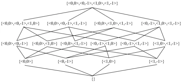
Solving a CSP can be seen as a search process over the lattice of the variable domains. For a given CSP (X,D,C) let us consider the complete domain lattice L defined by the elements obtained from the

power set of D partially ordered by set inclusion (⊆) and closed under arbitrary intersection (∩) and

union (∪). Figure 2.1 shows an example of a CSP P (with finite domains) and figure 2.2 the

corresponding domain lattice L.

Figure 2.1 An example of a CSP with finite domains. The figure represents the two axes x1 and x2, the four points are the domain set, the circumferences are the two constraints (inside c1 and outside c2). The solutions are the two points (<0,-1> and <1,-1>) inside the dashed area.

4 _{This extension will be later used, in subsection 4.2.1, for defining equivalent CSPs obtained by constraint decomposition,} which includes necessarily new variables.

P=(<x1,x2>,D1×D2,{c1,c2})

D1={0,1} D2={0,-1}

c1≡x12+ x22≤4 c2≡(x1-1)2+(x2-1)2≥4

c1

c2

16

Figure 2.2 Domain lattice of the previous example partially ordered by set inclusion (⊆).

The search procedure starts at the top of the domain lattice (the original domain D) and navigating over the lattice elements it will eventually stop, returning one of them. If it returns the bottom element

(the empty set {}) then the CSP has no solution.

In the example of figure 2.1 the returned element should be:

(i) {<0,-1>} or {<1,-1>} if the goal is to find at least one solution; (ii) {<0,-1>,<1,-1>} if the goal is to compute the space of all solutions;

(iii) {<0,-1>} if the goal is to find the solutions that minimize x12+ x22.

The navigation over the lattice elements usually alternates pruning with branching steps and ends

whenever a stopping criterion is satisfied.

2.1.1

Pruning

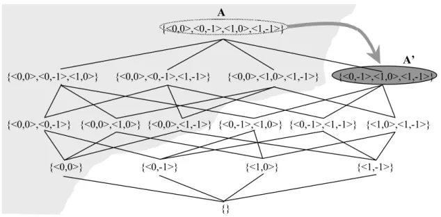
The pruning consists on jumping from an element of the lattice to a smaller element (with respect to

the set inclusion partial order) as a result of applying an appropriate filtering algorithm which eliminates some value combinations that are inconsistent with the constraints. All lattice elements

containing value combinations that were eliminated in the pruning step will not be considered any further. The elements remaining form a sub-lattice with non-eliminated value combinations as a top element.

Figure 2.3 shows the result of applying a pruning step on the top element of the domain lattice of the above example. The combination of values x1=0 and x2=0, proved to be inconsistent with the

constraints by some filtering algorithm, is absent in the resulting lattice.

{<0,0>,<0,-1>,<1,0>,<1,-1>}

{<0,0>,<0,-1>,<1,0>} {<0,0>,<0,-1>,<1,-1>} {<0,0>,<1,0>,<1,-1>} {<0,-1>,<1,0>,<1,-1>}

{<0,0>,<0,-1>} {<0,0>,<1,0>} {<0,0>,<1,-1>} {<0,-1>,<1,0>} {<0,-1>,<1,-1>} {<1,0>,<1,-1>}

{<0,0>} {<0,-1>} {<1,0>} {<1,-1>}