Todos os direitos reservados.
É proibida a reprodução parcial ou integral do conteúdo
deste documento por qualquer meio de distribuição, digital ou
impresso, sem a expressa autorização do
REAP ou de seu autor.
Joint Analysis of the Discount Factor and Payoff
Parameters in Dynamic Discrete Choice Games
Tatiana Komarova
Fabio A. Miessi Sanches
Daniel Silva Junior
Sorawoot Srisuma
Joint Analysis of the Discount Factor and Payo¤
Parameters in Dynamic Discrete Choice Games
Tatiana Komarova
Fabio A. Miessi Sanches
Daniel Silva Junior
Sorawoot Srisuma
Tatiana Komarova
Joint Analysis of the Discount Factor and Payo¤
Parameters in Dynamic Discrete Choice Games
y
Tatiana Komarova
London School of Economics
Fabio A. Miessi Sanches
University of São Paulo
Daniel Silva Junior
University of Coventry
Sorawoot Srisuma
University of Surrey
February 02, 2016
Abstract
Most empirical models of dynamic games assume the discount factor to be known and focus on the estimation of the payo¤ parameters. However, the discount factor can be identi…ed when
the payo¤s satisfy parametric or other nonparametric restrictions. We show when the payo¤s take the popular linear-in-parameter speci…cation, the joint identi…cation of the discount factor
and payo¤ parameters can be simpli…ed to a one-dimensional model that is easy to analyze. We also show that switching costs (e.g. entry costs) that often feature in empirical work can be identi…ed in closed-form, independently of the discount factor and other speci…cation of the
payo¤ function. Our identi…cation strategies are constructive. They lead to easy to compute estimands that are global solutions. Estimating the discount factor permits direct inference on
borrowing rate. Our estimates of the switching costs can be used for speci…cation testing. We illustrate with a Monte Carlo study and the dataset from Ryan (2012).
JEL Classification Numbers: C14, C25, C61
Keywords: Discount Factor, Dynamic Games, Identi…cation, Estimation, Switching Costs Earlier versions of this research were circulated under the title “Identifying Dynamic Games with Switching Costs”. We thank Kirill Evdokimov, Emmanuel Guerre, Koen Jochmans, Arthur Lewbel, Oliver Linton, Aureo de Paula, Martin Pesendorfer, Yuya Sasaki, Richard Spady, Pasquale Schiraldi and seminar participants at CREATES, GRIPS, Johns Hopkins University, LSE, NUS, Queen Mary University of London, Stony Brook University, University of Cambridge, University of São Paulo, and participants at Bristol Econometrics Study Group (2014), AMES (Taipei), EMES (Toulouse) and IAAE (London) for comments.
1
Introduction
A structural study involves modeling the economic problem of interest based on some primitives that govern an economic model. The primitives have a clear interpretation. The empirical goal is to estimate them, which can then be used for counterfactual analysis. Our paper studies some identi…cation and estimation aspects for a stationary dynamic discrete game that generalizes the single agent Markov decision problem surveyed in Rust (1994). The primitives of the games we consider consist of players’ (per-period) payo¤ functions, discount factor, and Markov transition law of the variables in the model.
There is anecdotal evidence from the literature on single agent models that implies that dynamic games are generally not identi…ed nonparametrically. For example, Manski (1993) shows that the discount factor cannot be identi…ed jointly with the payo¤ function that is nonparametric; Magnac and Thesmar (2002) show the payo¤ function cannot be identi…ed even if all other primitives of the model are known; Norets and Tang (2014) show the payo¤ function can only be partially identi…ed when the distributions of unobservable state variables are unknown with discrete observable states. But identi…cation is possible with more structure on the model. For examples, see Pesendorfer and Schmidt-Dengler (2008), Bajari, Chernozhukov, Hong and Nekipelov (2009), Blevins (2014), Chen (2014), as well as Fang and Wang (2014). Hence, in spite of the under-identi…ed nature of a general structural dynamic model, many fruitful empirical research can be, and has been, conducted based on these dynamic models using the theoretical results as guide.
Empirical applications of dynamic games often focus on the estimation of the parametric pay-o¤ functions and seemingly always assume the value of the discount factor to be known. An in-discriminating list of examples include: Beresteanu, Ellickson and Misra (2010), Collard-Wexler (2013), Dunne, Klimek, Roberts and Xu (2013), Gowrisankaran, Lucarelli, Schmidt-Dengler and Town (2010), Igami (2015), Lin (2012), Sanches, Silva and Srisuma (2014), Snider (2009) and Suzuki (2013). There appears to be no formal justi…cation as to why the discount factor has to be presumed known rather than estimated. Commonly cited reasons, if any is given at all, include precedence from the single agent literature, lack of identi…cation, numerical di¢culties (e.g. intractability or convergence failure) and post-estimation issues (e.g. implausible or imprecise estimates). The un-derlying sources for the …rst reasoning can also be traced to the other closely related, but distinct, issues.1,2
1Some noted estimation attempts in the single agent context include: Rust (1987, pp. 1023), who says “I was not
able to precisely estimate the discount factor”, while Slade (1998, pp. 102) also …xes the discount factor after “it was found that the objective function is fairly ‡at” over some range.
2Estimation of the discount factor in some related …nite-time horizon models is more standard, and with more
Identi…cation is a property of the model. It is customary to translate the behavioral condition that de…nes (parametric, point-) identi…cation into a loss function with a unique minimum for the purpose of estimation. There are often many candidates of loss functions. A positive identi…cation for one is su¢cient to identify the model. However, in general, verifying that a nonlinear function of several variables has a unique minimum point is a di¢cult mathematical task. The degree of di¢culty can depend crucially on the choice of the loss function. This also relates directly to the practical aspects of computing the estimand.3 Particularly it may not even be a trivial assumption to assume
that one can always …nd the global minimum of a nonlinear loss function with many parameters in a dynamic game due to intractable components of the model. Therefore, in practice, implausible estimates may also arise due to a purely a numerical reason even if the model is correctly speci…ed.4
Our paper aims to show that it is not necessary to assume the discount factor a priori in order to analyze empirical games. We consider two important special cases. First, we show that when payo¤s take a linear parameterization, joint identi…cation of the discount factor and payo¤ parameters can be analyzed as a one-parameter model irrespective of the number of payo¤ parameters. Second, for games with switching costs (such as entry costs and scrap values), we show the switching cost parameters can be identi…ed in closed-form independently of the discount factor and speci…cation of other parts of the payo¤ function. Our identi…cation strategies are constructive. The corresponding estimands are easy to compute. An important feature is they aim to obtain global solutions to potentially complex optimization problems in a transparent manner. Then the estimates of the discount factor permit testing of borrowing costs and other dynamic considerations directly. Also the closed-form estimators for the switching costs can be used for speci…cation testing. E.g. testing the mode of competition amongst …rms, by comparing them with estimates from existing methods that explicitly specify the entire payo¤ function.
The non-identi…cation argument in Manski (1993) does not preclude us from studying the identi-…cation of the discount factor since the payo¤ functions employed in practice satisfy a priori speci…ed parametric and/or other nonparametric restrictions. However, even in a single agent model with a known discount factor, establishing that the parametric payo¤ parameters are identi…ed is di¢cult due to the nonlinear nature of the model that contains an intractable value function. Furthermore in dynamic games there may be multiple equilibria, subsequently the model may beincomplete (Tamer (2003)). We proceed in the same way as Pesendorfer and Schmidt-Dengler (2008) and Bajari et
reported (e.g. see Hotz and Miller (1993)).
3For example, as Hotz, Miller, Sanders and Smith (1994) noted in their footnote 13 on pp. 280 that: “There is
nothing inherent in our method which precludes estimation of [the discount factor] ... our primary reason for not estimating was the intractability it presented for implementing the ML [a competing] estimator.”
4Since a structural model is interpreted as an approximation of the data generating process, misspeci…cation here
al. (2009) and study identi…cation using the implied expected discounted payo¤s that generates the data based on the observed transition probabilities. More speci…cally we take the model to be the collection of implied expected discounted payo¤s as a mapping from the parameter space. Such model reduces the degree of intractability of the model and circumvents the issue of incomplete-ness, and is the basis for all what is known as “two-step” estimation methods in the literature (e.g. Aguirregabiria and Mira (2007), Bajari, Benkard, Levin (2007), Pakes, Ostrovsky and Berry (2007), Pesendorfer and Schmidt-Dengler (2008)).
We …rst consider the linear-in-parameter payo¤ speci…cation due to its overwhelmingly com-mon usage in empirical work; examples include those in the list of applications above.5 When the
discount factor is known, the corresponding implied expected discounted payo¤ also takes the linear-in-parameter structure. Various computational exploits of this linear structure have been noted, e.g. see Miller, Sanders and Smith (1994), Bajari, Benkard, Levin (2007), Bajari et al. (2009), and Sanches, Silva and Srisuma (2015). In particular Sanches et al. (2015) translate the identi…cation condition for the linear payo¤ parameter in terms of the uniqueness of the minimum Euclidean norm between the observed and model implied expected discounted values. Their estimator has the famil-iar closed-form OLS expression and condition for identi…cation can be given in terms of the full rank condition of a matrix. See Assumption B1 in Sanches et al. (2015). It is worth emphasizing that their Assumption B1 is also necessary for consistent estimation of any two-step estimator in that setting.
When the discount factor is unknown and taken as part of the parameter space the model becomes intrinsically nonlinear. Existing conditions that ensure identi…cation in a nonlinear parametric model in econometrics can be hard to verify and the scope of applications is limited by stringent conditions; see Komunjer (2012) for recent results. Here we show that the identi…cation for games with linear-in-parameter payo¤s can be analyzed exhaustively even when the parameter space is large. We follow the approach in Sanches et al. (2015) and expand the parameter space to include the discount factor. The least squares framework enables us to simplify the problem by just considering a one-dimensional path of the parameter space. In particular, for any value of the discount factor, there exists a vector of payo¤ parameters that minimize the least squares that has a closed-form OLS expression. The pro…led distance becomes a mapping from [0;1] to R. Therefore an exhaustive analysis of identi…cation for the discount factor reduces to simply evaluating a function with one argument over a small domain. Once the identi…cation of the discount factor is established it can be taken as known. The payo¤ parameters is then identi…ed if an analogous condition to Assumption
5Other speci…cations that have been employed are often motivated by the need to impose additional constraints.
B1 in Sanches et al. (2015) holds.
When the parameterization of the payo¤ function is not linear we focus on reducing the parameter space instead of studying the joint identi…cation of the discount factor and payo¤ parameters. Our approach re‡ects a common practice that not all components of the payo¤ function need to be treated in the same way. Parts of the payo¤ function, such as variable pro…ts, can be estimated directly using economic theory if relevant data are available. These serve as exclusion restrictions (e.g. see Berry and Haile (2010, 2012)). The remaining components aredynamic parameters of the game that have to be estimated using the structure of the dynamic models. One of the most prevalent type of dynamic parameters arises from players choosing di¤erent actions from the previous period. Speci…c examples include entry cost and scrap value in games with entry, menu costs in pricing problems, as well as adjustment costs in investment decisions. We refer to these as switching costs. Switching costs, by de…nition, have built-in nonparametric structures that impose how they can appear in the payo¤ function.
We show that switching costs can be identi…ed, in a closed-form, independently of the discount factor and speci…cation of the remaining components of the payo¤ function. It may not come as a surprise that such result requires some restrictions on the payo¤s as well as the dependence structure of the controlled Markov process. However, the conditions we impose can be motivated empirically and have been frequently assumed in the empirical literature. Speci…cally, we assume that, whether a player may incur a switching cost in each period is only determined by her own action. The state variables, such as past actions of all players, can otherwise a¤ect today’s switching costs in an arbitrary way. We also require that the remaining components of the payo¤ function do not depend on past actions (this can be relaxed to allow dependence of a …nite time lag). The latter condition is satis…ed by typical payo¤ components. E.g. variable pro…ts that are determined by the competition between players depend only on those present in the game (for instance a Cournot or an auction game), as well as …xed operating costs. We also limit the feedback of past actions in the Markov process. We assume that the past actions do not a¤ect the transition law of future states conditional on today’s actions and states. Our conditional independence requirement is a testable assumption, and is weaker than the frequently assumed condition that state variables other than actions are strictly exogenous. Examples of empirical models that satisfy these assumptions can be found in the applications cited above amongst many others.
switching costs and some nuisance parameters that depend on all primitives of the game. In a single agent dynamic decision model, the switching costs can then be identi…ed by simply di¤erencing out the nuisance parameters. For a dynamic game, the nuisance terms can be eliminated by a projection that can be interpreted as a generalized di¤erence. Therefore the switching costs can be identi…ed up to some location normalizations that accounts for the nonparametric speci…cation of the remaining components of the payo¤ function. Our approach to eliminate the nuisance term therefore shares some similarities with the pair-wise di¤erencing approach that is useful for the estimation of com-plicated nonlinear models (e.g. see Honoré and Powell (2005)). Notably, the pair-wise di¤erence estimator that Hong and Shum (2010) propose for a single agent dynamic investment model can also be computed without the knowledge of the discount factor.6
The estimation of dyamic games is generally considered to be a numerically challenging task. Analogous to the identi…cation argument above, the choice of the estimation methodology can be crucial for practical analysis of dynamic games. Traditional approach in econometrics takes consistent estimation for granted and focuses on e¢ciency. However, even consistency of a sensible looking estimation procedure may be problematic in practice due to the complicated nature of dynamic games. E.g. see Appendix A in Srisuma (2013), and also a series of papers related to sequential estimation methods (Pesendorfer and Schmidt-Dengler (2010), Kasahara and Shimotsu (2012) and Egesdal, Lai and Su (2015)). In this paper we focus on the simplicity of implementation. We adopt the approach of Sanches et al. (2015). The contribution of that paper highlights the computational advantages that least squares criterions in expected payo¤s have over its dual representation in terms of the choice probabilities; particularly as proposed by Pesendorfer and Schmidt-Dengler (2008).7
Importantly they show the estimators are in fact asymptotically equivalent but the numerical e¤orts in computing the latter can be substantially higher.8 It can be shown that these advantages are
conserved when the parameter space expands to include the discount factor.
Our estimators can then be constructed according to our identi…cation arguments. Our pro…ling estimator uses the closed-form OLS expression for the linear payo¤ parameters in terms of the
6The motivation behind Hong and Shum (2010)’s estimator is actually to avoid the computation of the value
function rather than constructing a robust estimator. In particular they di¤erence out the future discounted payo¤s between two economic agents if their investment accumulations are (nearly) equal under a deterministic state transition rule.
7There are also other authors have also proposed estimators that minimize expected payo¤s. In particular, under
the linear-in-parameter assumption, the estimators of Miller, Sanders and Smith (1994) and Bajari et al. (2009) take and an IV form.
8The class of estimators proposed by Pesendorfer and Schmidt-Dengler (2008) has been well received. It includes
discount factor. Therefore our joint estimation of the discount factor and the payo¤ parameters can be conducted by a simple and exhaustive one-dimensional search over the support of the discount factor. In games with switching costs, closed-form estimation of switching costs serves to reduce the number of parameters to be estimated. The dimensionality reduction can be substantial in a game with large dimensions; as the number of unrestricted switching costs for each player grow at a quadratic rate with respect to the number of possible actions, which then grows exponentially fast with the number of players for every state.
We provide a Monte Carlo study to analyze some basic statistical properties of our proposed estimators. We then use the dataset from Ryan (2012) to estimate a dynamic game played between …rms in the US Portland cement industry. In our version of the game, …rms choose whether to enter the market as well as decide on the capacity level of operation (…ve di¤erent levels). We assume …rms compete in a capacity constrained Cournot game, so the period pro…t can be estimated directly from the data as done in Ryan. The remaining part of the payo¤ consists of …xed operating costs and 25 switching cost parameters. Other dynamic parameters we estimate include the discount factor and …xed operating cost. We estimate the model twice. Once using the data from before 1990, and once after 1990, which coincides with the date of the 1990 Clean Air Act Amendments (1990 CAAA). Our switching costs estimates generally appear sensible, having correct signs and relative magnitudes. They show that …rms entering the market with a higher capacity level incur larger costs, and suggest that increasing capacity level is generally costly while a reduction can return some revenue. We also …nd that operating and entry costs are generally higher after the 1990 CAAA, which supports Ryan’s key …nding. We are also able to estimate the discount factor with reasonable precision.
The remainder of the paper is organized as follows. Section 2 de…nes the theoretical model and states the modeling assumptions. Section 3 considers the joint identi…cation of discount factor and payo¤ parameters under the linear speci…cation. Section 4 shows the closed-form identi…cation of switching costs. Section 5 illustrates the use of our estimator with simulated and real data. Section 6 concludes.
2
Model and Assumptions
We consider a game withI players, indexed byi2 I =f1; : : : ; Ig, who compete over an in…nite time horizon. The variables of the game in each period are action and state variables. The action set of each player isA=f0;1; : : : ; Kg. Letat = (a1t; : : : ; aIt)2AI. We will also occasionally abuse the notation and writeat= (ait; a it)wherea it = (a1t; : : : ; ai 1t; ai+1t: : : ; aIt)2AI. Player i’s information set is represented by the state variables sit 2S, where sit = (xt; "it) such that xt 2 X, for some compact setX RdX. Statex
by the econometrician, while "it = ("it(0); : : : ; "it(K))2RK+1 is private information only observed by player i. We de…ne st (xt; "t) and "t ("1t; : : : ; "It). Future states are uncertain. Players’ actions and states today a¤ect future states. The evolution of the states is summarized by a Markov transition law P (st+1jst; at). Each player has a payo¤ function, ui : AI S ! R, which is time separable. Future period’s payo¤s are discounted at the rate 2[0;1).
The setup described above, and the following assumptions, which we shall assume throughout the paper, are standard in the modeling of dynamic discrete games. For examples, see Aguirregabiria and Mira (2007), Bajari, Benkard and Levin (2007), Pakes, Ostrovsky and Berry (2007), Pesendorfer and Schmidt-Dengler (2008).
Assumption M1 (Additive Separability): For all i; ai; a i; x; "i:
ui(ai; a i; x; "i) = i(ai; a i; x) +
X
a0
i2A
"i(a0i) 1[ai =a0i].
Assumption M2 (Conditional Independence I): The transition distribution of the states has the following factorization for all x0; w"0; x; "; a:
P(x0; "0jx; "; a) =Q("0)G(x0jx; a);
where Q is the cumulative distribution function of "t and G denotes the transition law of xt+1
conditioning on xt; at.
Assumption M3 (Independent Private Values): The private information is independently distributed across players, and each is absolutely continuous with respect to the Lebesgue measure
whose density is bounded on RK+1 with unbounded support.
Assumption M4 (Discrete Public Values): The support of xt is …nite so that X =
x1; : : : ; xJ for some J <1.
The game proceeds as follows. At time t, each player observes sit and then chooses ait simulta-neously. Action and state variables at time t a¤ectssit+1. Upon observing their new states, players
choose their actions again and so on. We consider a Markovian framework where players’ behavior is stationary across time and players are assumed to play pure strategies. More speci…cally, for some
conditional on xt for some pure Markov strategy pro…le( 1; : : : ; I). The decision problem for each player is to solve, for any si,
max
ai2f0;1gfE[ui(ait; a it; si)jsit = si; ait=ai] + E[Vi(sit+1)jsit=si; ait=ai]g; (1)
whereVi(si) =
1
X
=0
E[ui(ait+ ; a it+ ; sit+ )jsit=si]:
The expectation operators in the display above integrate out variables with respect to the probability distribution induced by the equilibrium beliefs and Markov transition law. Vi denotes the value function. Note that the beliefs and primitives completely determine the transition law for future states. Any strategy pro…le that solves the decision problems for alliand is consistent with the beliefs satis…es is an equilibrium strategy. Pure strategies Markov perfect equilibria have been shown to exist for such games (see Aguirregabiria and Mira (2007), Pesendorfer and Schmidt-Dengler (2008)). We consider identi…cation based on the joint distribution of the observables, namely(at; xt; xt+1),
which is consistent with a single equilibrium play. The ideal data set is therefore a long time series from a single market. Although more commonly, datasets used in empirical work have short panel from multiple markets, the joint distribution of the observables can still be identi…ed if they are generated from the same equilibrium.9 The primitives of the game under this setting consists of (f igIi=1; ; Q; G). Throughout the paper we shall also assume G and Q to be known (the former can be identi…ed from the data).
3
Identi…cation with Linear-in-Parameter Payo¤s
In this section we consider games where payo¤s have a linear-in-parameter speci…cation. Section 3.1 de…nes identi…cation for the parameter of interest and provide some representation lemmas based on the linear payo¤ structure. Section 3.2 studies identi…cation by pro…ling.
3.1
De…nition of Identi…cation and Some Representation Lemmas
We assume the following assumption holds throughout this section.
Assumption M5 (Linear-in-Parameter): For all i; ai; a i; x:
i(ai; a i; x; ) = i0(ai; a i; x) + > i1(ai; a i; x),
where i0 is a known real value function, i1 is a known p dimensional vector value function and
belongs to Rp.
The role of i0 is to represent the payo¤ components that are identi…able without the knowledge
of the discount factor. In practice i0 and possibly parts of i1 may have to be estimated (e.g. see
Section 5.2). For the purpose of identi…cation they can be treated as known.
The primitives of interest belong to B , where B= [0;1) and =Rp for some non-negative integer p. We are interested in the data generating discount factor and payo¤ parameters, which we denote by 0 and 0 respectively. We …rst de…ne the choice speci…c expected payo¤s for choosing
action ai prior to adding the period unobserved state variable, which is computed for di¤erent and , for any i; ai and x:
vi(ai; x; ; ) =E[ i(ai; a it; xt; )jxt =x] + gi(ai; x; ; ); (2)
wheregi(ai; x; ; ) E[Vi(sit+1; ; )jait =ai; xt=x]withVi(si; ; ) P1=0 E[ui(at+ ; sit+ ; )jsit =s and ui(at; sit; ) i(at; xt; )+
P
a0
i2A"it(a 0
i) 1[ait =a0i]. Note that the expectations here are taken with respect to the observed choice and transition probabilities that are consistent with 0 and 0.
We consider the relative payo¤s in (2) with action 0as the base, so that for all i; ai >0and x:
vi(ai; x; ; ) = E[ i(ai; a it; x; )jxt=x] + gi(ai; x; ; ); (3)
where vi(ai; x; ; ) vi(ai; x; ; ) vi(0; x; ; ); i(ai; a i; x; ) i(ai; a i; x; ) i(0; a i; x; ) for all ai, and gi(ai; x; ; ) gi(ai; x; ; ) gi(0; x; ; ). Using Hotz-Miller’s inversion, it follows that vi(ai; x; 0; 0) is identi…ed from the data for all i; ai; x. We take each pair ( ; ) to be a structure of the (empirical) model and its implied expected payo¤s, denoted by V ;
f vi(ai; x; ; )gi;ai;x2I A X, to be its corresponding reduced form.
10,11 We can then de…ne
identi…-cation using the notion of observational equivalence in terms of the expected payo¤s.
Definition I1 (Observational Equivalence): Any distinct ( ; )and ( 0; 0) in B are observationally equivalent if and only if V ; =V 0; 0.
Definition I2 (Identification): An element in B , say ( ; ), is identi…ed if and only if ( 0; 0) and ( ; ) are not observationally equivalent for all ( 0; 0)6= ( ; ) in B .
The following lemma relates the parameters we want to identify to what can be observed.
10The empirical model is a pseudo-model. Because we do not use the equilibrium probabilities of the dynamic game
corresponding to ; . We only consider the implied expected payo¤s computed using the equilibrium beliefs that generate the data.
11It is equivalent to de…ne the reduced forms in terms of expected payo¤s is equivalent to de…ning them in terms of
Lemma 1: Under M1 - M5, we have for all i; ai >0, vi(ai; x; ; )can collected in the following
vector form for all ( ; )2 B :
vai
i ( ; ) = R
ai
i0 + H
ai
i (IJ L) 1Ri0 (4)
+ Rai
i1+ H
ai
i (IJ L) 1Ri1
+ Hai
i (IJ L) 1 i;
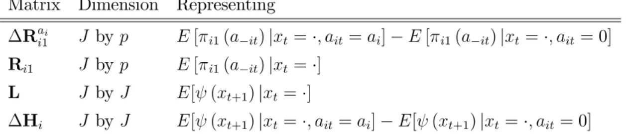
where the elements in the equation above are collected and explained in Tables 1 and 2.
Matrix Dimension Representing
Rai
i1 J by p E[ i1(a it)jxt= ; ait =ai] E[ i1(a it)jxt= ; ait= 0]
Ri1 J by p E[ i1(a it)jxt= ]
L J by J E[ (xt+1)jxt= ]
Hi J by J E[ (xt+1)jxt= ; ait =ai] E[ (xt+1)jxt = ; ait= 0]
Table A. The matrices consist of (di¤erences in) expected payo¤s and probabilities. The latter represent conditional expectations for any function of xt+1.
Vector Representing
i EhPa0
i2A"it(a 0
i) 1[ait =a0i] xt=
i
Rai
i0 E[ i0(ait; a it; xt)jxt= ; ait =ai] E[ i0(ait; a it; xt)jxt= ; ait= 0]
Ri0 E[ i0(at; xt)jxt= ]
(IJ L) 1R ij
P1
=0 E[ ij(at+ ; xt+ )jxt= ]
Hai
i (IJ L) 1R ij
P1
=1 E[ ij(at+ ; xt+ )jxt= ; ait =ai]
P1
=1 E[ ij(at+ ; xt+ )jxt = ; ait = 0]
Hai
i (IJ L) 1 i
P1
=1 E
hP
a0
i2A"it+ (a 0
i) 1[ait+ =ai0] xt= ; ait =ai
i
P1
=1 E
hP
a0
i2A"it+ (a 0
i) 1[ait+ =a0i] xt = ; ait = 0
i
Table B. The J by 1vectors represent (di¤erences in) expected payo¤s.
Proof: This is a slight variation of Lemma R in Sanches et al. (2014).
Lemma 1 is simply a vectorization (across states) of the di¤erences in discounted expected payo¤s for player i from choosing action ai relative to action0. From the data we can identify vaii( 0; 0)
for all i; ai > 0. Hence, to identify ( 0; 0), it is enough to show that for all ( ; ) 6= ( 0; 0),
vai
i ( ; )6= v ai
i ( 0; 0) for someiand ai. Our next lemma provides a characterization as to how
Lemma 2: Under M1 - M5, for any i; ai >0 and ( ; );( 0; 0)2 B :
vai ( ; ) via( ; 0) = Rai
i1 + H
ai
i (IJ L) 1Ri1 ( 0); (5)
vai ( 0; 0) via( ; 0) = ( 0) Hai
i (IJ 0L)
1
(IJ L) 1(Ri0+Ri1 0+ i): (6)
And ( ; ) is identi…able if and only if there is no other ( 0; 0) such that for all i; ai >0:
vai ( 0; 0) vai ( ; 0) = vai ( ; ) vai ( ; 0):
Proof: Follows from some algebra based on equation (4).
Lemma 2 illustrates the nature of the identi…cation problem we have at hand. We highlight the following particulars:
(i)If the discount rate is assumed to be known, from (5), a su¢cient condition for vai ( 0; )6=
va
i ( 0; 0) when 6= 0 is that R
ai
i1 + H
ai
i (IJ L) 1Ri1 has full column rank for some i; ai >0.
(ii)If the payo¤ function is assumed to be known, from (6), a su¢cient condition for va i (
0; 0)6=
vai ( ; 0) when =6 0 is that (Ri0+Ri1 0+ i)6= 0 and Hiai is invertible some i; ai >0.
(iii) Supposepis large relative toJ. Then for anyi; ai >0such that Rai1i+ H
ai
i (IJ L) 1Ri1
has rank J, and for any 0; 6= 0 that via( 0; 0) 6= vai ( ; 0), by equating (5) and (6), we can
always …nd such that va
i (
0; 0) = va i ( ; ).
Point (i) shows that su¢cient conditions for identi…cation of the payo¤ parameters when the discount rate is assumed known can be easily stated and veri…ed. More generally the su¢cient condition for the identi…cation of the payo¤ parameter can be stated in terms of the full column rank of the matrix that stacks together Rai
i1 + H
ai
i (IJ L) 1Ri1 over alli and ai. In the case we
can identify the payo¤ function directly from the data, (ii) shows that the discount factor can also be identi…ed and provide one type of su¢cient conditions that can be readily checked. Point (iii) shares the intuition along the line of Manski (1993) that when the parameterization on the payo¤ function is too rich, ( ; ) may not identi…able in B .
From Lemma 2, it is also apparent that we should be able to identify ( 0; 0) jointly when the
change in the vector of expected payo¤s from altering the discount factor moves in a di¤erent direction to the change caused by altering the payo¤ parameters.
3.2
Pro…ling
Pro…ling makes use of the fact that for each the expected payo¤s are linear in . We de…ne
mai
i ( ; ) v
ai
i ( 0; 0) vaii( ; ), so that we can write:
mai
i ( ; ) =a ai
i ( ) B
ai
where from (4),
aai
i ( ) = v
ai
i ( 0; 0) Rai0i H
ai
i (IJ L) 1(Ri0+ i);
Bai
i ( ) = R
ai
i1 + H
ai
i (IJ L) 1Ri1:
It is clear that for any given , mai
i ( ; ) is linear in . The system of equations above can be
expanded by stacking them across all i and ai. In doing so we obtain the following vector value
function, m:B !RIJ K :
m( ; ) = a( ) B( ) ;
where a( )is a IJK by 1 vector and B( ) is a IJK by p matrix. Let M( ; ) km( ; )k, i.e. the Euclidean norm of m( ; ). Then by construction,
M( ; ) = 0 if ( ; ) = ( 0; 0);
and any other ( ; )such that M( ; ) = 0 is observationally equivalent to ( 0; 0) by the property
of the norm. Next we pro…le out . Let y denotes the Moore-Penrose generalized inverse of a matrix.
For each , we de…ne:
( ) = B( )>B( ) yB( )>a( );
so that ( )is a least squares solution to min 2 M( ; ). Then we de…ne:
M ( ) =M( ; ( )):
By construction it also holds that
M ( ) = 0 if = 0:
In this way we can temporarily reduce the parameter space in the identi…cation problem to a one-dimensional one. The reasoning is analogous to pro…ling in an estimation routine. Particularly we can ignore any that does not lie in arg min 2 M( ; )since necessarily,
M( ; )>M( ; ( )) 0:
Therefore ( 0; 0) is identi…ed when M ( ) has a unique minimum and min 2 M( 0; ) has a
unique solution.
Theorem 1: ( 0; 0) is identi…able if
M ( ) = 0 if and only if = 0;
Proof: Suppose ( 0; 0) is identi…able. If there is 0 6= 0 such that M ( 0) = 0, then
vai
i ( 0; 0) = vaii(
0;
( 0)) for all i; ai by the property of the norm. Since is closed, by the projection theorem, ( 0) exists and is the unique element in . This leads to a contradiction since ( 0; 0) and ( 0; ( 0)) are observationally equivalent. Next, suppose that B( 0) does not
have full column rank. Let 0 be another element in arg min 2 M( 0; )that di¤ers from 0. Since M( 0; ) 0 for all 2 and M( 0; 0) = 0, M( 0; 0) = 0. Thus ( 0; 0) and ( 0; 0) are
observationally equivalent, also a contradiction.
Comments on Theorem 1:
(i) High Level Assumptions. Conditions in Theorem 1 are high level as we do not relate them to
the underlying primitives of the model. However, they are statements made on objects that observed or can be consistently estimated nonparametrically (as other conditions used in all of our theorems in this paper).
(ii) Feasible Check and Estimation. Since we have reduced the identi…cation problem to a single-parameter that can reside only in a narrow range, there is no need to refer to complicated results for the identi…cation of a general nonlinear model. Since it is possible to estimate M ( ) consistently for all , one can simply plot the sample counterpart of M over Bfor an exhaustive analysis of the
problem. Once the minimum of M is found, the corresponding rank matrix can then be checked.
This is indeed one way to estimate the discount factor, namely by grid search. We can detect an identi…cation problem if the sample counterpart of M contains a ‡at region at the minimum, or when the sample counterpart of B( 0) does not have full column rank.
4
Identi…cation of the Switching Costs
In this section we consider games with switching costs. Section 4.1 introduces the speci…c structures of the payo¤ function and an additional conditional independence assumption. Section 4.2 derives the closed-form expressions for the switching costs. Throughout this section we do not need M5, but will continue to assume that M1 - M4 hold.
4.1
Games with Switching Costs
Assumptions M1 - M4 are now be updated accordingly by replacingxwith(x; w)everywhere. In addition we need the following assumptions.
Assumption N1 (Decomposition of Profits): For all i; ai; a i; x; w:
i(ai; a i; x; w) = i(ai; a i; x) + i(ai; x; w; i) i(ai; x; w);
for some known function i : A X AI ! f0;1g such that for any ai, i(ai; x; w; i) = 0 for all
x when w2W0
i(ai; x), where W
d
i(ai; x) w2A
I :
i(ai; x; w) = d for d= 0;1.
Assumption N2 (Conditional Independence II): The distribution of xt+1 conditional on at and xt is independent of wt.
The components of the decomposition of ican be interpreted as follows. idenotes the switching cost. i is an indicator function, modeled by the researcher, which takes value 1 if and only if
a switching cost is present. We de…ne i to be zero whenever i takes value zero. In a model
that contains switching costs, it must be the case that for some ai, W0
i(ai; ) will be non-empty
since it contains w 2 AI such that the action of player’s i coincides with ai. Hence it is possible to consider distinguishing i from i. Then i is to be interpreted as the residual of the payo¤s that excludes the switching costs. Assumption N1 also imposes some distinct exclusion restrictions. Firstly, switching costs of each player are not a¤ected by other players’ actions in the same period. However, players’ past actions and other state variables can have direct e¤ects on switching costs. Secondly, past actions are excluded from i. Typical components in i that are often modeled to satisfy the required exclusion restrictions include payo¤ derived from interactions between players at the stage game, as well as other …xed costs such as …xed operating costs. Furthermore, this does not mean that variables from the past cannot a¤ect i sincext can contain lagged actions and other state variables. N1 is assumed in many applications in the literature.
N2 imposes that knowing actions from the past does not help predict future state variables when the present action and other observable state variables are known. Note that N2 is not implied by M2. Therefore when xtcontains lagged actions N2 can be weakened to allow for dependence of other state variables with past actions. In many applications fxtg is assumed to be a strictly exogenous …rst order Markov process. Speci…cally this implies xt+1 is independent of at conditional on xt in addition to N2. In any case, unlike M2, N2 is a restriction made on the observables so it can be tested directly from the data.
Example 1 (Entry Cost): SupposeK = 1, then the switching cost at time t is
i(ait; xt; wt; i) i(ait; xt; wt) =ECi(xt; a it 1) ait(1 ait 1):
So for all x, W1
i(1; x) = w= (0; a i) :a i 2A
I 1 and W0
i(1; x) = w= (1; a i) :a i 2A
I 1 ,
and Wd
i(0; x) =
?.
Example 2 (Scrap Value): Suppose K = 1, then the switching cost at time t is
i(ait; xt; wt; i) i(ait; xt; wt) = SVi(xt; a it 1) (1 ait)ait 1:
So for allx,Wd
i(1; x) =
?and,W1
i(0; x) = w= (1; a i) :a i 2A
I 1 andW0
i(0; x) = w= (0; a i) :a i 2
Example 3 (General Switching Costs): Suppose K 1, then the switching cost at time
t is
i(ait; xt; wt; i) i(ait; xt; wt) =
X
a0
i;a00i2A
SCi(a0i; a
00
i; xt; a it 1) 1[ait =a0i; ait 1 =a00i; a
0
i 6=a
00
i]:
Here SCi(a0i; a00i; xt; a it 1) denotes a cost player i incurs from switching from action ait 1 = a00i to
ait =a0i, at the state (xt; a it 1). So for all x and a i, using just the de…nition of a switching cost
we can set SCi(a0i; a0i; x; a i) = 0 for all a0i. Therefore without any further restrictions: W1i(ai; x) = w= (a0
i; a i) :a0i 2An faig; a i 2AI 1 and W0
i(ai; x) = w= (ai; a i) :a i 2A
I 1 for all x.
Note that Examples 1 and 2 are just special cases of Example 3 when K = 1, with an additional normalization of zero scrap value and entry cost respectively.
Before giving the formal results we brie‡y provide an intuition as to why N1 and N2 are helpful for identifying the switching costs.
Exclusion and Independence
The essence of our identi…cation strategy is most transparent in a single agent decision problem
under a two-period framework. For the moment suppose I = 1. Omitting the i subscript, the
expected payo¤ for choosing action a >0 under M1 to M4 is, cf. (8),
v(a; x; w) = (a; x; w) + E[ (at+1; xt+1; wt+1)jat=a; xt=x; wt =w]:
N1 imposes separability and exclusion restrictions of the following type:
(a; x; w) = (a; x) + (a; x; w; ) (a; x; w);
where is a known indicator such that (a; x; w; ) = 0 whenever a 6= w. Therefore the
The direct e¤ect of past action is also excluded from the future expected payo¤ under N2, as
E[ (at+1; xt+1; wt+1)jat; xt; wt] simpli…es to E[ (at+1; xt+1; wt+1)jat; xt]. Therefore we can write
v(a; x; w) = (a; x) + (a; x; w; ) (a; x; w);
where (a; x) is a nuisance function that equals to (a; x) + E[ (at+1; xt+1; wt+1)jat=a; xt=x]. Any variation in v(a; x; w)induced by changes in w while holding(a; x) …xed can be traced only to changes in (a; x; w). Since is a free parameter, the switching costs can then be identi…ed up to a location normalization by di¤erencing over the support of w; e.g. through(v(a; x; w) v(0; x; w)) (v(a; x; w0) v(0; x; w0))for some reference pointw0.
This simple argument can be generalized to identify switching costs in dynamic games. However, the way to di¤erence out the nuisance function necessarily becomes more complicated. Particularly the nuisance function will then also vary for di¤erent past action pro…le since we have to integrate out other players’ actions using the equilibrium beliefs that depends on past actions. Relatedly there are also larger degree of freedoms to be dealt with as the nuisance function contains more arguments. The precise form of di¤erencing required can be formalized by a projection that enables the identi…cation of the switching costs up to some normalizations.12
4.2
Closed-Form Identi…cation
We begin by introducing some additional notations and representation lemmas. For any x; w, we denote the ex-ante expected payo¤s by mi(x; w) =E[Vi(xt; wt; "it)jxt=x; wt =w], where Vi is the value function de…ned in (1) that can also be de…ned recursively through
mi(x; w) = E[ i(at; xt; wt)jxt =x; wt=w] +E[
X
a0
i2A
"it(a0i) 1[ait=a0i]jxt=x; wt =w] (7)
+ E[mi(xt+1; wt+1)jxt=x; wt=w];
12Mathematically, for …xed a; x, our identi…cation problem under N1 and N2 in a single agent case is equivalent to identifying g2 that satis…es the relation:
g1(w) =c+g2(w);
for a known functiong1and anunknown constantc. In the case of a game, the relation generalizes to
g1(w) =
Z
c(x)h(dxjw) +g2(w);
and the choice speci…c expected payo¤s for choosing action ai prior to adding the period unobserved state variable is
vi(ai; x; w) = E[ i(ait; a it; xt; wt)jait=ai; xt=x; wt =w] (8)
+ E[mi(xt+1; wt+1)jait =ai; xt =x; wt=w]:
Bothmiandviare familiar quantities in this literature. Under Assumption N2,E[mi(xt+1; wt+1)jait; xt; wt] can be simpli…ed further to E[mei(ait; a it; xt)jait; xt; wt], where for all i; ai; a i; x, using the law of iterated expectation, mei(ai; a i; x) E[mi(xt+1; ait; a it)jait=ai; a it =a i; xt =x]. Then, for
ai > 0, let vi(ai; x; w) vi(ai; x; w) vi(0; x; w); i(ai; a i; x) i(ai; a i; x) i(0; a i; x), and mei(ai; a i; x) mei(ai; a i; x) mei(0; a i; x) for all i; a i; x. Furthermore, since the action space is …nite, the conditions imposed on i i by N1 ensures for each ai >0 we can always write the di¤erences of switching costs as
i(ai; x; w; i) i(ai; x; w) i(0; x; w; i) i(0; x; w) =
X
w02W
i(ai;x)
i; i(ai; x; w0) 1[w=w0]; (9)
where i; i(ai; x; w) i(ai; x; w; i) i(0; x; w; i)is only de…ned on the setW i (ai; x) W 1
i(ai; x)[ W1
i(0; x). To illustrate, we brie‡y return to Examples 1 - 3.
Example 1 (Entry Cost, Cont.): Here the only ai >0 is ai = 1. Since W1i(0; x) is empty
W
i (1; x) = W 1
i(1; x), and for any w= (0; a i), i; i(1; x; w) = ECi(x; a i) for all i; a i; x.
Example 2 (Scrap Value, Cont.): Similarly to the above, W
i (1; x) = W 1
i(0; x), and for
any w= (1; a i), i; i(1; x; w) = SVi(x; a i)for all i; a i; x.
Example 3 (General Switching Costs, Cont.): For any ai > 0, based on the de…nition of a switching cost alone, both W1
i(ai; x) and W 1
i(0; x) can be non-empty. So for all i; a i; x such
that a0i 6=ai:
i; i(ai; x; w) = SCi(ai;0; x; a i) when w= (0; a i), (10)
i; i(ai; x; w) = SCi(0; ai; x; a i) when w= (ai; a i),
i; i(ai; x; w) = SCi(ai; a 0
i; x; a i) SCi(0; a0i; x; a i) when w= (a0i; a i) for a0i 6=ai or0:
Note thatSCi(a0i; a00i; x; a i)can be recovered for anyai 6=a0i by taking some linear combination from
i; i(ai; x; a 0
i; a i) a
i;a0i2A A
.
Lemma 3: Under M1 - M4 and N1 - N2, we have for all i; ai >0 and a i; x; w:
vi(ai; x; w) =E[ i(ai; a it; xt)jxt=x; wt =w] +
X
w02W
i(ai;x)
i; i(ai; x; w
0) 1[w=w0]; (11)
where
i(ai; a i; x) i(ai; a i; x) + mei(ai; a i; x): (12)
Proof: Using the law of iterated expectation, under M3E[Vi(sit+1)jait =ai; xt; wt] =E[mi(xt+1; wt+1)ja
which simpli…es further, after another application of the law of iterated expectation and N2, to
E[mei(ai; a it; xt)jxt; wt]. The remainder of the proof then follows from the de…nitions of the terms de…ned in the text.
Lemma 3 says that the (di¤erenced) choice speci…c expected payo¤s can be decomposed into a sum of the …xed pro…ts at time tand a conditional expectation of a nuisance function of i consisting of composite terms of the primitives. In particular the conditional law for the expectation in (11), which is that of a it given (xt; wt), is identi…able from the data. Since a conditional expectation operator is a linear operator, and the support of wt is a …nite set with (K + 1)I elements, we can then represent (11) by a matrix equation.
Lemma 4: Under M1 - M4 and N1 - N2, we have for all i; ai >0and x:
vi(ai; x) =Zi(x) i(ai; x) +Qi(ai; x) i; i(ai; x); (13)
where vi(ai; x) denotes a (K+ 1) I
dimensional vector of normalized expected discounted pay-o¤s, f vi(ai; x; w)gw2AI, Zi(xt) is a (K+ 1)I by (K+ 1)I 1 matrix of conditional probabilities,
fPr [a it =a ijxt=x; wt=w]g(a i;w)2AI 1 AI, i(ai; x)denotes a(K+ 1)I 1 by1vector of f i(ai; a i; x)ga
Qi(ai; x) is a (K+ 1) I
by W
i (ai; x) matrix of ones and zeros, and i; i(ai; x) is a W 1
i(ai; x)
by 1 vector of i; i(ai; x; w) w2W
i(ai;x)
.
Proof: Immediate.
Let (Z)denote the rank of matrix Z, and MZ denotes a projection matrix whose null space is the column space of Z. We now state our …rst result.
Theorem 2: Under M1 - M4 and N1 - N2, for each i; ai > 0 and x, if (i) Qi(ai; x) has full column rank; (ii) (Zi(x)) + (Qi(ai; x)) = ([Zi(x) :Qi(ai; x)]), then Qi(ai; x)>MZi(x)Qi(ai; x) is non-singular, and
Proof: The full column rank condition of Qi(ai; x) is a trivial assumption. The no perfect collinearity condition makes sure there is no redundancy in the modeling of the switching costs. The rank condition (ii) then ensures MZi(x)Qi(ai; x) preserves the rank of Qi(ai; x). Therefore
Qi(ai; x)>MZi(x)Qi(ai; x)must be non-singular. Otherwise the columns ofMZi(x)Qi(ai)is linearly
dependent, and some linear combination of the columns in Qi(ai) must lie in the column space of
Zi(x), thus violating the assumed rank condition. The proof is then completed by projecting the
vectors on both sides of equation (13) by MZi(x)and solve for i; i(ai; x).
In order for condition (ii) in Theorem 2 to hold, it is necessary for researchers to impose some a priori structures on the switching costs. Before commenting further, it will be informa-tive to revisit Examples 1 - 3. For notational simplicity we shall assume I = 2, so that wt 2
f(0;0);(0;1);(1;0);(1;1)g. And since A = f0;1g in Examples 1 and 2, we shall also drop ai from
vi(ai; x) =f vi(ai; x; w)gw2AI and i(ai; x) =f i(ai; a i; x)ga i2AI 1.
Example 1 (Entry Cost, Cont.): Equation (13) can be written as
2 6 6 6 6 4
vi(x;(0;0))
vi(x;(0;1))
vi(x;(1;0))
vi(x;(1;1))
3 7 7 7 7 5 = 2 6 6 6 6 4
P i(0jx;(0;0))
P i(0jx;(0;1))
P i(0jx;(1;0))
P i(0jx;(1;1))
P i(1jx;(0;0))
P i(1jx;(0;1))
P i(1jx;(1;0))
P i(1jx;(1;1))
3 7 7 7 7 5 "
i(0; x)
i(1; x)
# + 2 6 6 6 6 4 1 0 0 0 0 1 0 0 3 7 7 7 7 5 "
ECi(x;0)
ECi(x;1)
#
;
where P i(a ijx; w) Pr [a it =a ijxt=x; wt=w]. A simple su¢cient condition that ensures condition (ii) in Theorem 3 to hold is when the lower half of Zi(x) has full rank, i.e. when
Example 2 (Scrap Value, Cont.): Equation (13) can be written as 2 6 6 6 6 4
vi(x;(0;0))
vi(x;(0;1))
vi(x;(1;0))
vi(x;(1;1))
3 7 7 7 7 5 = 2 6 6 6 6 4
P i(0jx;(0;0))
P i(0jx;(0;1))
P i(0jx;(1;0))
P i(0jx;(1;1))
P i(1jx;(0;0))
P i(1jx;(0;1))
P i(1jx;(1;0))
P i(1jx;(1;1))
3 7 7 7 7 5 "
i(0; x)
i(1; x)
# + 2 6 6 6 6 4 0 0 1 0 0 0 0 1 3 7 7 7 7 5 "
SVi(x;0)
SVi(x;1)
#
:
An analogous su¢cient condition that ensures condition (ii) in Theorem 3 to hold in this case is
P i(0jx;(0;0))=6 P i(0jx;(0;1)).
Example 3 (General Switching Costs, Cont.): SupposeK = 2, we consider vi(2; x) =
f vi(2; x; w)gw2AI,
2 6 6 6 6 6 6 6 6 6 6 6 6 6 6 6 6 6 4
vi(2; x;(0;0))
vi(2; x;(0;1))
vi(2; x;(0;2))
vi(2; x;(1;0))
vi(2; x;(1;1))
vi(2; x;(1;2))
vi(2; x;(2;0))
vi(2; x;(2;1))
vi(2; x;(2;2))
3 7 7 7 7 7 7 7 7 7 7 7 7 7 7 7 7 7 5 = 2 6 6 6 6 6 6 6 6 6 6 6 6 6 6 6 6 6 4
P i(0jx;(0;0)) P i(1jx;(0;0)) P i(2jx;(0;0))
P i(0jx;(0;1)) P i(1jx;(0;1)) P i(2jx;(0;1))
P i(0jx;(0;2)) P i(1jx;(0;2)) P i(2jx;(0;2))
P i(0jx;(1;0)) P i(1jx;(1;0)) P i(2jx;(1;0))
P i(0jx;(1;1)) P i(1jx;(1;1)) P i(2jx;(1;1))
P i(0jx;(1;2)) P i(1jx;(1;2)) P i(2jx;(1;2))
P i(0jx;(2;0)) P i(1jx;(2;0)) P i(2jx;(2;0))
P i(0jx;(2;1)) P i(1jx;(2;1)) P i(2jx;(2;1))
P i(0jx;(2;2)) P i(1jx;(2;2)) P i(2jx;(2;2))
3 7 7 7 7 7 7 7 7 7 7 7 7 7 7 7 7 7 5 2 6 6 4
i(2;0; x)
i(2;1; x)
i(2;2; x)
3 7 7 5(15) + 2 6 6 6 6 6 6 6 6 6 6 6 6 6 6 6 6 6 4
1 0 0 0 0 0 0 0 0 0 1 0 0 0 0 0 0 0 0 0 1 0 0 0 0 0 0 0 0 0 1 0 0 0 0 0 0 0 0 0 1 0 0 0 0 0 0 0 0 0 1 0 0 0 0 0 0 0 0 0 1 0 0 0 0 0 0 0 0 0 1 0 0 0 0 0 0 0 0 0 1
3 7 7 7 7 7 7 7 7 7 7 7 7 7 7 7 7 7 5 2 6 6 6 6 6 6 6 6 6 6 6 6 6 6 6 6 6 4
SCi(2;0; x;0)
SCi(2;0; x;1)
SCi(2;0; x;2)
SCi(2;1; x;0) SCi(0;1; x;0)
SCi(2;1; x;1) SCi(0;1; x;1)
SCi(2;1; x;2) SCi(0;1; x;2)
SCi(0;2; x;0)
SCi(0;2; x;1)
SCi(0;2; x;2)
3 7 7 7 7 7 7 7 7 7 7 7 7 7 7 7 7 7 5 :
we have 9 equations. Therefore we need at least three restrictions. For example by normalizing one type of switching costs to be zero. More speci…cally suppose SCi(0; ai; x; a i) = 0 for all ai > 0, then Qi(2; x) i; i(2; x) becomes
2 6 6 6 6 6 6 6 6 6 6 6 6 6 6 6 6 6 4
1 0 0 0 0 0 0 1 0 0 0 0 0 0 1 0 0 0 0 0 0 1 0 0 0 0 0 0 1 0 0 0 0 0 0 1 0 0 0 0 0 0 0 0 0 0 0 0 0 0 0 0 0 0
3 7 7 7 7 7 7 7 7 7 7 7 7 7 7 7 7 7 5 2 6 6 6 6 6 6 6 6 6 6 4
SCi(2;0; x;0)
SCi(2;0; x;1)
SCi(2;0; x;2)
SCi(2;1; x;0) SCi(0;1; x;0)
SCi(2;1; x;1) SCi(0;1; x;1)
SCi(2;1; x;2) SCi(0;1; x;2)
3 7 7 7 7 7 7 7 7 7 7 5 ;
and similar to the two previous examples, a su¢cient condition for condition (ii) in Theorem 2 to hold can be given in the form that ensures the lower third of Zi(x) to have full rank, which
is equivalent to the determinant of
0 B B @
P i(0jx;(2;0)) P i(1jx;(2;0)) P i(2jx;(2;0))
P i(0jx;(2;1)) P i(1jx;(2;1)) P i(2jx;(2;1))
P i(0jx;(2;2)) P i(1jx;(2;2)) P i(2jx;(2;2))
1 C C
A is
non-zero. Such normalization is an example of an exclusion restriction. A preferred scenario would be to use economic or other prior knowledge to assign values so known switching costs can be removed from the right hand side (RHS) of equation (15). Other restrictions, such as equality of switch costs so that the costs from switching to and from actions that may be reasonable in capacity or pricing games can be used instead of a direct normalization. For instance suppose that
SCi(ai; a0i; x; a i) = SCi(a0i; ai; x; a i) whenever ai 6=a0i, then Qi(2; x) i; i(2; x)becomes
2 6 6 6 6 6 6 6 6 6 6 6 6 6 6 6 6 6 4
1 0 0 0 0 0
0 1 0 0 0 0
0 0 1 0 0 0
0 0 0 1 0 0
0 0 0 0 1 0
0 0 0 0 0 1
1 0 0 0 0 0
0 1 0 0 0 0
0 0 1 0 0 0
3 7 7 7 7 7 7 7 7 7 7 7 7 7 7 7 7 7 5 2 6 6 6 6 6 6 6 6 6 6 4
SCi(2;0; x;0)
SCi(2;0; x;1)
SCi(2;0; x;2)
SCi(2;1; x;0) SCi(0;1; x;0)
SCi(2;1; x;1) SCi(0;1; x;1)
SCi(2;1; x;2) SCi(0;1; x;2)
3 7 7 7 7 7 7 7 7 7 7 5 ;
Comments on Theorem 2:
(i) Pointwise Closed-form Identi…cation. Our result is obtained pointwise for eachi; ai > 0 and
x. Therefore the …nite support assumption in M4 is not necessary. The closed-form expression in (14) also suggests that a closed-form estimator for the switching costs can be obtained by simply replacing the unknown probabilities and expected payo¤s by their sample counterparts. However, the theoretical and practical aspects of estimating models where the observable state has a continuous component becomes a semiparametric one and is more di¢cult. See Bajari et al. (2009) and Srisuma and Linton (2012).
(ii) Underidenti…cation. In order to apply Theorem 2 a necessary order condition must be met.
Firstly, (Zi(x))always takes value between 1and (K+ 1) I 1
; the latter is the number of columns inZi(x)that equals the cardinality of the action space of all other players other thani. A necessary order condition based on the number of rows of the matrix equation in equation (13) can be obtained from: (Zi(x)) + (Qi(ai; x)) (K+ 1)I, so that (the number of switching cost parameters one wish to identify is the cardinality of W
i (ai; x) equals) (Qi(ai; x)) (K+ 1)
I
1. In the least favorable case, in terms of applying Theorem 2, the previous inequality can be strengthened by using the maximal rank of Zi(x), which is (K+ 1)
I 1
. Then (Qi(ai; x)) is bounded above by
K(K+ 1)I 1. The order condition indicates the degree of underidenti…cation if one aims to identify all switching costs without any other structure beyond the de…nition of a switching cost.
(iii) Normalization and Other Restrictions. The maximum number of parameters one can write
down in equation (13) using the full generality of the de…nition of a switching cost is (K + 1)I; see (10). Therefore the previous comment suggests that (K+ 1)I 1 restrictions will be required for a positive identi…cation result if no further structure on the switching costs is known. One solution to this is normalization. Since(K+ 1)I 1 equals also the cardinality ofAI 1, one convenient
normalization restriction that will su¢ce here is to set values of switching cost associated with a single action. For instance the assumption that costs of switching to action 0from any other action is zero will su¢ce. Note that such assumption is a weaker restriction than a more common normalization of the outside option for the entire payo¤ function (e.g. Proposition 2 of Magnac and Thesmar (2002) as well as Assumption 2 of Bajari et al. (2009)). Nevertheless an ad hoc normalization is not an ideal solution.13 A preferable solution is to appeal industry speci…c knowledge to approximate certain costs,
or use other prior economic impose additional structure on the switching costs. A natural example of the latter is the menu cost, or other adjustment costs in pricing games (Slade (1998)). Also see My´sliwski (2015) who uses the identi…cation strategy proposed in this paper, where he imposes equality restrictions (cf. Example 3) on costs associated with supermarket discount decisions.
13There are recent studies focusing on the e¤ects on counterfactuals from an incorrect normalization, for example
In practice researchers can impose prior knowledge restrictions directly on i;
i. This can be
seen as part of the modeling decision. Next we show restrictions across all choice set can be used simultaneously.
Assumption N3 (Equality Restrictions): For all i; x, there exists a K(K+ 1)I by ma-trix Qei(x)with full column rank and a by 1vector of functions ei; i(x)so that Qei(x)ei; i(x) rep-resents a vector of functions that satisfy some equality constraints imposed on fQi(ai; x) i; i(ai; x)gai2A.
The matrix Qei(x) can be constructed from diagfQi(1; x); : : : ;Qi(K; x)g, and merging the columns of the latter matrix, by simply adding columns that satisfy the equality restriction together.
Redundant components of f i;
i(ai; x)gai2A are then removed to de…ne ei; i(x). The following
lemma gives the matrix representation of the expected payo¤s in this case (cf. Lemma 4).
Lemma 5: Under M1 - M4, N1 - N3, we have for all i; x:
vi(x) = (IK Zi(x)) i(x) +Qei(x)ei; i(x); (16)
where vi(x) denotes a K(K+ 1)
I
dimensional vector of normalized expected discounted pay-o¤s, f vi(ai; x)gai2Anf0g, Zi(x) is a (K + 1)I by (K+ 1)I 1 matrix of conditional probabilities,
fPr [a it =a ijx; wt=w]g(a i;w)2AI 1 AI, IK is an identity matrix of size K, denotes the Kro-necker product, i(x)denotes a K(K+ 1)I 1 by 1 vector of f i(ai; x)gai2Anf0g,Qei(x)and ei; i(x)
are described in Assumption N3.
Proof: Immediate.
Using Lemma 5, our next result generalizes Theorem 3 by allowing for the equality restrictions across all actions.
Theorem 3: Under M1 - M4, N1 - N3, for each i; x, if (i) Qei(x)has full column rank and, (ii)
(IK Zi(x)) + (Qei(x)) = ([IK Zi(x) :Qei(x)]), then Qe>i (x)MIK Zi(x)Qei(x) is non-singular,
and
ei;
i(x) = (Qe
>
i (x)MIK Zi(x)Qei(x)) 1Qe>
i (x)MIK Zi(x) vi(x):
Proof: Same as the proof of Theorem 2.
Example 4 (Entry Game with Entry Cost and Scrap Value): The period payo¤ at time t is
i(ait; a it; xt; wt) = i(ait; a it; xt) +ECi(xt) ait(1 ait 1)
+SVi(xt) (1 ait)ait 1:
I.e. we have imposed the equality restrictions on the entry costs and scrap values for each player only depend on each her own actions. Then, for all i; x, the content of equation (16) (in Lemma 5) is
2 6 6 6 6 4
vi(x;(0;0))
vi(x;(0;1))
vi(x;(1;0))
vi(x;(1;1))
3 7 7 7 7 5 = 2 6 6 6 6 4
P i(0jx;(0;0))
P i(0jx;(0;1))
P i(0jx;(1;0))
P i(0jx;(1;1))
P i(1jx;(0;0))
P i(1jx;(0;1))
P i(1jx;(1;0))
P i(1jx;(1;1))
3 7 7 7 7 5 "
i(0; x)
i(1; x)
# (17) + 2 6 6 6 6 4 1 1 0 0 0 0 1 1 3 7 7 7 7 5 "
ECi(x)
SVi(x)
#
:
Note that the order condition is now satis…ed. However, condition (ii) in Theorem 3 does not hold since a vector of ones is contained in both CS(Zi(x)) and CS(Qi(x)). Even if we go further and assume the entry cost and scrap value have the same magnitude (i.e. ECi(x) = SVi(x)), the rank condition will still not be satis…ed. In this case Qi(1; x) i; i(1; x)becomes
2 6 6 6 6 4 1 1 1 1 3 7 7 7 7 5
ECi(x):
Mathematically, the failure to apply our result in the example above can be traced to the fact that Zi(x)is a stochastic matrix whose rows each sums to one. The inability to identify both entry cost and scrap value is not speci…c to our identi…cation strategy. This issue is a familiar one in the empirical literature. Similar …nding can be found for instance in Aguirregabiria and Suzuki (2014, equation (21)).14 We refer the reader to their work for related results in a simpler setting as well
14Interestingly, although Aguirregabiria and Suzuki (2014) explicitly assume the knowledge of the discount factor
as a list of references they provide of empirical work that make normalization assumptions on either one of these switching costs. It is worth noting that the work of Aguirregabiria and Suzuki (2014) focuses on the e¤ects normalizations may have on certain counterfactuals, unlike ours, which is only concerned with identi…cation and estimation of the primitives. Quantifying these e¤ects from a particular misspeci…cation, whether by assuming an incorrect discount factor or imposing a wrong normalization on a switching cost, is beyond the scope of our work.
The above results can be adapted to allow for e¤ects from past actions beyond one period with little modi…cation. Speci…cally, all results above hold if we re-de…ne wt to be at & for any …nite
& 1, and then replace xt by ext = (xt; at 1; : : : ; at &+1) everywhere. The inclusion of such state
variable does not violate any of our assumptions, particularly assumption N2, and thus still allows us to de…ne analogous nuisance function that can be projected away as shown in Theorems 2 and 3. In this case the interpretation of i has to change accordingly and the switching cost parameters will be characterized according to xet; in such situation we naturally have Wd
i(ai;ex) 6= W
d
i(ai;ex 0)
for xe6=ex0 since the principal interpretation of switching costs generally will depend on a
t 1.
5
Numerical Illustration
We illustrate the use of our identi…cation strategies and implement the suggested estimators in the previous sections. Section 5.1 gives results from a Monte Carlo study taken from Pesendorfer and Schmidt-Dengler (2008). Section 5.2 estimates a discrete investment game using the data from Ryan (2012).
5.1
Monte Carlo Study
The simulation design is the two-…rm dynamic entry game taken from Section 7 in Pesendorfer and Schmidt-Dengler (2008). In period t each …rm i has two possible choices, ait 2 f0;1g, with ait = 1 denoting entry. The only observed state variables are previous period’s actions, wt = (a1t 1; a2t 1).
Using their notation, …rm 10s period payo¤s are described as follows:
1; (a1t; a2t; xt) = a1t( 1+ 2a2t) +a1t(1 a1t 1)F + (1 a1t)a1t 1W; (18)
where 1; 2; F and W are respectively the monopoly pro…t, duopoly pro…t, entry cost and scrap value. The latter two components are switching costs. Each …rm also receives additive private shocks that are i.i.d. N(0;1). The game is symmetric and Firm’s2payo¤s are de…ned analogously. The data generating parameters are set as: ( 10; 20; F0; W0) = (1:2; 1:2; 0:2;0:1)and 0 = 0:9. Pesendorfer
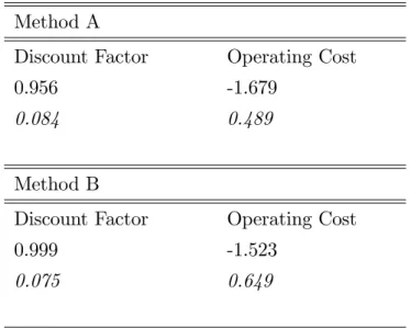
We takeW0 to be known since it cannot be identi…ed jointly withF0, and estimate there remaining
parameters. Since the payo¤ function satis…es Assumption M5 there are two ways to estimate the model. One (Method A) is pro…ling out all the payo¤ parameters using the OLS expression and use grid search to estimate the discount factor. The other (Method B) is to estimate F0 in closed-form
independently …rst before pro…ling out the other payo¤ parameters. Both estimators are expected to be consistent since we know the correct model speci…cation. Otherwise we can perform formal tests to see if they di¤er; see Section 5.2 below. We provide summary statistics for both methods. We consider all three equilibria as enumerated in Pesendorfer and Schmidt-Dengler (2008). We perform
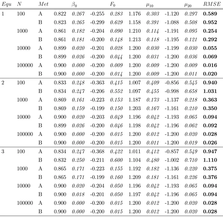
10000 simulations with each sample size, N, of 100;1000;10000 and 100000. We report the mean
Equ N M et 0 F0 10 20 RM SE
1 100 A 0.822 0.267 -0.255 0.283 1.176 0.303 -1.120 0.297 0.589
B 0.823 0.265 -0.299 0.629 1.158 0.391 -1.088 0.508 0.952
1000 A 0.861 0.182 -0.204 0.090 1.210 0.114 -1.191 0.095 0.254
B 0.861 0.181 -0.200 0.148 1.213 0.118 -1.195 0.121 0.292
10000 A 0.899 0.020 -0.201 0.028 1.200 0.030 -1.199 0.030 0.055
B 0.899 0.026 -0.200 0.044 1.200 0.031 -1.200 0.036 0.069
100000 A 0.900 0.000 -0.200 0.009 1.200 0.009 -1.200 0.009 0.016
B 0.900 0.000 -0.200 0.014 1.200 0.009 -1.200 0.011 0.020
2 100 A 0.833 0.248 -0.363 0.415 1.007 0.409 -0.856 0.545 0.940
B 0.834 0.247 -0.206 0.552 1.097 0.455 -0.998 0.658 1.031
1000 A 0.869 0.161 -0.223 0.153 1.187 0.173 -1.137 0.218 0.363
B 0.869 0.159 -0.199 0.150 1.203 0.167 -1.161 0.210 0.350
10000 A 0.900 0.020 -0.203 0.049 1.196 0.042 -1.193 0.065 0.094
B 0.899 0.026 -0.200 0.046 1.198 0.042 -1.196 0.062 0.092
100000 A 0.900 0.000 -0.200 0.015 1.200 0.012 -1.200 0.020 0.028
B 0.900 0.000 -0.200 0.015 1.200 0.011 -1.200 0.019 0.026
3 100 A 0.834 0.247 -0.368 0.422 1.011 0.412 -0.857 0.549 0.947
B 0.832 0.250 -0.211 0.600 1.104 0.480 -1.002 0.710 1.110
1000 A 0.865 0.171 -0.223 0.155 1.192 0.182 -1.136 0.220 0.375
B 0.865 0.171 -0.199 0.160 1.209 0.181 -1.161 0.226 0.376
10000 A 0.900 0.020 -0.204 0.050 1.196 0.042 -1.193 0.065 0.094
B 0.900 0.018 -0.201 0.050 1.197 0.042 -1.196 0.065 0.094
100000 A 0.900 0.000 -0.200 0.015 1.200 0.012 -1.200 0.020 0.028
B 0.900 0.000 -0.200 0.015 1.200 0.012 -1.200 0.020 0.028
Table 1: Summary statistics from estimating 0; F0; 10; 20 using data generated from equilibria 1
to 3 in Pesendorfer and Schmidt-Dengler (2008).
with method A performing marginally better in equilibria 1 and 3, and method B performing mar-ginally better in equilibrium 2. With smaller sample size method B seems to do worse than method A. There also does not seem to be a dominating estimator forF0. Recall that method B requires fewer
assumptions on structure of the model, while method A correctly imposes the remaining parametric structure of the payo¤ function but also has more parameters to estimate simultaneously. Earlier versions of our paper show that when 0 is correctly assumed then the OLS estimator of Sanches et al. (2015) performs better than method B in estimating F0 (using the mean square criterion). We
also …nd that the OLS estimator is inconsistent when incorrect guesses of the discount factor are used.
5.2
Empirical Illustration
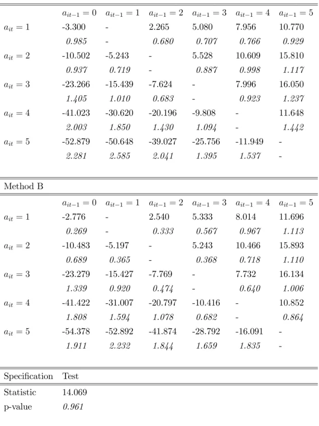
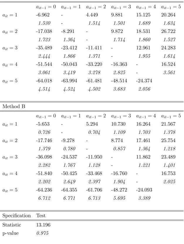
We estimate a simpli…ed version of an entry-investment game based on the model studied in Ryan (2012) using his data. In what follows we provide a brief description of the data, highlight the main di¤erences between the game we model and estimate with that of Ryan (2012). Then we present and discuss our estimates of the primitives.
Data
We download Ryan’s data from the Econometrica webpage.15 There are two sets of data. One
contains aggregate prices and quantities for all the US regional markets from the US Geological Survey’s Mineral Yearbook. The other contains the capacities of plants and plant-level information that Ryan has collected for the Portland cement industry in the United States from 1980 to 1998. Data on plants includes the name of the …rm that owns the plant, the location of the plant, the number of kilns in the plant and kiln characteristics. Following Ryan we assume that the plant capacity equals the sum of the capacity of all kilns in the plant and that di¤erent plants are owned by di¤erent …rms. We observe that plants’ names and ownerships change frequently. This can be due to either mergers and acquisitions or to simple changes in the company name. We do not treat these changes as entry/exit movements. We check each observation in the sample using the kiln information (fuel type, process type, year of installation and plant location) installed in the plant. If a plant changes its name but keeps the same kiln characteristics, we assume that the name change is not associated to any entry/exit movement. This way of preparing the data enables us to match most of the summary statistics of plant-level data in Table 2 of Ryan. Any discrepancies most likely can be attributed to the way we treat the change in plants’ names, which may di¤er to Ryan in a
15
small number of cases.
Dynamic Game
Ryan models a dynamic game played between …rms that own cement plants in order to measure the welfare costs of the 1990 Clean Air Act Amendments (1990 CAAA) on the US Portland cement industry. The decision for each …rm is …rst whether to enter (or remain in) the market or exit, and if it is active in the market then how much to invest or divest. Firm’s investment decisions is governed by its capacity level. The …rm’s pro…t is determined by variable payo¤s from the competition in the product market with other …rms, as well as switching costs from the entry and investment/divestment decisions. There are two action variables in Ryan’s model. One is a binary choice for entry and the other is a continuous level of investment. Past actions are the only observed endogenous state variables in the game. The aggregate data that are used to construct variable pro…ts, through a static Cournot game with capacity constraints between …rms, are treated as exogenous.
We consider a discrete game that …ts the general model description in Section 2. The main departure from Ryan (2012) is that we combine the entry decision along with the capacity level into a single discrete variable. We set the action space to be an ordinal set f0;1;2;3;4;5g, where 0 represents exit/inactive, and the positive integers are ordered to denote entry/active with di¤erent capacity levels. The payo¤ for each …rm has two additive separable components. One depends on the observables while the other is an unobserved shock. The observable component can be broken down to variable and …xed pro…ts. We assume the variable pro…t is determined by the players competing in a capacity constrained Cournot game. The other consists of the switching costs that captures the essence of …rms’ entry and investment decisions. Lastly each …rm receives unobserved pro…t shocks for each action with a standard i.i.d. type-1 extreme value distribution.
Estimation
The period expected payo¤ for each …rm as a function of the observables consists of variable pro…ts, operating costs and switching costs. The variable pro…t is derived from a capacity constrained Cournot game constructed from the same demand and cost functions estimated as in Ryan’s paper. Operating cost enters the payo¤ function additively and is treated as a dynamic parameter to be estimated. These two components are non-zero if ait >0. For the switching costs we normalize the payo¤ for choosing action 0 to be zero. Therefore there are a total of 25 switching cost parameters to be estimated.16
16Ryan (2012) models the switching costs di¤erently. The …xed operating cost is normalized to be zero. Non-zero