REDUCING THE NUMBER OF MEMBERSHIP FUNCTIONS IN LINGUISTIC VARIABLES

(1)

REDUCING THE NUMBER OF MEMBERSHIP

FUNCTIONS IN LINGUISTIC VARIABLES

Margarida Santos Mattos Marques Gomes

Dissertation presented at Universidade Nova de Lisboa, Faculdade de Ciências e Tecnologia in fulfilment of the requirements for the Masters degree in Mathematics

and Applications, specialization in Actuarial Sciences, Statistics and Operations Research

Supervisor: Paula Alexandra da Costa Amaral Jorge Co-supervisor: Rita Almeida Ribeiro

(2)

Acknowledgments

I would like to thank Professor Rita Almeida Ribeiro for inviting me to work at CA3/Uninova in the context of the MODI project and for accepting to co-supervise this thesis. The work developed during this project was the basis of this thesis. Thank you for introducing me to the fuzzy world.

I want to express my gratitude to Professor Paula Amaral, for her excellent guidance and important contribution to overcome some of the difficulties encountered through this thesis.

To all my family and friends, especially my friends at CA3, thank you for the emotional support that gave me strength to finish the thesis.

(3)

Abstract

The purpose of this thesis was to develop algorithms to reduce the number of membership functions in a fuzzy linguistic variable. Groups of similar membership functions to be merged were found using clustering algorithms. By “summarizing” the

information given by a similar group of membership functions into a new membership function we obtain a smaller set of membership functions representing the same concept as the initial linguistic variable.

The complexity of clustering problems makes it difficult for exact methods to solve them in practical time. Heuristic methods were therefore used to find good quality solutions. A Scatter Search clustering algorithm was implemented in Matlab and compared to a variation of the K-Means algorithm. Computational results on two data sets are discussed.

(4)

Resumo

O objectivo desta tese era desenvolver algoritmos para reduzir o número de funções de pertença numa variável linguística. Foram usados algoritmos de agrupamento ou clustering para encontrar grupos de funções de pertença semelhantes. Concentrando a informação dada por um grupo de funções de pertença semelhantes numa nova função de pertença obtém-se um conjunto mais reduzido de funções de pertença que representam o mesmo conceito que a variável linguística original.

Dada a complexidade computacional dos problemas de agrupamento, métodos exactos para a resolução de problemas de programação inteira apenas conseguem encontrar uma solução óptima em tempo útil para pequenas instâncias. Assim, foram usados métodos heurísticos para encontrar boas soluções. Foi implementado em Matlab um algoritmo do tipo Scatter Search e este foi comparado com uma variante do algoritmo K-Means. São apresentados resultados computacionais para dois casos de estudo.

(5)

List of Figures

Figure 1.1: Concepts Short, Medium and Tall represented by Crisp Sets ... 15

Figure 1.2: Concepts Short, Medium and Tall represented by Fuzzy Sets ... 15

Figure 1.3: Fuzzy min ... 17

Figure 1.4: Fuzzy max ... 18

Figure 1.5: Standard fuzzy complement ... 19

Figure 1.6: Precision vs. Significance in the Real World [Mathworks] ... 19

Figure 1.7: Example of fuzzy if-then rule [Mathworks] ... 21

Figure 1.8: Example of fuzzy inference system [Mathworks] ... 22

Figure 1.9: Triangular membership function (a,b,c)(1,3,8) ... 24

Figure 1.10: Symmetrical trapezoidal membership function



a,b,c,d



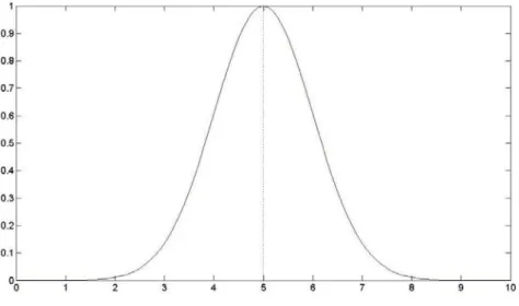
(1,3,6,8) ... 26

Figure 1.11: Gaussian membership function



,

  

 5,1 ... 27

Figure 1.12: Merging trapezoidal membership functions A(1,2,4,6) and B(2,3,5,7) into C(1,2.5,4.5,7). ... 31

Figure 1.13: Merging Gaussian membership functions



₁,₁

 

 5,0.2



and



₂,₂

 

 6,0.4



into



,

 

 5.667,0.3464



... 33

Figure 2.1: Diagram of Clustering Algorithms [Gan, Ma et al. 2007] ... 36

Figure 2.2: Dendogram ... 37

Figure 2.3: Example of single-link method using a MST: (a) distance matrix; (b) weighted graph; (c) MST; (d) Dendogram ... 45

Figure 2.4: Example of a Linguistic Variable with three fuzzy sets ... 53

Figure 4.1: Scatter Search Algorithm ... 68

Figure 4.2: Linguistic Variable Radius ... 78

Figure 4.3: Linguistic Variable Texture ... 78

Figure 4.4: Linguistic Variable Perimeter ... 79

Figure 4.5: Linguistic Variable Area ... 79

Figure 4.6: Linguistic Variable Smoothness ... 80

Figure 4.7: Linguistic Variable Compactness ... 80

Figure 4.8: Linguistic Variable Concativity ... 81

Figure 4.9: Linguistic Variable Concave Points ... 81

Figure 4.10: Linguistic Variable Symmetry ... 82

Figure 4.11: Linguistic Variable Fractal Dimension ... 82

Figure 4.12: Evaluation measure I using K-means++ for 1K568, linguistic variable Radius ... 83

Figure 4.13: Evaluation measure I using K-means++ for 1K500(zoom in of previous plot) 1 K568, linguistic variable Radius ... 84

Figure 4.14: Evaluation measure I using K-means++ for 1K568, linguistic variable Texture ... 84

Figure 4.15: Evaluation measure I using K-means++ for 1K500(zoom in of previous plot), linguistic variable Texture ... 85

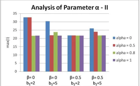
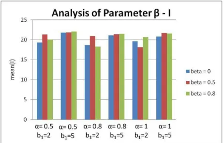
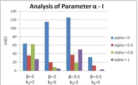
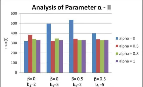
Figure 4.16: Influence of  in fitness function I standard deviation ... 86

Figure 4.17: Influence of  in best results obtained for fitness function I ... 87

Figure 4.18: Influence of  in mean results for fitness function I ... 87

(8)

Figure 4.20: Influence of b₁ in mean results for fitness function I ... 89

Figure 4.21: Influence of b₁ in execution time ... 89

Figure 4.22: Influence of Improvement Method in mean ... 90

Figure 4.23: Influence of Improvement Method in execution time ... 91

Figure 4.24: Best Results for Linguistic Variable Radius ... 93

Figure 4.25: Best Results for Linguistic Variable Texture ... 94

Figure 4.26: Best Results for Linguistic Variable Perimeter ... 95

Figure 4.27: Best Results for Linguistic Variable Area ... 96

Figure 4.28: Best Results for Linguistic Variable Smoothness... 97

Figure 4.29: Best Results for Linguistic Variable Compactness ... 98

Figure 4.30: Best Results for Linguistic Variable Concativity ... 99

Figure 4.31: Best Results for Linguistic Variable Concave Points ... 100

Figure 4.32: Best Results for Linguistic Variable Symmetry ... 101

Figure 4.33: Best Results for Linguistic Variable Fractal Dimension ... 102

Figure 4.34: Linguistic Variable A2 ... 104

Figure 4.40: Evaluation measure I using K-means++ for 1K665, linguistic variable A2 ... 108

Figure 4.41: Evaluation measure I using K-means++ for 1K150(zoom in of previous plot), linguistic variable A2 ... 108

Figure 4.42: Evaluation measure I using K-means++ for 1K665, linguistic variable A3 ... 109

Figure 4.43: Evaluation measure I using K-means++ for 1K150 (zoom in of previous plot), linguistic variable A3 ... 109

Figure 4.44: Influence of  in fitness function I standard deviation ... 110

Figure 4.45: Influence of  in best results obtained for fitness function I ... 111

Figure 4.46: Influence of  in mean results for fitness function I ... 111

Figure 4.47: Influence of  in mean results for fitness function I ... 112

Figure 4.48: Influence of b₁ in mean results for fitness function I ... 112

Figure 4.49: Influence of b₁ in execution time ... 113

Figure 4.50: Influence of Improvement Method in mean ... 113

Figure 4.51: Influence of Improvement Method in execution time ... 114

Figure 4.52: Best Results for Linguistic Variable A2 ... 115

Figure 5.1: MODI drill station ... 123

Figure 5.2: ExoMars Rover (courtesy of ESA [ESA 2008]) ... 123

Figure 5.3: Example of linguistic variable – Rotational Voltage ... 126

Figure 5.4: Original algorithm [Setnes, Babuska et al. 1998] ... 128

Figure 5.5: Example of model error ... 129

(9)

Figure 5.8: Final algorithm – bestP ... 133 Figure 5.9: Original input linguistic variables (except set points) ... 135 Figure 5.10: Evolution of performance measure Fduring the algorithm – Rotation Current ... 136 Figure 5.11: Evolution of performance measure Fduring the algorithm – Rotation Voltage ... 137 Figure 5.12: Evolution of performance measure Fduring the algorithm – Rotation Speed ... 137 Figure 5.13: Evolution of performance measure Fduring the algorithm – Thrust .... 138 Figure 5.14: Evolution of performance measure Fduring the algorithm – Torque ... 138 Figure 5.15: Evolution of performance measure Fduring the algorithm –

Translational Voltage ... 139 Figure 5.16: Evolution of performance measure Fduring the algorithm –

Translational Current ... 139 Figure 5.17: Evolution of performance measure Fduring the algorithm –

(10)

List of Tables

Table 3.1: Computational Results ... 61

Table 4.1: K-Means++ vs Scatter Search (best results) ... 92

Table 4.2: K-Means++ vs Scatter Search (best results) ... 115

Table 5.1: MODI Confusion Matrix ... 126

Table 5.2: Number of membership functions before and after optimization ... 140

(11)

Introduction

In human reasoning many concepts are not crisp in the sense of being completely true or false, instead they can be interpreted in a more qualitative way. In everyday life we use concepts like tall, small, fast, slow, good, bad … that are difficult to translate numerically. Classical logic and inference have been insufficient to deal with these apparently vague concepts. Although humans reason with these concepts in a natural way on a daily basis, our search for scientific knowledge has lead us to address the problem of representing these concepts in a more systematic and precise way. As Engelbrecht [Engelbrecht 2002] states, “In a sense, fuzzy sets and logic allow the modelling of common sense”.

Since 1965, when Zadeh first formalized the concept of fuzzy set [Zadeh 1965], the field of fuzzy logic and approximate reasoning has attracted the interest of the scientific community. Fuzzy set theory and fuzzy logic concepts have been applied in almost all fields, from decision making to engineering [Costa, Gloria et al. 1997; Ross 2004], from medicine [Adlassnig 1986 ] to pattern recognition and clustering [Nakashima, Ishibuchi et al. 1998].

In engineering, fuzzy logic has been used, for instance, in monitoring and classification applications [Isermann 1998; Ribeiro 2006]. The main goal when constructing a fuzzy monitoring system is to develop a fuzzy inference system (FIS) [Lee 1990a; Lee 1990b] to monitor certain variables and warn decisors (or an automatic system) when variables behaviour is not correct, so that they can intervene. For the development of monitoring systems, in general, a formal and precise mathematical understanding of the underlying process is usually needed. These mathematical models may become too complex to formalize or to implement, reducing the advantage of an automatic and independent system over a human expert. Once again, fuzzy knowledge can be used to overcome this problem, modelling complex systems by mimicking human thinking.

(12)

preferences and choices of decision makers have many uncertainties and are better represented through a fuzzy number. Although crisp decision models do exist, more and more papers and books propose the use of fuzzy sets and fuzzy models to deal with the underlying uncertainty [Anoop Kumar and Moskowitz 1991; Lai and Hwang 1994; Ribeiro 1996; Ross 2004].

The main idea when choosing a fuzzy model over a classical one is to obtain models that are less complex and easy to interpret. The trade off between interpretability and precision must be studied for each application. To achieve such interpretability, it is desirable that the linguistic variables in a fuzzy model [Zadeh 1975] are as intuitive as possible. This in addition to a search for computationally efficient models motivated the research of this master thesis. When linguistic variables are constructed directly from expert knowledge its interpretability is usually clearer. This is not the case when an automatic procedure is used to create the membership functions of a certain linguistic variable or when membership functions represent a single sample from a large data base. As an example consider a fuzzy set used to represent an agent preference between two alternatives and suppose the number of agents involved in the process to be modelled is considerably large.

The purpose of this thesis is to develop algorithms to reduce the number of membership functions in a linguistic variable. The problem of reducing the amount of data to be analysed, while maintaining as most information as possible from the original data, is not exclusive from fuzzy domains. Large crisp data sets often have to be clustered to become treatable [Hartigan 1975; Murtagh 1983; Everitt, Landau et al. 2001; Gan, Ma et al. 2007]. Clustering data corresponds to finding natural groups of data that represent similar objects. The same approach can be used to reduce the number of membership functions in linguistic variables. We start by identifying clusters of similar membership functions. If each cluster of membership functions can

be “summarized” into a new membership function, we obtain a new and smaller set

of membership functions that approximately represents the same concept as the initial linguistic variable. This will be the basic approach that will be developed during this thesis. The problem of reducing the number of membership functions in linguistic variables will be formulated as a clustering problem. Resulting clusters of

(13)

In Chapter 1 theoretical background that is needed to understand following development is presented. An introduction to fuzzy logic and fuzzy inference systems is described. Similarity measures and merging methods that will be used to reduce the number of membership functions in linguistic variables are also introduced.

Since, as stated before, the problem of reducing the number of membership functions in a linguistic variable can be stated as a clustering problem, Chapter 2 will present different approaches to the clustering problem in statistics and optimization and the state of the art. Also, some possible formulations to the clustering problem will be discussed.

The complexity of clustering problems makes it difficult for exact methods to solve them in practical time. Exact methods can only find an optimal solution in a reasonable amount of time for very small data sets, especially if the number of clusters is unknown. However, before deciding for heuristic methods, it is important to use exact methods to better understand the complexity of the problem at hands. Since it was never the purpose of this thesis to solve these problems through exact methods, Chapter 3 gives only a brief introduction to some of the exact methods used for combinatorial and integer programming.

When finding optimal solutions through exact procedures is too time consuming, it is still usually possible to find good quality solutions in a reasonable amount of time, using heuristic methods that take advantage of the problem structure to achieve good solutions (not necessarily optimal) in less computational time. Both a heuristic and a metaheuristic to solve the automatic clustering problem were implemented in Matlab. Chapter 4 describes these algorithms and presents computational results on two case studies. In both case studies several linguistic variables are pruned. These linguistic variables could later be used in a fuzzy inference system or any other fuzzy model. The model would be constructed taking into account the already clustered membership functions instead of the original ones.

(14)

of project “MODI – Simulation of a Knowledge Enabled Monitoring and Diagnosis

Tool for ExoMars Pasteur Payloads”[CA3 2006; Jameaux, Vitulli et al. 2006; Santos, Fonseca et al. 2006], a CA3 – UNINOVA project for the European Space Agency [ESA] Aurora programme [ESA 2008]. In this project two inference systems were constructed: one for monitoring exploratory drilling processes and another capable of detecting the type of terrain being drilled. These systems were automatically constructed using data collected from sensors while drilling in different scenarios. With these systems already constructed, the task was to reduce the number of membership functions in its linguistic variables without losing performance. This project was on the origin of the development of the ideas presented in this thesis. The contribution to this project can also be found in [Gomes, Santos et al. 2008]. This paper summarizes the main results obtained when reducing the number of

membership functions of MODI’s linguistic variables and was presented at the Eight International Conference on Application of Fuzzy Systems and Soft Computing (ICAFS-2008) in September 2008 in Helsinki, Finland.

(15)

Chapter 1. Preliminaries

In this Chapter we present the background on fuzzy set theory necessary to understand the results presented later.

Sections 1.1 and 1.2 introduce the main concepts of fuzzy logic and fuzzy inference systems. Formal definitions of the concepts of linguistic variable, fuzzy set, membership function and the most used operations on fuzzy sets are given. A description of the structure of a fuzzy inference system and of its underlying modules is also presented.

In section 1.3, analytical and p

R representations of some of the most common types of membership functions - triangular, trapezoidal and Gaussian membership functions – are introduced.

The notion of similarity or proximity between membership functions will be the main idea underneath the algorithms for reducing the number of membership functions in linguistic variables. Section 1.4 describes these concepts and presents the measures of proximity of fuzzy sets that will be used. After identifying the most similar membership functions, these will be merged to give rise to a new set of membership functions simultaneously as small and as representative of the original linguistic variable as possible. Section 1.5 presents some membership functions merging methods.

1.1 Fuzzy Logic

(16)

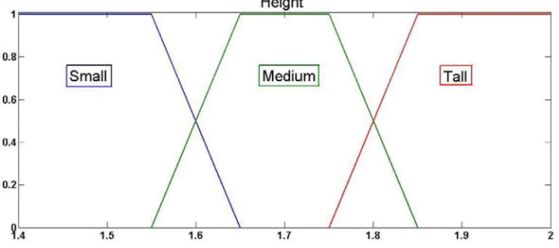
Figure 1.1: Concepts Short, Medium and Tall represented by Crisp Sets

This does not accurately represent human reasoning. In our mind, the frontier between these sets is not as well defined as in Figure 1.1. These concepts are better represented by fuzzy sets [Zadeh 1965], as in Figure 1.2. This representation allows for an individual to be considered simultaneously short and medium or medium and tall, with different degrees of membership. The definition of fuzzy set is given bellow.

Figure 1.2: Concepts Short, Medium and Tall represented by Fuzzy Sets

Definition 1.1 [Zimmermann 1990] - If X is a collection of objects denoted

generically by x then a fuzzy set A~ in X is a set of ordered pairs:







x x x X



A , A( ) : 

~ _ _(1.1)

where ~(x)

A

 is called the membership function or grade of membership of x in A~ which mapsX to the membership space M . The range of the membership function is

B

A C

D Short

G E

(17)

a subset of nonnegative real numbers whose supremum is finite. Usually M is the real interval

 

0,1 .

♦

The representation of some common types of membership functions will be further presented in the next section.

Zadeh [Zadeh 1975] defines a linguistic variable as a quintuple )

, , ), ( ,

(x T x U G M in which x is the name of the variable; T(x)is the term set of x, that

is, the collection of its linguistic values; U is a universe of discourse; G is a syntactic rule which generates the terms in T(x); and M is a semantic rule which associates with each linguistic value T(x) its meaning, M(X), where M(X)denotes a subset of U.

The fuzzy sets in Figure 1.2 represent a linguistic variable Height.

T-norms and t-conorms generalize the idea of intersection and union of sets to fuzzy set theory.

Definition 1.2 [Klir and Yuan 1995] – A t-norm is a function t:

     

0,1  0,1  0,1

satisfying the following properties:

Boundary Condition: t(a,1)a (1.2)

Monotonicity: t(a,b)t(a,c) if bc (1.3) Commutativity: t(a,b)t(b,a) (1.4) Associativity: t(a,t(b,c))t(t(a,b),c) (1.5)

♦

Definition 1.3 [Klir and Yuan 1995] – A t-conorm or s-norm is a function

     

0,1 0,1 0,1

:  

u satisfying the following conditions:

(18)

Monotonicity: u(a,b)u(a,c) if bc (1.7) Commutativity: u(a,b)u(b,a) (1.8) Associativity: u(a,u(b,c))u(u(a,b),c) (1.9)

♦

The fuzzy minimum and the fuzzy maximum, defined bellow, are the most used t-norms and t-conorms. Examples of these operators can be found in Figure 1.3 and Figure 1.4, respectively.

Definition 1.4 [Klir and Yuan 1995] – Given two fuzzy sets A and B, their standard

intersection, AB, and standard union, AB, also known as fuzzy minimum and fuzzy maximum, are defined for all xX by the equations:



( ), ( )



min

) )(

(AB x  A x B x (1.10)



( ), ( )



max

) )(

(AB x  A x B x (1.11)

♦

(19)

Figure 1.4: Fuzzy max

To generalize the concept of negation, complement operators are used. The membership function of a fuzzy set A represents, for each x in its universe of discourse, the degree to which x belongs to A. The membership functions of the complement of A represents the degree to which x does not belong to A.

Definition 1.5 [Klir and Yuan 1995] – A complement of a fuzzy set A is specified by

a function c:

   

0,1  0,1 satisfying the following properties [Klir and Yuan 1995]:

Boundary Conditions: c(0)1; c(1)0 (1.12) Monotonicity: c(a)c(b) if ab (1.13)

♦

The standard complement is defined bellow and exemplified in Figure 1.5.

Definition 1.6[Klir and Yuan 1995] - The standard complement, A, of a fuzzy set A

with respect to the universal set X is defined for all xX by the equation:

) ( 1 )

(x A x

A   (1.14)

(20)

Figure 1.5: Standard fuzzy complement

1.2 Fuzzy Inference Systems

(21)

There are two main kinds of fuzzy inference systems, Mamdani and Sugeno [Lee 1990a; Lee 1990b]. The knowledge base of a Mamdani inference system contains rules where both the antecedents and the consequents are fuzzy sets. Sugeno inference systems, on the other hand, use rules with fuzzy antecedents and crisp consequents. In this thesis only Mamdani inference systems will be used but the ideas and algorithms developed can also be used in Sugeno inference systems.

Fuzzy if-then rules used in Mamdani inference systems are expressions of the type [Ross 2004]:

“if x is A then y is B”

where A and B are fuzzy sets, “x is A” is called the antecedent and “y is B” is called the consequent of the rule.

The antecedent part of the rule can have multiple parts connected by fuzzy operators, typically t-norms and t-conorms giving meaning to the linguistic

expressions “and” and “or” respectively. The consequent can have multiple parts representing distinct conclusions that can be inferred from the given antecedent. The firing level or firing strength of the rule is the degree to which the antecedent part of the rule is satisfied.

(22)

Figure 1.7: Example of fuzzy if-then rule [Mathworks]

(23)

Figure 1.8: Example of fuzzy inference system [Mathworks]

(24)

service=3 and food=8. Aggregating these three fuzzy sets, the fuzzy set in the bottom right of Figure 1.8 is obtained. In this example the centre of area or centroid defuzzification method, defined by (1.15), is used and a tip of 16.7% is recommended.

Definition 1.7 [Klir and Yuan 1995] - Consider a fuzzy set A with membership

function _A:X 

 

0,1. The centre of area or centroid defuzzification method returns the value d_CA(A) within X for which the area underneath the graph of membership function A is divided into two equal subareas. This value is given by the following

expression: dx x dx x x A d X A X A CA ) ( ) ( ) (



    (1.15) ♦

1.3 Representation of Membership Functions

Some types of membership functions can be mapped to p

R , where p is the number of parameters of that family of membership functions and each dimension represents a different parameter. In this section both analytical and p

R representations of some of the most common types of membership functions are presented.

1.3.1 Triangular Membership Functions

Definition 1.8 - A triangular membership function is given by the analytical

(25)





                  otherwise , 0 , , , ,

, b x c

b c x c b x a a b a x x c b a  (1.16)

where a,band c correspond to the x-axis coordinates of the vertices of the triangle,

as in Figure 1.9.

♦

There are several possibilities for mapping these membership functions into

3 , 2 , p

Rp . For instance, for p3 we can consider a vector with the x-axis coordinates of the vertices of the triangle,



a,b,c



, or a vector



b,L,R



where

a b

L  

 and _R cb represent its left and right spreads, respectively. This way

we define a mapping between the family of triangular membership functions and 3 R . If we only consider symmetrical membership functions, i.e., if_L _R  , we can use a pair

 

b, to represent a membership function of this family. In this way the

mapping can be done in 2 R .

(26)

1.3.2 Trapezoidal Membership Functions

Definition 1.9 - A trapezoidal membership function is given by the analytical

expression:





                    otherwise , 0 , , , 1 , , , , d x c c d x d b x a a b a x c x b x d c b a  (1.17)

where a,b,cand dcorrespond to the x-axis coordinates of the vertices of the

trapezoid, as in Figure 1.10.

♦

Similarly to the case of triangular membership functions, we can now map the family of trapezoidal membership functions to 4

R and R3(symmetric trapezoidal). We can consider a vector with the x-axis coordinates of the vertices of the trapezoidal,



a,b,c,d



, to map this family of membership functions to R4 and if we only consider

symmetrical membership functions, i.e., if

2 2

c b d a _ 

, we can use a vector



m,,



,

where 2 2 c b d a

m    ,  cb and  da, to represent a membership function

(27)

Figure 1.10: Symmetrical trapezoidal membership function



a,b,c,d



(1,3,6,8)

1.3.3 Gaussian Membership Functions

Definition 1.10 – A Gaussian membership function is given by the analytical

expression:

 _2

   x

e (1.18)

where  and  are the mean and spread of the Gaussian function.

♦

The mapping of this family of membership functions to _R2_{is straightforward}

(28)

Figure 1.11: Gaussian membership function



,

  

 5,1

1.4 Proximity Measures between Membership Functions

As stated in the introduction of this Chapter, the notion of similarity or proximity between membership functions will be the main idea underneath the algorithms for reducing the number of membership functions in linguistic variables. When faced with the problem of reducing the number of terms in linguistic variables, we intuitively think of joining or merging membership functions that are somehow similar. For crisp data sets, a similar idea is the foundation of cluster analysis. Clusters are groups of objects that are similar according to some proximity measure [Hartigan 1975]. The problem presented in this thesis can then be approached as a clustering problem where the objects are membership functions and suitable proximity measures are used.

(29)

One of the most used set-theoretical similarity measures, the fuzzy Jaccard index or Jaccard similarity measure [Miyamoto 1990], is defined by:





B A B A B A S_J    , (1.19)

where 



U C x dx

C| ( )

|  and (,) is a pair of fuzzy t-norms

 

 and t-conorms ().

An overview of some similarity measures for comparing fuzzy sets can be found in [Chen, Yeh et al. 1995]. The Jaccard similarity measure will be used in the algorithms presented in Chapter 5, but other similarity measures could also be used. For instance, since in Chapter 5 only trapezoidal membership functions are used, the following two similarity measures used for comparing trapezoidal fuzzy sets could be considered.

The first one can be calculated by the following expression [Chen 1996]:

4 | | 1 ) , ( 4 1



    i i i C b a B A S (1.20)

where A(a₁,a₂,a₃,a₄) and B(b₁,b₂,b₃,b₄).

The second one was proposed by Shi-Jay Chen and Shyi-Ming Chen [Chen and Chen 2008] and is given by:

) , max( ) , min( |) | 1 ( 4 | | 1 ) , ( ( , ) 4 1        _ _ _ _             _  



B A B A S S B B A i i i SCGM y y y y x x b a B A

S A B (1.21)

where         0 if , 0 0 if , 1 ) , ( B A B A B A S S S S S S B (1.22) 1 4 a a

S_A   (1.23)

1 4 b b

(30)

and (xA,yA) and ( , )

 

B

B y

x are the centre of gravity points of A and B, respectively. These points can be easily determined by the simple centre of gravity method (SCGM) [Chen and Chen 2008], using the following expressions:

              4 1 4 1 1 4 2 3 , 2 1 , 6 2 a a if a a if a a a a

y_A (1.25)

2 ) 1 )( ( )

( ₃ ₂ ₄ ₁ 



 _ A     A

A y a a a a y x (1.26)

In the previous section it was shown how the most used families of membership functions can be mapped to p

R . By mapping a membership function to

p

R the problem to be addressed becomes equivalent to finding clusters given a data set in p

R , provided that we are considering linguistic variables where all membership functions belong to the same family, which is usually the case. Therefore, the proximity measures used for comparing objects in p

R can also be used to compare membership functions of the same family. For instance, the Euclidean Distance given by (1.27) can be used to compare two membership functions of the same family,



a ap



A ₁,, and B



b1,,bp



, represented in p

R . This will be done in the algorithms presented in Chapter 4 where the problem of reducing the number of membership functions in linguistic variables will be approached by clustering the vectors of parameters representing the membership functions.

(31)

1.5 Merging Membership Functions

In this section we discuss some methods on how to merge membership functions to reduce the number of membership functions in a linguistic variable, by using the concept of similarity. This section is not intended as an overview of the possible methods for merging membership functions since these methods could vary according to several factors: the type of membership functions being merged, the algorithms in use, the context of the problem, among others.

Membership functions of the types referred in section 1.2 will be considered, since these are the most used ones. Also, throughout this thesis, it will be assumed that all membership functions of a certain linguistic variable to be pruned share the same type (either triangular or trapezoidal) and that the merging of two membership functions should yield a new membership function of the same type as the original ones. This simplification does not change the nature of the problem and the algorithms that will be use to solve it are as general as possible. If one of these conditions fails we only have to redefine the way two membership functions are merged but the algorithms still apply.

1.5.1 Merging Trapezoidal Membership Functions

Given two trapezoidal membership functions A(a1,a2,a3,a4) and )

, , ,

(b1 b2 b3 b4

B , merging them using the method proposed in [Setnes, Babuska et al. 1998] gives a new trapezoidal membership function C(c1,c2,c3,c4) where:



1 1



1 min a ,b

c  (1.28)



2



2 2

2

2 a 1 b

c    (1.29)



3



3 3

3

3 a 1 b

c    (1.30)



4 4



4 max a ,b

(32)

The parameters ₂ and ₃belong to the interval

 

0,1. These parameters allow weighting the importance of A and B in the final membership C. In subsequent chapters this operator will be used with 2 3 0.5. See for instance Figure 1.12, which shows the trapezoidal membership functions A(1,2,4,6) and B(2,3,5,7) combined into C(1,2.5,4.5,7). Notice that (1.28) and (1.31) guarantee that the same

“coverage” as A and B, i.e., points with positive membership in either A or B will still have positive membership in C. This might be crucial for some applications.

Figure 1.12: Merging trapezoidal membership functions A(1,2,4,6) and B(2,3,5,7) into C(1,2.5,4.5,7).

In the previous merging method only two membership functions are merged at a time. When merging more than two membership functions at a time, a generalization of this method was used. Given n trapezoidal membership functions



a b c d



i n

Ti  _i, _i, _i, _i , 1,, , these will be simultaneously merged into a membership function T 



a,b,c,d



, i1,,n where:

i n

i a

a , , 1

min





 (1.32)





 n

i i

b n b

1

(33)



  n i i c n c 1 1 _(1.34) i n i d d , , 1 max    (1.35)

1.5.2 Merging Triangular Membership Functions

It is straightforward to adapt the previous methodology to the case of triangular membership functions. Considering that a triangular membership function is a trapezoidal membership function with bi ci Given n triangular membership

functions Si 



a_i,b_i,d_i



, i1,,n, these will be simultaneously merged into a membership function S 



a,b,d



, i1,,n where:

i n i a a , , 1 min    (1.36)



  n i i b n b 1 1 _(1.37) i n i d d , , 1 max    (1.38)

1.5.3 Merging Gaussian Membership Functions

In [Song, Marks et al. 1993] the fusion of two Gaussian membership functions with parameters



1,1



and



2,2



is a Gaussian membership function with

parameters



,



defined by the following equations. See for instance Figure 1.13.

(34)

2 1 3 2 3 1 2         (1.40)

Figure 1.13: Merging Gaussian membership functions



₁,₁

 

 5,0.2



and



2,2

 

 6,0.4



into



,

 

 5.667,0.3464



We can extend this method by defining the merge of n Gaussian membership

functions with parameters



i,i



, i1,,n as by the pair



,



, where:



   _n i i n i i i 1 1     (1.41)



   _n i i n i i 1 1 3 2    (1.42)

1.6 Summary

(35)

are the basic concepts of fuzzy logic and inference systems. Analytical and p

(36)

Chapter 2. A Clustering Problem Approach

As stated in the introduction, the problem of reducing the number of membership functions in linguistic variables can be formulated as a clustering problem. We need to identify groups of similar membership functions and merge them. As a result, we should obtain a smaller set of membership functions capable of approximately represent the initial linguistic variable.

In section 2.1 the clustering problem will be introduced. Section 2.2 will present the state of the art and finally in section 2.3 some integer programming formulations for the clustering problem will be given.

2.1 The Clustering Problem

There is no uniform formal definition for data clustering. The task of defining the meaning of clustering have been pointed out as a difficult one by several authors [Everitt, Landau et al. 2001; Estivill-Castro 2002]. In [Gan, Ma et al. 2007] the following informal definition can be found:

“Data clustering (or just clustering), also called cluster analysis, segmentation analysis, taxonomy analysis, or unsupervised classification, is a method of creating groups of objects, or clusters, in such a way that objects in one cluster are very similar and objects in different clusters are quite distinct.”

(37)

this problem as a fuzzy clustering problem by allowing membership functions to belong to more than one cluster and defining appropriate membership function merging techniques is a possibility to be studied in the future.

Figure 2.1: Diagram of Clustering Algorithms [Gan, Ma et al. 2007]

2.2 State of the Art

As stated in the previous section, there is no unique definition of clustering. Appropriate criteria for clustering have to be chosen for each application, according to the type of groups to be found in data. This partially explains the existing diversity of clustering algorithms [Estivill-Castro 2002]. Given this diversity, this state of the art will not be exhaustive in describing all the existing methods. Some more extensive reviews can be found in [Sokal and Sneath 1963; Hartigan 1975; Rijsbergen 1979; Jain and Dubes 1988; Kaufman and Rousseeuw 1990; Jain, Murty et al. 1999; Everitt, Landau et al. 2001; Engelbrecht 2002; Mirkin 2005; Gan, Ma et al. 2007].

(38)

Hierarchical methods return a hierarchy or set of nested partitions while partition methods return a single partition of the data.

The next subsections will present the main ideas of hierarchical methods (section 2.2.1), classical partition methods (section 2.2.2), graph based methods (section 2.2.3), metaheuristics (section 2.2.4) and other clustering methods (section 2.2.5).

2.2.1 Hierarchical Methods

As stated before, hierarchical methods return a hierarchy or set of nested partitions, as depicted in Figure 2.2. Agglomerative hierarchical algorithms start with each data point in a different cluster and proceed by merging clusters, according to some criterion, until there is only one cluster containing all data points in the data set. Divisive hierarchical algorithms start with one cluster containing all data points and proceed by splitting clusters until each data point is in a different cluster.

Figure 2.2: Dendogram

(39)

1. Compute the proximity matrix containing the distance between each pair of data points. Treat each data point as a cluster;

2. Find the most similar pair of clusters using the proximity matrix and merge them into one cluster;

3. Update the proximity matrix to reflect the merging operation in 2; 4. If all data points are in one cluster, stop. Otherwise, go to step 2.

Different algorithms can be developed according to the way the proximity measure is updated in step 3. The most used are the single-link, complete link and

Ward’s methods [Jain, Murty et al. 1999].

The single-link method, also known as nearest neighbour method and minimum method, was first introduced by [Florek, Lukaszewicz et al. 1951] and then independently by [McQuitty 1957] and [Sneath 1957]. Let C₁ and C₂ be two clusters and d

 

, a distance measure between two points. In the single-link method, the

distance between C₁ and C₂, also referred to as linkage function, is given by:



C C



d

 

x y D

C y C

x min ,

,

2 1,

2

1  _ _ (2.1)

The complete-link [King 1967], also known as farthest neighbour method, updates the proximity measure using the following expression, using the same notation as in (2.1).



C C



d

 

x y D

C y C

xmax ,

,

2 1,

2

1  _ _ (2.2)

The Ward’s method [Ward Jr. 1963; Ward Jr. and Hook 1963], also known as minimum-variance method, aims at forming partitions Pn,,P1 of the original data

(40)



  K i i C ESS ESS 1 ) ( (2.3) where





 





 



    C x T C x C x C

ESS( )   (2.4)

and



  X x x C X) 1 (

 (2.5)

At each step of the Ward’s method the two clusters whose fusion results in the

minimum increase in loss of information are merged. The linkage function is computed as the increase in ESS after merging two clusters, i.e.:



C₁,C₂



ESS



C₁C₂



ESS

 

C₁ ESS

 

C₂

D    (2.6)

where C₁C₂ denotes the cluster resulting from merging C₁ and C₂.

Other linkage functions are described in [Hartigan 1975; Everitt, Landau et al. 2001; Gan, Ma et al. 2007]. In [Kuiper and Fisher 1975] a comparison of several hierarchical clustering algorithms is done using the Monte Carlo method.

As stated before, divisive hierarchical algorithms proceed the opposite way of the agglomerative algorithms. We start with one cluster containing all data points and proceed by splitting clusters until each data point is in a different cluster. Since given

(41)

To illustrate divisive hierarchical clustering algorithms we will consider the DIANA (DIvisive ANAlysis) algorithm proposed by [Kaufman and Rousseeuw 1990].

For a given distance measure d(,), the diameter of a cluster C is given by:

 

max ( , ) , d x y C

Diam

C y

x 

 (2.7)

Denote the average dissimilarity from a point x to the points in a set S by

 

x S

D , , i.e.,

 

_

 





S y

y x d S S x

D , 1 , (2.8)

In each step of the DIANA algorithm, the cluster with largest diameter, C

(C 2), is split into two subclusters, A and B. These subclusters are determined by the following procedure:

1. Do AC and B

 

;

2. Do z argmax



D



x,A\

 

x



,xA



;

3. Move point z from A to B, i.e., AA\

 

z and BB

 

z ; 4. Do z argmax



D



x,A\

 

x



D

 

x,B ,xA



;

5. If D



z,A\

 

z



D

 

z,B 0 then move point z from A to B, i.e., AA\

 

z

and BB

 

z , and return to 4. Otherwise stop the procedure, returning

A and B.

(42)

Generally, hierarchical methods have a complexity of ( 2) n

O for memory space and O(n3) for CPU time [Hartigan 1975; Murtagh 1983], n being the number of points to be clustered. Therefore, they become impractical for large data sets.

2.2.2 Classical Partition Clustering Methods

Unlike hierarchical methods, partition methods create a single partition of the data points.

The most known partition method is the K-Means algorithm [McQueen 1967]. This algorithm is a centre-based method. Each cluster is represented by a centre and the corresponding clusters have convex shapes. The algorithm starts by choosing initial K cluster centres from the original data. After the initialization, a partition of the data is determined by assigning each point to the cluster with closest centre. After this assignment the centroids of each cluster are calculated according to the following expression: K i x C c i C x i

i , 1, ,

1   



 (2.9)

where ci is the centre of cluster Ci.

Then the points are reassigned to the clusters regarding the closeness to the centroids. Again, the centroids are recalculated and the algorithm proceeds in the same way until some stopping criterion is met. Usually the algorithm will proceed until the cluster centroid and partition no longer change or until a predefined number of iterations is reached. This way the K-Means algorithm is a heuristic method that tries to minimize the sum of squared distances from each point to its cluster centre. The number of clusters K is determined by the user a priori. In practice, if the user can not identify the correct number of clusters, the algorithm is run for a certain range for the number of clusters, i.e. K



Kmin,,Kmax



, and the best configuration found,

(43)

Many variations of the original K-Means algorithm have been developed. Some try to improve the efficiency of the algorithm by reducing the computational effort demanded by the algorithm [Tapas, David et al. 2002]. Others differ from the original algorithm in the way the initial cluster centres are chosen, as is the case of the algorithm presented in [David and Sergei 2007] called K-Means++ that will be further discussed in section 4.1. Some allow merging or splitting clusters according to centres distances or cluster within variance [Ball and Hall 1965].

Another widely used partition method is the Expectation Maximization Algorithm (EM) [Dempster, Laird et al. 1977], a model based clustering algorithm. In model based clustering it is assumed that the data comes from a certain mixture of

distributions





 K

k

k f x a

p x f 1 ) , ( ) (       _

_

_  K k k k p p 1 1 ,

0 , with each component f(x,ak) representing a different cluster, where f(x,ak) is a family of density functions over x and ak is the parameter vector that identifies a particular density from that family.

Model based clustering algorithms try to optimize the fit between the data and the proposed model.

To estimate the individual cluster parameter the EM algorithm uses the maximum likelihood approach. The logarithm of the likelihood of the observed data given by (2.10) is maximized under the assumption that the data comes from a mixture of distributions.





      



  N i K k k i

kf y a

p L

1 1

,

log (2.10)

Maximization of (2.10) can be reformulated as the maximization of (2.11).









         N i N i K k ik ik K k k i ik N i K k k

ik p g f y fa g g

g L

1 1 1 1

(44)

and K and N are the number of clusters and data points, respectively.

The EM algorithm can then be summarized in the following way [Mirkin 2005]:

1. Start with any initial values of the parameters p_k,a_k and gik,

N

i1,, , k 1,,K;

2. (E-step) Given p_k and a_k estimate g_ik;

3. (M-step) Given gik find pk and ak maximizing (2.11);

4. Repeat steps 2 and 3 until there is no change in the parameter values (or the absolute difference is below some previously defined threshold).

2.2.3 Graph Based Methods

The relationship between graph theory and the clustering problem has been discussed by [Wirth, Estabrook et al. 1966; Jardine and Sibson 1968; Gower and Ross 1969; Hubert 1974; Hansen and Delattre 1978], among other authors. Algorithms that take advantage of the graph theoretical properties of data are called graph based methods.

The single-link and complete-link hierarchical methods discussed in section 2.2.1 can be approached from a graph theoretical view. More computationally efficient algorithms for single and complete link hierarchical methods than the ones already presented are described in [Gower and Ross 1969; Hansen and Delattre 1978; Jain and Dubes 1988].

A minimum spanning tree (MST) of a connected, undirected, weighted graph is a subgraph that connects all its edges without cycles (tree) with minimum weight. Several methods for finding a minimum spanning tree of a graph have been developed [Kruskal 1956; Prim 1957]. In [Jain and Dubes 1988] the following algorithm for the single-link method using a minimum spanning tree is given, where the data is represented by a complete weighted graph G



V,E,W



, V being the

(45)

the set of edges connecting all pairs of vertices and W being the weights of the edges representing the distance between two points:

1. Begin with each object in its own cluster and find the MST of G;

2. Merge the two clusters connected by the MST edge with smallest weight to define the next clustering;

3. Replace the weight of the edge selected in 2 by a weight larger than the largest proximity;

4. Repeat steps 2 and 3 until all objects are in one cluster.

Figure 2.3 presents an example of this procedure. The information in the distance matrix D serves as a basis for the construction of the graph in Figure 2.3 (b). Figure 2.3 (c) depicts a possible minimum spanning tree for this graph. Merging the clusters corresponding to connected vertices in the MST from the smallest to the largest edge weight gives the dendogram in Figure 2.3 (d).

(46)

(c) (d)

Figure 2.3: Example of single-link method using a MST: (a) distance matrix; (b) weighted graph; (c) MST; (d) Dendogram

Just as the single-link method can be approached using a minimum spanning tree, the complete-link method can be approached using node colouring theory [Hansen and Delattre 1978]. Other graph based methods for clustering data are reviewed in [Gan, Ma et al. 2007].

2.2.4 Metaheuristics

Heuristic approaches consist on a search strategy starting from a given feasible or unfeasible solution or set, an iterative process designed to favour the improvement of the solutions regarding feasibility and value and a stopping criterion. In [Colin 1993], the following definition of heuristic is given:

Definition 2.1 – A heuristic is a technique which seeks good (i.e. near-optimal)

(47)

feasibility or optimality, or even in many cases to state how close to optimality a particular feasible solution is.

♦

The most classical clustering methods in statistics and data mining, namely hierarchical clustering methods and partitioning methods, like K-Means [Gan, Ma et al. 2007], are heuristic. They take advantage of the problem structure to find good solutions but they cannot guarantee optimality.

The most basic heuristic methods may be trapped at local optima. Although it is possible that this local optimum is also the global optimum in general this will not be the case. To overcome this deficiency more sophisticated and elaborated heuristics incorporate techniques to increase the search space and escape local optima. With this purpose, in recent decades more algorithms that use information regarding the search process itself have been developed. These methods are designated as metaheuristics. In [Hillier and Lieberman 2005], the following definition of metaheuristics in given.

Definition 2.2 – A metaheuristic is a general kind of solution method that

orchestrates the interaction between local improvement procedures and higher level strategies to create a process that is capable of escaping from local optima and performing a robust search of a feasible solution.

♦

Among the most well-known metaheuristics we have Simulated Annealing, Genetic Algorithms and Tabu Search.

(48)

enough to zero. Following thermodynamics rules, at high temperatures the probability of accepting a randomly generated neighbor solution is higher. As the temperature decreases, this probability of acceptance also decreases. Application of the Simulated Annealing algorithm to the clustering problem can be found in [Brown and Huntley 1990; McErlean, Bell et al. 1990; Shokri and Alsultan 1991].

Genetic Algorithms [Holland 1975] are population based methods and are inspired in Charles Darwin theory of evolution. During the algorithm, a population consisting of a usually large set of solutions (chromosomes) is evolved through crossover and mutation operators. Pairs of solutions (parents) are chosen randomly to serve as input for the crossover operator that will generate one or more children. Fittest members are more likely to become parents, thus the next generation tends to be more fitted than the current one, following the natural selection and the principle of survival of the fittest. Additionally, with a typically small probability, mutation of one or more genes (variables) of a chromosome occurs. Through the natural selection process, at the end of the algorithm we expect a population of good quality solutions. Genetic Algorithms have been widely used on the clustering problem. A variety of papers on this subject have been published, for instance [Jiang and Ma 1996; Maulik and Bandyopadhyay 2000; Cheng, Lee et al. 2002; Gautam and Chaudhuri 2004; Jimenez, Cuevas et al. 2007; Petra 2007].

Unlike the two previous metaheuristics, Tabu Search [Glover 1986; Glover and Laguna 1997] is a deterministic process. The keyword in Tabu Search is “memory”.

Tabu Search uses different structures of memory – long term and short term memory - to control the search process. In this way it is possible to avoid search cycles, conduct the search to domains of the solution space that would otherwise be skipped, concentrate the search around good quality solutions and avoid getting stuck at local optima. By concentrating the search around good solutions, usually called elite solutions, we are intensifying the search process. On the other hand, by moving to solutions somehow distant to the ones already visited, to avoid local optima, we are diversifying the search process. Efficiency of the Tabu Search Algorithm widely depends on a good balance between these two opposite strategies

(49)

In this thesis a Scatter Search algorithm [Glover 1977] will be implemented. In a Scatter Search algorithm a reference set of both good quality and diverse solutions chosen from a larger original set of solutions is sequentially updated to produce better solutions. The algorithm implements both diversification and intensification search strategies to achieve a more intelligent search. Scatter Search algorithms were already applied to the clustering problem in [Pacheco 2005; Abdule-Wahab, Monmarché et al. 2006]. The scatter search algorithm that was implemented is based on the algorithms presented in these two papers. The algorithm is presented in detail in section 4.2.

2.2.5 Other Methods

Density-based or grid-based clustering methods are useful for finding arbitrarily shaped clusters consisting of denser regions than their surroundings in large multidimensional spaces. As pointed out in [Gan, Ma et al. 2007], “the grid-based clustering approach differs from the conventional clustering algorithms in that it is concerned not with the data points but with the value space that surrounds the data points”. The main idea of a density-based cluster is that for each point of a cluster the density of points in its ε-neighbourhood, for some  0, has to exceed

some threshold [Ester, Kriegel et al. 1996]. The most well-known density-based algorithm, proposed by [Ester, Kriegel et al. 1996], is called DBSCAN.

(50)

Jones et al. 2002], among others. In this thesis we are clustering data points representing the parameters of membership functions belonging to a certain family of membership functions, typically Triangular, Trapezoidal or Gaussian membership functions. Since these families of membership functions can be described using a small number of parameters, the dimensionality of the data involved is low. Therefore, the methodology for subspace clustering will not be further described. Details on some of these algorithms can be found in [Gan, Ma et al. 2007].

2.3 Formulations in Integer Programming

In this section some formulations of the clustering problem to be solved are given. In these formulations only binary and integer variables will be used. The problem consists of clustering n fuzzy sets into k clusters, 1k n. The number of clusters is not known a priori. In all formulations d_ij denotes the distance between fuzzy sets i and j. If the fuzzy sets are represented in Rp, the Euclidean Distance

defined by (1.27) or other distance for comparing objects in p

R can be used. It is also possible to use distance measures based on similarity measures for comparing fuzzy sets. The formulations presented are as general as possible and do not assume any particular distance measure.

2.3.1 A Binary Linear Programming Formulation - I

This first formulation is a linear programming formulation using only binary variables.



 



     n i n k k n i j n k ijk

ij y z

d n

Min

1 1 1 1

2

1 _ _(2.13)

REDUCING THE NUMBER OF MEMBERSHIP FUNCTIONS IN LINGUISTIC VARIABLES