Licenciado em Ciências da Engenharia Mecânica
Licenciado em Estudos Ingleses: Especialização em Comunicação Mestre em Ciências da Comunicação
Numerical simulation of vegetated flows using
RANS equations coupled with a porous media
approach in OpenFOAM
Dissertação para obtenção do Grau de Mestre em
Engenharia Mecânica
Orientador: José Manuel Paixão Conde, Prof. Auxiliar, Universidade Nova de Lisboa
Júri
Presidente: Doutor José Fernando de Almeida Dias Arguente: Doutor Eric Lionel Didier
Copyright © António José Espadinha Vieira Soares, Faculdade de Ciências e Tecnologia, Universidade NOVA de Lisboa.
A Faculdade de Ciências e Tecnologia e a Universidade NOVA de Lisboa têm o direito, perpétuo e sem limites geográficos, de arquivar e publicar esta dissertação através de exemplares impressos reproduzidos em papel ou de forma digital, ou por qualquer outro meio conhecido ou que venha a ser inventado, e de a divulgar através de repositórios científicos e de admitir a sua cópia e distribuição com objetivos educacionais ou de inves-tigação, não comerciais, desde que seja dado crédito ao autor e editor.
The purpose of this Masters thesis is to study the use of an alternative formulation of a submerged vegetation layer in open channel flow, using a porous medium instead. The turbulent flow is modelled with the use ofReynolds-Averaged Navier-Stokes (RANS) equa-tions using the open-source toolboxOpen Field Open Access Manipulation (OpenFOAM). The porous medium is defined according to the Darcy-Forchheimer model which requires the determination of the intrinsic permeability and passability coefficients. These
param-eters are estimated from the average geometric properties of the vegetation elements in a method validated in previously published studies. This method eliminates the ad hoc calibration required in the use of global drag coefficients in theRANSequations
tradi-tionally used to take into account the effects of submerged vegetation on open-channel
flow. The use of this methodology has been previously partially validated using com-mercial numeric simulation codes. However, these tend to be costly solutions and very limited in their customizability. This study seeks to partially reproduce work done on the commercial code ANSYS-CFX in an open-source code environment as well as to try and conduct numeric studies of other open-channel flow experiments with a range of varied submerged vegetation parameters (ergo, porosity values) so as to not only test the robustness of the numeric code but of this methodology as well. This work’s methodol-ogy also took on a more simplified numerical solution approach by use of a less robust algorithm (with no time derivative) than previously conducted studies. It was then pos-sible to further understand the types of phenomena present in this type of flow and the required theoretical considerations which should be taken into account so as to produce valid computational study results.
O propósito desta tese de Mestrado incide no uso de um método alternativo no caso particular de uma camada de vegetação densa submersa em canal aberto, modelando esta como um meio poroso. O escoamento e a sua turbulência é modelado com as equações
RANSusando a ferramenta de simulação numérica de código abertoOpenFOAM. O meio poroso é definido recorrendo ao modelo Darcy-Forchheimer que requer a determinação de dois parâmetros; o coeficiente de perda de carga devido às forças de viscosidade e o coeficiente de perda de carga devido às forças de inércia. Estes parâmetros são estimados a partir da média geométrica dos elementos da vegetação através de métodos validados em estudos prévios, eliminando a calibração ad hoc necessária para o uso dos métodos mais tradicionais que fazem uso de um coeficiente global de arrasto nas equaçõesRANSpara ter em conta a perda de carga induzida pela vegetação submersa. A metodologia de uso de meio poroso para este fim já foi validada em parte em estudos prévios usando códigos de simulação numérica comerciais. Porem estes tendem a ser dispendiosos e limitados no que diz respeito à sua modificação para aplicação a casos muito específicos. Este estudo visa tentar reproduzir em parte o que já foi comprovado com o código comercial ANSYS-CFX em ambiente código aberto assim como tentar reproduzir numericamente os valores de outros estudos experimentais com parâmetros de vegetação (logo, também de porosidade) variados de modo a averiguar o quão robusto é tanto o código numérico assim como a metodologia. A metodologia deste trabalho também consistiu numa maior simplificação da simulação numérica, usando um algoritmo menos robusto (sem derivada temporal) que o algoritmo usado previamente. Foi possível assim aprofundar o conhecimento dos fenómenos presentes neste tipo de escoamento e os requisitos teóricos fundamentais que devem ser contemplados na simulação efectiva deste tipo de escoamentos.
List of Figures xvii
List of Tables xxi
Listings xxiii
Acronyms xxv
Symbols List xxix
1 Introduction 1
1.1 Background and Motivation . . . 1
1.2 Objectives and Methodology . . . 3
1.3 Thesis Outline . . . 4
2 Theoretical Framework 7 2.1 Introduction . . . 7
2.2 Basic concepts in submerged vegetated flow . . . 8
2.2.1 Geometric scales . . . 8
2.2.2 Momentum Scales. . . 9
2.2.3 Submerged Canopies . . . 11
2.2.4 Mean Velocity Profile . . . 14
2.3 Basic concepts in porous media flow . . . 17
2.3.1 Scales - The continuum approach . . . 18
2.3.2 Local equilibrium in porous media . . . 19
Thermal equilibrium: . . . 19
Chemical equilibrium: . . . 20
Mechanical equilibrium: . . . 20
2.3.3 Effective parameters . . . 20
2.3.3.1 Porosity (φ) . . . 20
2.3.3.2 Solid volume fraction (ϕ) . . . 21
2.3.3.3 Porous media comprised of non-spherical particles . . . 21
Sphericity (ψ) . . . 22
2.3.3.4 Intrinsic permeability (K) . . . 23
2.3.3.5 Reynolds number (Re) . . . 23
2.3.4 Governing equations . . . 24
2.3.4.1 Mass conservation . . . 24
2.3.4.2 Momentum Balance . . . 25
Darcy Law . . . 25
Forchheimer Law . . . 26
Ergun equation . . . 27
2.3.5 Flow in hybrid media . . . 31
2.3.5.1 Macroscopic model for laminar flow . . . 31
Governing equations . . . 31
Interface condition . . . 33
Considerations on turbulent flow . . . 34
2.4 Basic concepts in turbulence modelling . . . 34
2.4.1 Introduction to turbulence modelling . . . 34
2.4.1.1 Governing equations and Reynolds averaging . . . 34
2.4.2 Problems and limitations in turbulence modelling. . . 36
2.4.3 Eddy viscosity models . . . 38
2.4.3.1 Linear eddy viscosity models . . . 38
2.4.3.2 Non-linear eddy viscosity models . . . 42
NonlinearKEShih model . . . 43
LienCubicKE model. . . 43
2.4.4 Reynolds Stress Models. . . 43
2.4.4.1 Launder-Reece-Rodi pressure strain rate correlation model (LRR) model . . . 45
2.4.4.2 Baseline Explicit Algebraic Reynolds Stress Model (BSL-EARSM) model . . . 45
2.5 Numerical modelling of open-channel flow . . . 46
2.5.1 Historical developments and basic concepts . . . 47
2.5.2 Inbank flows in straight channels . . . 48
2.5.2.1 Rectangular open-channels . . . 48
2.5.2.2 Trapezoidal open-channels . . . 53
2.5.3 Flows in straight compound-channels . . . 56
2.5.3.1 Rectangular compound-channels. . . 57
2.5.3.2 Trapezoidal compound-channels . . . 61
2.5.4 Vegetated compound channel flow . . . 62
3 Modelling approach 65 3.1 Introduction to OpenFOAM . . . 65
3.2 Complementary tools for pre- and post-processing . . . 68
3.4 Porous media flow in OpenFOAM . . . 72
3.4.1 Governing equations . . . 72
3.4.2 The class . . . 73
3.4.3 The solver . . . 73
3.4.4 The case . . . 73
3.5 Implementation of new models in OpenFOAM . . . 77
4 Case Studies 79 4.1 Non-vegetated channels . . . 81
4.1.1 Asymmetric rectangular compound channel. . . 81
4.1.2 Asymmetric trapezoidal compound channel . . . 87
4.2 Vegetated channels . . . 95
4.2.1 Symmetric rectangular simple channel . . . 96
4.2.2 Symmetric trapezoidal compound channel . . . 102
5 Conclusions and Future Studies 109 5.1 Conclusions . . . 109
5.2 Future Studies . . . 111
Bibliography 113 A Further considerations on the literature review 127 A.1 Flexible Canopies and Monami . . . 127
A.2 Supplementary porous media models . . . 128
A.2.1 Darcy-Brinkman Equation . . . 128
A.2.2 Hydraulic gradient (I) . . . 130
A.2.3 Barree-Conway equation . . . 131
1.1 Cost of computing power equal to an iPad2. Adapted from The Hamilton Project (2011). . . 2
2.1 2D vegetated canopy open-channel flows and coordinate system. Adapted from Nezu and Sanjou (2008). . . 10
2.2 Representation of fundamental Volumetric-averaged Reynolds-averaged Navier-Stokes (VARANS) principle. Adapted from Higuera Caubilla (2015). . . 11
2.3 Vertical (z) profile of longitudinal velocity and dominant turbulent scale for
a sparse (a), transitional (b) and dense (c) canopies, wherehis the submerged canopy height andδeis the vortice fixed penetration length into the canopy.
Adapted from Nepf (2012b). . . 12
2.4 Cross-sections of open-channel flow geometries with vegetation. Adapted from Fischer-Antze et al. (2001). . . 15
2.5 Measured velocity (dots) and predicted velocity (solid line) with confidence line (dashed lines) from Ghisalberti, 2005. Adapted from Nepf (2012b). . . 17
2.6 Applications of porous media. Adapted from Jambhekar, 2011. . . 17
2.7 Micro-scale to macro-scale transition. Adapted from Jambhekar (2011). . . . 19
2.8 Definition of the REV. Adapted from Jambhekar (2011). . . 20
2.9 Typical Forcheimer plot whereβis the slope of the line which intercepts vary-ing value ranges ofK. Adapted from Lai et al. (2009). . . 27
2.10 Comparisons of experimental data with various models of Equation 2.47 and Equation 2.48 for Li and Ma, 2011 for a test bed packed by 6 mm spheres with 1 mm centric holes and porosity value ofφ= 0.39 (Bed-2 in cited study).
Adapted from Li and Ma (2011).. . . 29
2.11 Comparisons of experimental data with various models of Equation 2.47 and Equation 2.48 for Li and Ma, 2011 for a test bed packed by particles with 3 mm diameter and 6 mm in length, and porosity value ofφ= 0.37 (Bed-5 in cited study). Adapted from Li and Ma (2011). . . 30
2.12 Model for channel flow with porous material. Adapted from Lemos (2006). . 32
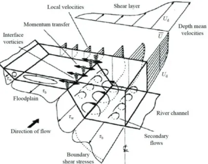
2.13 Schematic representation of natural river. Adapted from Filonovich (2015). . 48
2.15 Isovels of stream-wise velocity and secondary currents in rectangular open-channel for aspect ratio 2. Adapted from Tominaga et al. (1989) . . . 50
2.16 Calculated secondary current streamlines in open-channels under various as-pect ratios. Adapted from Naot and Rodi (1982). . . 50
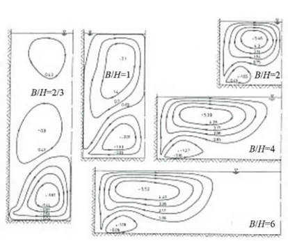
2.17 Predicted (RSM) and measured secondary flow in rectangular open-channel of differing aspect ratios (B/H). Adapted from Cokljat and Younis (1995). . . 51
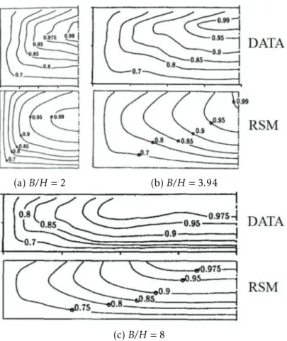
2.18 Contours of primary velocity for flow in rectangular open-channel of differing
aspect ratios (B/H). Adapted from Cokljat and Younis (1995). . . 52
2.19 Predicted (Reynolds Stress Model (RSM)) and measured turbulence anysotropy for open rectangular channel with aspect ratioB/H= 2. Adapted from Cokljat and Younis (1995). . . 52
2.20 Secondary current vectors in open-channel flow. Comparison between RSM (a and c) and LES (d) numerical studies and experimental study (2.20b). Adapted from Filonovich (2015). . . 53
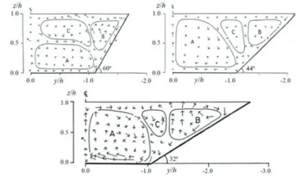
2.21 Secondary current vectors in smooth trapezoidal channels. Adapted from Tominaga et al. (1989). . . 54
2.22 Secondary flow cells pattern in smooth trapezoidal channels with different
aspect ratio 2bC/H. Adapted from Knight et al. (2007).. . . 54
2.23 Velocity contours and secondary velocity vectors in smooth trapezoidal chan-nels for different turbulence models. Adapted from Knight et al. (2005). . . 55
2.24 Schematic representation of different types of compound channel
configura-tion. Adapted from Filonovich (2015). . . 56
2.25 Hydraulic parameters associated with overbank flow in a trapezoidal com-pound channel. Adapted from Shiono and Knight (1991). . . 57
2.26 Schematic representation of flow field in varying rectangular compound chan-nel relative depth. Adapted from Nezu et al. (1999). . . 59
2.27 Experimental and computed stream-wise velocity contours. Adapted from Filonovich (2015). . . 60
2.28 Secondary current vector plots and primary velocity contour plots in asym-metric compound channels for hr = 0.5. Adapted from Cokljat and Younis
(1995). . . 60
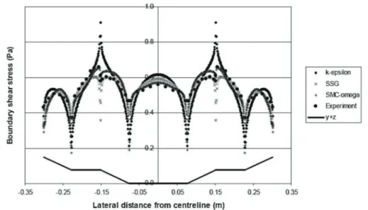
2.29 Boundary shear stress in symmetric compound channel with trapezoidal cross-section. Adapted from Knight et al. (2005). . . 62
3.1 Overview of OpenFOAM structure. Adapted from (CFD Direct, 2014).. . . . 66
3.2 Simplified overview of OpenFOAM distribution hierarchy. Adapted from Higuera Caubilla (2017). Used with permission.. . . 67
3.3 porousSimpleFoamcase structure. . . 69
3.4 A flow chart of the Semi-Implicit Method for Pressure Linked Equations (SIM-PLE) algorithm. Adapted from Moukalled et al. (2016). . . 71
3.6 porousSimpleFOAMsource code folder structure. . . 74
4.1 Adapted schematic description of floodplain open-channel flow from Tomi-naga and Nezu (1991). . . 81
4.2 Isovels of primary mean stream-wise velocity U for experimental case S-2. Adapted from Tominaga and Nezu (1991). . . 82
4.3 Secondary current vectors for experimental caseS-2. Adapted from Tominaga and Nezu (1991). . . 82
4.4 Isovels of mean streamwise velocity U normalized by Umax. Adapted from
Filonovich et al. (2014). . . 83
4.5 Isovels of primary mean stream-wise velocityU normalized byUmax for nu-merical study of Tominaga and Nezu (1991) in OpenFOAM. . . 84
4.6 Vector plot for numerical study of Tominaga and Nezu (1991) in OpenFOAM. 85
4.7 Secondary flow velocity plot (normalized for maximum stream-wise velocity
Umax) for numerical study of Tominaga and Nezu (1991) in OpenFOAM. . . 86
4.8 Turbulent kinetic energy (TKE) (k) plot for numerical study of Tominaga and Nezu (1991) in OpenFOAM. . . 87
4.9 Cross-section from the asymmetric trapezoidal compound channel. Adapted from Filonovich et al. (2010). . . 87
4.10 Mesh elements cross section distribution forporousSimpleFOAMfor experi-mental study by Filonovich et al. (2010). . . 88
4.11 Measured vertical profiles of time-averaged velocity in the floodplain, in the upper and lower interfaces. Adapted from Filonovich et al. (2010). . . 90
4.12 Measured vertical profiles of time-averaged as per Figure 4.11 for OpenFOAM numerical study with BSL-EARSM turbulence model. . . 90
4.13 Isovel lines obtained numerically in cross-section x = 7 m with turbulence model: a)k−ǫ; b) Menter’s Shear-Stress Transport turbulence model (SST); and c) Explicit Algebraic Reynolds Stress Model (EARSM). Adapted from Filonovich et al. (2010). . . 91
4.14 Isovel lines obtained numerically in cross-sectionx= 7mfor numerical study of Filonovich et al. (2010) in OpenFOAM. . . 92
4.15 Secondary flow vectors obtained numerically in cross-section x = 7 m with EARSM turbulence model. Adapted from Filonovich et al. (2010). . . 93
4.16 Secondary flow vectors obtained numerically for Filonovich et al. (2010) in cross-sectionx= 7mwith OpenFOAM and BSL-EARSM turbulence model. . 93
4.17 Secondary flow obtained numerically for Filonovich et al. (2010) in cross-sectionx= 7mwith OpenFOAM and BSL-EARSM turbulence model. . . 93
4.18 TKE results [m2/s2], obtained numerically in cross-sectionx= 7mwith three
different turbulence models. Adapted from Filonovich et al. (2010). . . 94
4.20 Experimental setup. Adapted from Nezu and Sanjou (2008). . . 96
4.21 Allocation patterns of vegetation elements. Adapted from Nezu and Sanjou (2008). . . 96
4.22 OpenFOAM mesh cross-section forNezu2008.; Lopez and Garcia (1997) . . 97
4.23 Residuals of numerical study using three different turbulence models in Open-FOAM for caseExp. 1of Lopez and Garcia (1997). . . 100
4.24 Residuals of numerical study using three different turbulence models in Open-FOAM for caseA-10of Nezu and Sanjou (2008).. . . 101
4.25 Experimental compound open-channel: (a) Photograph from upstream (zoom of artificial grass); (b) Illustration of cross-section. Adapted from Brito et al. (2016). . . 102
4.26 Scheme of the computational domain and boundary conditions for numerical study in Brito et al. (2016). . . 104
4.27 Cross-sectional view of the computational mesh for hr = 0.30 in Brito et al. (2016). . . 105
4.28 Time-averaged stream-wise velocity field forhr = 0.30. Adapted from Brito et al. (2016). . . 106
4.29 Normalised stream-wise isovel plot for numerical study of Brito et al. (2016) hr= 0.30 in OpenFOAM. . . 106
4.30 Vertical time averaged stream-wise velocity profile: (a)y/B= 0.40; (b)y/B= 0.60. Adapted from Brito et al. (2016). . . 107
4.31 Vertical time averaged stream-wise velocity profile for numerical study of Brito et al. (2016)hr= 0.30 in OpenFOAM. . . 107
4.32 Secondary currents forhr= 0.30: (a) experimental; (b) numerical. Adapted from Brito et al. (2016). . . 108
4.33 Normalized secondary flow plot for numerical study of Brito et al. (2016) hr= 0.30 in OpenFOAM. . . 108
A.1 Velocity profiles on submerged flexible canopy flow with and without monami (a) and profiles of normalized turbulent stress in and above flexible canopy for two flow conditions, based on the data by Ghisalberti and Nepf, 2006. Adapted from Nepf (2012b). . . 128
A.2 Deviation of experimental data from Forchheimer linear equation (Barree and Conway, 2004). . . 132
A.3 Porous media flow regions. Adapted from Marques (2015). . . 133
A.4 Porous media flow withRep= 86. Adapted from Marques (2015). . . 134
A.5 Porous media flow withRep= 225. Adapted from Marques (2015). . . 134
2.1 Parameters of various porous models in eq. 2.47 for Bed-2. Adapted from Li and Ma (2011) . . . 29
2.2 Parameters of various porous models in eq. 2.47 for Bed-5. Adapted from Li and Ma (2011) . . . 30
2.3 Values of the constants in thek−ǫ model for open channel flows. Adapted
from Filonovich (2015) . . . 41
2.4 Values of the constants in thek−ωmodel for open channel flows. Adapted from Filonovich (2015) . . . 41
4.1 Lopez and Garcia (1997) experimental parameters . . . 98
4.2 Lopez and Garcia (1997) rectangular flume vegetation and porosity parameters 98
4.3 Nezu and Sanjou (2008) experimental parameters for A-10, B-10 and C-10 experiments . . . 98
4.4 Nezu and Sanjou (2008) rectangular flume vegetation and porosity parameters 99
4.5 Submerged vegetation and porosity parameters for Brito et al. (2016)hr= 0.30 experimental study . . . 102
4.6 Summary of experimental conditions for Brito et al. (2016)hr= 0.30 . . . 103
3.1 Code for setting up the collocated SIMPLE loop as per Figure 3.4 in the
simpleFoam.Cfile. . . 72
3.2 Code for reading ofDandFcoefficients with global coordinate system in
DarcyForchheimer.Cfile. . . 74
3.3 UEqn.Hfile structure with implicit porosity treatment section omitted. . 75
3.4 pEqn.Hfile structure with explicit porosity treatment relaxation factors. . 76
1D One Dimensional
2D Two Dimensional
3D Three Dimensional
ASM Algebraic Stress Model
BSL Menter’s BaSeLinek−ωturbulence model
BSL-EARSM Baseline Explicit Algebraic Reynolds Stress Model
CAD Computer Aided Design
CFD Computational Fluid Dynamics
CFX ANSYS-CFX
COHM CoHerence Method
DEMI Departamento de Engenharia Mecânica e Industrial
DNS Direct Numerical Simulation
EARSM Explicit Algebraic Reynolds Stress Model
FCF Flood Channel Facility
FCT Faculdade de Ciências e Tecnologia
FD Finite Difference
FP Flood Plain
FVM Finite Volume Method
GNU GNU’s Not Unix
GUI Graphical User Interface
HFA Hot Film Anemometry
HWA Hot Wire Anemometry
LDA Laser Doppler Anemometry
LES Large Eddy Simulation
LRR Launder-Reece-Rodi pressure strain rate correlation model
LRR-QI Quasi-isotropic LRR
LRR-IP Isotropization of production model of the LRR
MC Main Channel
MIT Massachusetts Institute of Technology
MPI Message Passing Interface
MRF Multiple Reference Frame
OpenFOAM Open Field Open Access Manipulation
PIV Particle Image Velocimetry
RANS Reynolds-Averaged Navier-Stokes
RAS Reynolds-Averaged Simulation
RHS Right Hand Side
RSM Reynolds Stress Model
SERC Science and Engineering Research Council
SIMPLE Semi-Implicit Method for Pressure Linked Equations
SKM Shiono and Knight Method
SMC Second Moment Closure
SMC-ω Second Moment Closure - Omega Reynolds Stress Model
SSG Speziale-Sarkar-Gatski pressure strain rate correlation turbu-lence model
SST Menter’s Shear-Stress Transport turbulence model
STDEV STandard DEViation
STL STereoLithography file format
SWAK4FOAM SWiss Army Knife for FOAM
TKE Turbulent kinetic energy
UNL Universidade Nova de Lisboa
VARANS Volumetric-averaged Reynolds-averaged Navier-Stokes
VoF Volume of Fluid
WDCM Weighted Divided Channel Method
Symbol Description Units
a Frontal area per volume [m-1]
aI Linear resistance coefficient [s·m-1]
a′I Mathematical adjustment constant used in fully turbulent flow regime
[-]
a′′I Mathematical adjustment constant used in Darcy flow regime
[-]
A Channel cross-section area [m2]
Ap Surface area of the particle [m2]
Asp Surface area of an equivalent volume sphere [m2] Aim Interfacial area between the solid and the
fluid phase within a porous matrix
[m2]
b Blade thickness [m]
bC Main channel bottom width in asymmetric channels
[m]
bI Non-linear resistance coefficient [s2·m-2] b′I Nonlinear constant used in fully turbulent
flow regime
[-]
B Channel width [m]
Bf p Floodplain width [m]
Bmc Main channel width [m]
C Scalar volume fraction [-]
CF Non-linear Forchheimer coefficient for the volumetric average Darcy-Forchheimer ex-tended model
[-]
Cβ Porous media interface stress jump coefficient [-]
CA Viscous term constant [-]
CB Inertial term constant [-]
CD Canopy drag coefficient [-]
Cµ Empirical constant [-]
Symbol Description Units
Cǫ2 Empirical constant [-]
CE Ergun constant [-]
d Characteristic diameter/width of the canopy elements
[m]
deq Equivalent particle diameter [m]
dp Particle diameter [m]
dsd Sauter mean diameter [m]
dv Average diameter of cylinders analogous to the synthetic grass elements used in an ex-periment
[m]
dvs Actual diameter of a particle [m]
D Darcy/linear coefficientαinOpenFoam [m-2]
DV Spatially averaged drag [-]
e1 porosityPropertiesaxis-rotation vector [-] e2 porosityPropertiesaxis-rotation vector [-] e3 porosityPropertiesaxis-rotation vector [-]
fi Body forces [N]
F Forchheimer/Non-Darcy coefficient β in
OpenFoam
[m-1]
g Gravitational acceleration [m·s-2]
hb Main Channel height [m]
hMC Main Channel depth [m]
hf p Floodplain height [m]
hFP Floodplain height [m]
h Canopy height [m]
hr Relative depth [-]
hv Vertically uniform grass height [m]
H Flow depth [m]
k Turbulence kinetic energy [m2·s-2]
I Hydraulic gradient [m·Kg-1]
kS Nikuradse’s absolut roughness [m]
K Intrinsic permeability [m2]
Kapp Apparent permeability [m2]
Kf Hydraulic conductivity tensor [m·s-1]
L Characteristic length [m]
Lc Canopy drag length scale [m]
l Turbulence length-scale [m]
Symbol Description Units
p′ Pressure deviations [Pa]
Pk Turbulence kinetic energy production [m2·s-2]
Q Flow discharge [m3·s-1]
R Total drag per unit volume acting on the fluid by the action of the porous structure
[-]
Re Reynolds number [-]
Red Reynolds number for time and spatially aver-aged velocity
[-]
Rep Porous medium Reynolds number [-]
−ui′u′j Reynolds stress tensor [m2·s-2]
S Spacing between canopy elements [m]
Si Source term in Navier-Stokes equations [-]
SV Specific surface area [m2s]
Sv Specific inter-facial area [m2s]
s Clearance for the non-obstructed flow pas-sage
[m]
t Time [s]
T Temperature [K]
TF Solid matrix temperature [K]
TS Fluid phase temperature [K]
U Streamwise velocity [m·s-1]
us Seepage velocity vector [m·s-1]
u Longitudinal velocity [m·s-1]
ui Velocity component in theidirection,u,vor w
[m·s-1]
ui′ Velocity component fluctuations in the i di-rection
[m·s-1]
u′ Longitudinal velocity fluctuations [m·s-1]
u∗ Frictional velocity [m·s-1]
huii Intrinsic (fluid) average ofu [m·s-1]
UA Cross section bulk velocity [m·s-1]
Umax Maximum stream-wise velocity [m·s-1]
UMC MC bulk velocity [m·s-1]
UFP FP bulk velocity [m·s-1]
u Velocity vector comprised by the components u,vandw
[m·s-1]
Ui Mean velocity component in the idirection, U,V orW
Symbol Description Units
uD Darcy velocity [m·s-1]
v Lateral velocity [m·s-1]
v′ Lateral velocity fluctuations [m·s-1]
Vp Volume of a particle [m3]
vcf Cross flow (secondary flow) velocity [m·s-1]
w Vertical velocity [m·s-1]
w′ Vertical velocity fluctuations [m·s-1]
x Longitudinal Cartesian Coordinate [m]
y Lateral Cartesian coordinate [m]
y+ Dimensionless wall distance in the y direc-tion
[-]
z Vertical Cartesian coordinate [m]
z+ Dimensionless wall distance in thezdirection [-]
z0 Displacement height [m]
zm Roughness height [m]
G r e e k S y m b o l s
α Darcy/Linear coefficient [m-2]
αω k−ωturbulence model empirical constant [-]
β Forchheimer/Non-Darcy coefficient [m-1]
β∗ Model constant [-]
βω k−ωturbulence model empirical constant [m-1]
β′ k−ωturbulence model empirical constant [-]
δe Penetration length scale [-]
∆ Variation in a given scalar [-]
Symbol Description Units
ǫ Turbulent dissipation or Dissipation rate [m2·s-3]
η Kolmogorov length scale [-]
ηp Passability coefficient [m]
γ Experimentally determined additional mass [-]
κ Von Kármán constant [-]
λ Roughness density [-]
µ Fluid viscosity [Kg·s-1]
µe Effective viscosity [Kg·s-1]
ˆ
µ Viscosity ratio [Kg·s-1]
ν Fluid kinematic viscosity [m2·s-1]
νt Turbulence eddy viscosity [-]
ω Dissipation frequency or Specific dissipation rate
[s-1]
Ω1 Stream-wise vorticity [s-1]
φ Porosity [-]
ϕ Solid Volume Fraction [-]
ψ Sphericity/Shape factor [-]
ρ Fluid density [Kg·m-3]
σǫ k−ǫturbulence model empirical constant [-]
Symbol Description Units
σk Turbulent Schmidt number [-]
τ Characteristic length [-]
τa Apparent shear stress [N·m-2]
τt Reynolds number transition constant [-]
τzu Vertical shear stress [Pa]
C
h
a
p
t
e
1
I n t r o d u c t i o n
"Essentially, all models are wrong, but some are useful." (Box and Draper,1987)
1.1 Background and Motivation
Floods are one of the costliest natural disasters to which mankind is subject to. The study of anthropomorphic climate change and its effects make the study of flooding phenomena
with the aid ofComputational Fluid Dynamicstools ever more pertinent. "Floods have a major (defining) impact on floodplains and have significant socio-economic importance. The relatively flat, generally fertile, land with an adjacent water supply has attracted a large proportion of the world’s human population to dwell on floodplains at the mercy of the hazards of major flooding, landslides and mudflows" (Marriott,1999).
According to Terrier (2010) "flood disasters are responsible for approximately a third of the financial losses due to natural disasters throughout the world and account for more than half of the fatalities". He also cites a study on the trends of such disaster occurrences which demonstrate that these figures have been increasing significantly in recent years, making the point that this rise is partly to blame on the twentieth century engineering perspective of alleviating these phenomena by way of hard engineering solutions in the form of embankments, channel straightening or detention reservoirs. "However, such methods often failed to fulfil their objectives. Floodplains, which had been developed, continued to flood in spite of costly flood alleviation schemes", prompting advocacy of a more open approach to flood control focusing on theMain Channel (MC)-Flood Plain (FP)ensemble rather than solely theMC.
this policy is a sound understanding of the hydrodynamic processes that link a floodplain to its channel" (Terrier,2010).
Compound channel flow is a complex phenomenon where the interaction between the
MCandFPgenerates a complicated flow structure. "In practice, the modelling of such typically three-dimensional flows structures, for example for design purposes, usually has to be simplified" (Terrier,2010), not only in terms of its overall geometry but in terms of other properties which have a critical impact on flow properties.
The presence of vegetation on the floodplain, traditionally regarded by flood engineers as a problem which hinders flow capacity, riparian vegetation is now recognised as an integral part of the solution given its proven ecological role, thus the need to accurately numerically model its effect on the aforementioned flow structures.
The effect of submerged vegetation in both simple and compound-channel flow has
been the topic of investigation for quite some time, with numerous experimental studies providing valuable data for the development and refinement of numeric algorithms that are cost effective by being both fastidious and swift on a practical engineering time scale.
Figure 1.1: Cost of computing power equal to an iPad2. Adapted from The Hamilton Project (2011).
(2011) (Figure 1.1). This remarkable diverging trend has made computational power, previously unattainable but to the wealthiest of governments, now readily available to the regular end user, and more so to financially limited research institutions and businesses.
Mathematical models which had been contemplated more than a century ago became useful with computers that could now put them into practice, and the available process-ing power could be further optimised by deliberate simplifications to applied models. However, these simplifications need to be validated given their often limited contextual applicability, so as to ensure that the results they produce are not only mathematically sound, but truly informative in regards to real world phenomena.
Another development that has aided in the rapid development ofCFDsolutions has been the advent of theopen-sourcemovement which re-established the academic princi-ples of source code sharing initially present in software development, which grew out of favour as computer programs became more complex and were turned into a commodity. The establishment of theGNUProject(GNU’s Not Unix (GNU)being a recursive acronym), first announced on September 27, 1983 by Richard Stallman atMIT, planted the seed for theopen-sourcesoftware movement, which was essentially a splinter group from the free-softwaremovement established by Stallman (Stallman,2016). "Free" not as in "free of charge", but as in freedom to run the software study it, modify it and share it. As Stallman (2016) himself puts it, "in practice, open source stands for criteria a little looser than those of free software. As far as we know, all existing released free software source code would qualify as open source. Nearly all open source software is free software, but there are exceptions". Given the often commercial applications and customizations of theOpenFOAM(CFD Direct,2017) toolbox used and referred to in this thesis work, the open-sourcemoniker will hence be used. Much like the mathematical models previously mentioned, so too these tools need validation for them to be applicable to real world situations.
1.2 Objectives and Methodology
The main objective of this thesis is to evaluate the use of theopen-sourceCFD toolbox
OpenFOAMin the study of vegetated open-channel flow with a porous media analogue to the rigid submerged vegetation. The use of porous media as an analogue to vegetation patches is not new, although its use has been typically used to simulate the effect of forest
canopies on atmospheric boundary flow (Lemos,2006; Peralta et al.,2014). Flows of the type which are the focus of this study, in which "a macroscopic interface exists between a porous media and a clear fluid, the configuration so formed is called ahybrid medium" (Lemos,2006).
Typically, the effect of submerged vegetation on open-channel flow has been accounted
for by a drag coefficient which has to be calibrated on a case by case basis (Brito et al.,
et al.,2016; Uittenbogaard,2003), a method which can be heavily reliant on assumptions which affect the validity of the results if not backed up by experience in the field.
In this thesis we start out by evaluating the performance of the porousSimpleFOAM solver from the OpenFOAM toolbox in conjunction with an added turbulence model by Jeyapaul (2015) and Yogesh (2017) on a rectangular compound channel flow case by Filonovich (2015), then trying to partially replicate the numerical study by Brito et al. (2016) which made use of a commercial software solution, both for the good results that it was able to achieve and as a stress test due to the complexities inherent in trapezoidal compound open-channel flow, as detailed in Filonovich (2015), and summed up in2.5.3
as well as Brito et al. (2016).
Finally, further numerical simulations are conducted based on select parts of the ex-perimental work of Lopez and Garcia (1997) and Nezu and Sanjou (2008) on rectangular open-channel flow, and comparison not only with that experimental, but also numerical work.
As mentioned above, theopen-sourcetoolboxOpenFOAMwill be used, in particular the porousSimpleFOAM solver which, as the name implies, is aSIMPLEalgorithm based solver for single-phase, steady-state, incompressible fluid turbulent flows with explicit or implicit porosity treatment.
1.3 Thesis Outline
The present work is divided into five chapters and one appendix. Chapter 1 introduces the reader to the studied topic, giving a background that motivated this study, stating the main objectives and a brief description of the methodology used to accomplish them, and presenting the outline of the thesis.
In Chapter 2 a brief review of fundamental theoretical concepts required to under-stand the phenomena involved in submerged vegetated flow and how it’s typically mod-elled. Then there’s an introduction to flow in porous media, how porosity is modelled and how to apply existing models to submerged vegetation. A brief overview of turbulence modelling and introduction to the turbulence models used in this work is presented and an abridged description the main aspects on numerical modelling of rectangular and trapezoidal compound channel flows is presented. This later section aims to illustrate the turbulent field in compound channel flows and the different numerical approaches used
previously by other authors in their simulations.
Chapter 3 introduces theOpenFOAM CFDtoolbox, structure of theCFDpackage, and the algorithms and numerical techniques used in this study. This chapter also presents the importance of convergence and mesh independence study inCFDsimulations.
Chapter 4 first presents the experimental and numerical study used for validation and the experimental studies used for the numerical simulations of this work.
work.
C
h
a
p
t
e
2
T h e o r e t i c a l F r a m e w o r k
2.1 Introduction
The main focus of this thesis is the validation of theOpenFOAMtoolbox for the study of submerged vegetated flows with the use of a porous media analogue. In order to properly set-up the numerical case studies and then evaluate their results, it is necessary to comprehend the complexities of submerged vegetated flows, porous and hybrid media flow, turbulence modelling and vegetated open-channel flows, the latter by focusing first on cases non vegetated flow of various complexities, and then taking into account the effect of the introduction of submerged vegetation to these types of flow.
There have been numerous studies focused on the impact of submerged vegetation on simple and compound channel flows. These studies offer an abundance of experimental
and numerical results (from commercial codes) to which one can compare and adequately validate untested codes.
However, the use of a porous media analogue for dense submerged vegetation has not yet become a commonly adopted "tried and tested" approach, although the few studies that do make use of this technique show it to be a promising technique.
This Chapter is divided into the reviews of the following subjects which are relevant to the validating ofOpenFOAMfor the study of these types of flow:
• Section2.2presents a definition of submerged vegetated flow, how the vegetation is typically characterized, modelled and the impact that it has on the fluid flow.
• Section2.4introduces basic concepts in turbulence modelling with basic formula-tion of the prevalent two-equaformula-tion models and brief descripformula-tions of more robust models able to account for the flow structures in open channel flow which were used to conduct both the studies in the bibliography as well as in this work.
• Finally, Section2.5summarizes the flow characteristics of open channel flow, both simple and vegetated, and their respective numerical simulation research.
2.2 Basic concepts in submerged vegetated flow
The presence of submerged vegetation (i.e., rooted vegetation with a vertical extent less than the water depth) in floodplains is common in flood situations. In order to adequately model the effects of submerged vegetation on open compound and/or rectangular
chan-nel flow by means of a porous medium, its necessary to first understand both how to characterize the vegetation at hand, and how its experimental real flow is affected so as
to assess the validity of its numerical study.
Brito et al. (2016) rely on Nepf (2012b) and Nepf (2012a) description and characteri-sation of vegetation parameters to characterize the geometric scales used to build up the porous media analogue (see Section2.3). What follows is a description of the characteris-tics of vegetated flow, pertaining to the topic at hand, based on Nepf (2012b) and Nepf (2012a) (original sources omitted), and complemented by additional sources.
As mentioned in the Nepf (2012b), "the presence of vegetation alters the velocity field across several scales, ranging from individual branches and blades on a single plant to the community of plants, called the meadow or canopy".
Although there are many aspect pertaining to submerged canopy flow which are adapted from terrestrial canopy flow (Nepf,2012b), "unlike terrestrial canopies, aquatic canopies can occupy all or a large fraction of the flow depth such that the dynamic impact of the canopy is felt over the entire flow domain". (Nepf,2012b)’s review focused on the fully developed flow structure over and through long canopies, of which this study is only concerned with the submerged kind.
2.2.1 Geometric scales
The canopy geometry is defined by the scale of its individual elements, namely the in-dividual stems and blades and the number of these elements per bed area. The frontal area per canopy volumea(known as the leaf area index in terrestrial canopy literature)
is defined as follows:
a= d
∆S2 [m
-1] (2.1)
where d is a characteristic diameter or width of the canopy elements, and ∆S the
is the frontal area per bed area,λ, known as the roughness density (Nepf,2012b). For vertically uniform grass heighthv (i.e., vertically uniform a), andz= 0 at the bed:
λ= Z hv
z=0a dz=ahv [-] (2.2)
A value ofλ>≈0.23 is considered to be a dense vegetation layer (Nepf,2012a). Vegetation density can also be be described by the solid volume fraction,ϕ, occupied by the canopy elements (see Section2.3.3.2). If the individual elements approximate an individual cylinder such as reed stems, then:
ϕ≈ πad4v [-] (2.3)
If the morphology of the elements is strap like, such as sea grasses, then:
ϕ= db
∆S2 =ab [-] (2.4)
whered is the blade width andbthe blade thickness (Nepf,2012b).
"Aquatic canopies exhibit a wide range of geometry. marsh grasses are relatively sparse withd = 0.1 to 1cm, [ϕ] = 0.001 to 0.1, anda= 0.01 to 0.07cm−1(...). Mangroves are among the densest canopies, with [ϕ] as high as 0.45, mean trunk diameters of 4 to 9cm, andaup to 0.2cm−1(...). Seagrasses havea= 0.01 to 1cm−1and [ϕ] = 0.01 to 0.1 (...). Emergent plants tend to have rounded stems for higher stiffness, and submerged
grasses tend to have a blade geometry in which the width (0.3 to 1cm) is larger than the thickness (≈0.1cm), in which cased is the blade width" (Nepf,2012b).
2.2.2 Momentum Scales
According to Nepf (2012b), "within a canopy, flow is forced to move around each branch or blade so that the velocity field is spatially heterogeneous at the scale of these elements. A double-averaging method is used to remove the element-scale spatial heterogeneity, in addition to the more common temporal averaging (...). We let the coordinates x andz
be parallel and normal to the local mean bed slope, with z= 0 at the bed and positive away from the bed. The velocity vectoru= (u,v,w) corresponds to the coordinates (x,y,z), respectively, The instantaneous velocity and pressurepfields are first decomposed into a time averaged (overbar) and deviations from the time average (single prime). The time-averaged quantities are further decomposed into a spatial mean (angle bracket) and deviations from the spatial mean (double prime). The spatial averaging volume is thin in the vertical direction, to preserve vertical variation in the canopy density, and large enough in the horizontal plane to include several stems (>∆S).
Using the double-averaging method, the streamwise momentum equation becomes":
Dhui
Dt =gsinθ− 1 ρ
∂hpi ∂x −
∂ ∂zhu′w′i
| {z }
(i)
−∂z∂hu′′w′′i | {z }
(ii)
+ν∂
2hui
∂z2
| {z }
(iii)
"Hereρis the water density,νthe kinematic viscosity,θis the bed slope, andgis the gravitational acceleration [(see Figure2.1)]. Termiis the spatial average of the Reynolds stress. Termii, called the dispersive stress, is the momentum flux associated with spatial correlations in the time-averaged velocity field [which has been shown to be] less than 10% of the Reynolds stress (termi) for [λ>0.1]. Termiiiis the viscous stress associated with the spatial variation inhui[(see Section2.4for detailed description of these terms)]. The final term,DV, is the spatially averaged drag associated with the canopy elements, which is often represented by a quadratic drag law:
Figure 2.1: 2D vegetated canopy open-channel flows and coordinate system. Adapted from Nezu and Sanjou (2008).
DV =1 2
CDa
1−φhui|hui| [-] (2.6)
whereCD is the canopy drag coefficient. Because the drag acts on the fluid within the canopy, which occupies only (1−φ) of the total volume, the drag is divided by the factor (1−φ). The canopy drag length scale,Lc, is defined from the quadratic law, i.e., based on the dimensional reasoningDV =hui2/Lc (...). From Equation [2.6],
Lc=
2(1−φ)
CDa [m] (2.7)
This represents the length scale over which the mean and turbulent flow components adjust to canopy drag. Because most aquatic canopies have high porosity (φ <0.1), this scale is commonly approximated by (CDa)−1.
The drag coefficient,CD, is affected by the canopy density, a; the element Reynolds
number, Red =huid/ν [(see Sections2.3.3.5andA.3)]; and the morphology of the indi-vidual canopy elements. (...). The Darcy-Forchheimer equation [(see Section2.3.4.2)] has also been used to described drag in wetlands (...) and coral canopies (...). For flexible vegetation, the posture of the bed is affected by the flow speed, a phenomenon called
force has been represented by altering the exponent in the drag law, while holdinga, the frontal area, constant at the undisturbed (no flow) value,a0. (...) In practice, it is difficult to characterize the frontal areaafor real plants, which has led to contradictory results in the dependency of drag on velocity" (Nepf,2012b).
Equation2.5is also know as theVARANSequation (Higuera Caubilla,2015; Marques,
2015), which determines the average flow in a porous medium (such as a submerged canopy) without taking account the exact direction of the flow, as illustrated in Figure
2.2.
In Pedras and Lemos (2001), it is shown that for the macroscopic momentum equation the order of integration (time average and volume average) "is immaterial in regard to the final expression obtained. Also, theTKEresulting from application of the two averaging operators, following both orders of integration, are different". This work and it sources
(Gray and Lee,1977; Slattery,1967; Whitaker,1969; Whitaker,1999) should be consulted for a more in-depth understanding of the application of the volumetric operator. In regards to the time-averaging operator, which is used when turbulence effects are of
concern, see section2.4.
Figure 2.2: Representation of fundamental VARANSprinciple. Adapted from Higuera Caubilla (2015).
For an application of theVARANSequations to submerged vegetated patches in Open-FOAMconsult Chen et al. (2015), where models for the drag (or sink) term by Pedras and Lemos (2001) and Uittenbogaard (2003) are compared.
2.2.3 Submerged Canopies
"The velocity within a submerged canopy has a range of behavior depending on the relative depth of submergence, defined as the ratio of flow depth, H, to canopy height,
(bed slope). The relative importance of these driving forces varies with the depth of submergence (Nepf,2000):
turbulent stress pressure gradient ∼
H
h −1 [-] (2.8)
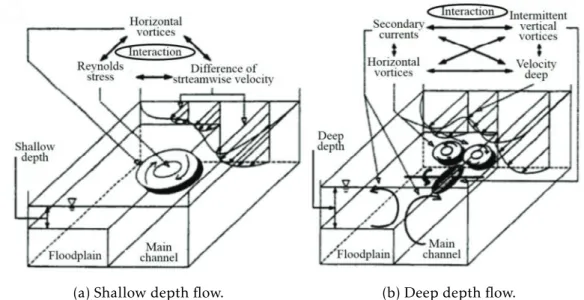
Three classes of canopy flow can be defined from Equation2.8: deeply submerged or unconfined (H/h>10), shallow submergence (H/h<5), and emergent (H/h= 1). A great
deal is known about unconfined canopy flow based on work in terrestrial canopies(...). When unconfined, the flow within a canopy is driven by the turbulent stress at the top of the canopy, i.e., by the vertical turbulent transport of momentum from the overflow, with negligible contribution from the pressure gradients. The terrestrial canopy model can be applied to aquatic canopies that are deeply submerged. However, because of the limitation of light penetration, most submerged aquatic canopies occur in the range of shallow submergenceH/h<5 (...), for which both turbulent stress and potential gradients are important in driving flow in the canopy. For emergent conditions (H/h= 1), flow is driven by the potential gradients, (...).
(a) Sparse canopy (λ≪0.1) (b) Transitional canopy (λ≈0.1) (c) Dense canopy (λ≫0.1)
Figure 2.3: Vertical (z) profile of longitudinal velocity and dominant turbulent scale for a sparse (a), transitional (b) and dense (c) canopies, where his the submerged canopy height andδe is the vortice fixed penetration length into the canopy. Adapted from Nepf (2012b).
For a submerged canopy, there are two limits of behaviour, depending on the relative importance of the bed drag and the canopy drag. If the canopy drag is small compared with the bed drag, then the velocity follows a turbulent boundary profile, with the veg-etation contributing to the bed roughness (sparse canopy; Figure 2.3a). If the canopy drag is large compared to the bed drag, the discontinuity in drag that occurs at the top of the canopy (z=h) generates a region of shear resembling a free shear layer with an inflection point near the top of the canopy (dense canopy, Figure2.3b,c)" (Nepf,2012b). Nepf (2012b) also states, based on his sources, that the transition between the sparse and dense regimes occurs at the roughness densityCDλ=ah= 0.1,CD being the canopy drag coefficient, with one study showing it be as high asCDλ= 0.15. "On the basis of measured
no inflection point ifCDah<0.04. A pronounced inflection point appears at the top of the canopy forCDah>0.1. BecauseCD ≈1 in most of the studies considered, these limits are consistent with the scaling and numerical estimates given above" (Nepf,2012b). He does stress that his review focuses only on unidirectional flow, and that in flow conditions dominated by waves the canopy drag may have little impact on induced wave velocity, a topic which he further elaborates on in his paper.
Focusing on the dense canopy conditions (λ>0.1) there is a demonstrated similarity between canopy sheer layers and free shear layers. "In a free shear layer, the velocity profile contains an inflection point, which triggers a flow instability that in turn leads to the generation of Kelvin-Helmholtz vortices (...). These structures dominate the transfer of momentum between the high speed and low-speed streams, and their size sets the length scale of the shear layer. For dense submerged canopies (λ>0.1), the momentum absorption by the canopy is sufficient to produce an inflection point in the velocity profile,
which, as in free shear layers, leads to the generation of Kelvin-Hulmholtz vortices (Figure
2.3b,c). These vortices are called canopy-scale turbulence to distinguish it from the much larger boundary-layer turbulence, which may form above a deeply submerged or unconfined canopy, and the much smaller stem-scale turbulence.
Over a deeply submerged (or terrestrial) canopy (H/h >10), the canopy scale vor-tices are highly three dimensional owing to their interaction with larger boundary-layer turbulence, which stretches the canopy-scale vortices, enhancing secondary instabilities (...). However, with shallow submergence (H/h≤5), which is common in aquatic sys-tems, larger-scale boundary-layer turbulence is not present, and the canopy-scale vortices dominate the turbulence field, both within and above the canopy (...). For shallow sub-mergence, the canopy scale turbulence is also more coherent (less than three dimensional) than that observed with deeply submerged (or terrestrial) conditions. However, in both cases, the canopy style vortices dominate the vertical transport at the canopy interface (...).
In a free shear layer, the vortices grow continually downstream, predominantly through vortex pairing (...). In canopy shear layers, however, the vortices reach a fixed scale and a fixed penetration into the canopy (δe in Figure 2.3b,c) at a short distance from the canopy’s leading edge (...). On the basis of measurments with a flexible model of the sea-grassZ. marina(a= 5.7m−1), a fixed shear layer scale is reached at a distance of 10hfrom the leading edge of the meadow (...). The fixed vortex and shear-layer scale is reached when the shear production that feeds energy into the canopy-scale vortices is balanced by dissipation by canopy drag. This energy balance predicts the following length scale, which has been verified by laboratory observations (...)" (Nepf,2012b):
δe=0.23±0.6 CDa
[-] (2.9)
whereCD is the Canopy drag coefficient. As mentioned previously a factor ofCDλ≥
canopies. "In the range CDλ= [0.1,0.23], the shear layer vortices penetrate to the bed,
δe=h, creating a highly turbulent condition over the entire canopy height (Figure [2.3b]). At higher values ofCDλ, the canopy scale vortices do not penetrate to the bed, δe <h
(Figure2.3c).
The scalingδe∼a−1has been observed in flows near porous layers over a wide range of physical scales, from granular beds to terrestrial forests and urban canopies (...). However, the scale relation must brake down when (CDa)−1 approaches the scale of the canopy elements ,d, becauseais defined only as an average over multiple elements. For rigid cylinders, when (CDa)−1 is less than 2d, the penetration scale transitions to a constant
δe≈2d (...). The depth of submergence,H/h, can also affect the penetration length scale.
ForH/h<2,δeis diminished from Equation [2.9], as interaction with the water surface diminishes the scale and the strength of the vortices.
The penetration length,δe, segregates the canopy into an upper layer of strong tur-bulence and rapid renewal and a lower layer of weak turtur-bulence and slow renewal (...). Flushing of the upper canopy is enhanced by the canopy-scale vortices that penetrate this region (Figure [2.3c]). In contrast, turbulence in the lower canopy (z<h−δe) is generated in stem wakes and has a significantly smaller scale, set by the stem diameters and spacing. Canopies for whichδe/h<1 (Figure [2.3c]) shield the bed from strong turbulence and turbulent stress. Because turbulence near the bed plays a role in resuspension, these dense canopies are expected to reduce resuspension and trap sediment. (...). We note that the transition in near-bed turbulence and resuspension does not occur abruptly at
CDλ = 0.23 but occurs gradually with increasingCDλ above this value, as the canopy scale vortices are progressively pushed further from the bed. Because of the reduced near-bed turbulence, dense canopies can promote sediment retention. In sandy regions, which tend to be nutrient poor, the preferential retention of fines and organic material (i.e., muddification) enhances the supply of nutrients to the canopy so that dense canopies provide a positive feedback to canopy health in sandy regions. In contrast, in regions with muddy substrate, which is more susceptible to anoxia [(lack of oxygen)], sparse meadows (CDλ≤0.23) may be more successful because the enhanced near-bed turbulence removes fines, leading to a sandier substrate that is less prone to anoxia" (Nepf,2012b).
"In compound open-channel flowsH/h(see Figure2.4a) is a function of the relative depthhr, defined as the relation betweenFP flow depthhFP andMCflow depthhMC" (Brito et al.,2016):
hr=hhFP MC
[-] (2.10)
2.2.4 Mean Velocity Profile
Based on Nepf (2012b)’s description of vegetated flow so far, "sufficiently far above a
(a) Compound open-channel withMain Channel andFlood Plain.
(b) Rectangular open-channel flow.
Figure 2.4: Cross-sections of open-channel flow geometries with vegetation. Adapted from Fischer-Antze et al. (2001).
hui=u∗
κ ln z−zm
z0 !
[m·s-1] (2.11)
withκ= 0.4 (von Kármán constant). The horizontal average (in angled brackets) is not strictly needed above the canopy but is retained for consistency with the equations within the canopy. The friction velocity,u∗, is related to the Reynolds stress at the top of the canopy,u∗2=hu′w′ih. The parameterszmandz0are the displacement and roughness
heights, respectively, both of which depend on the canopy roughness density, λ. On the basis of studies with both model and real vegetation, a simple estimate for friction velocity is":
u∗= [gS(H−h)]0.5 [m·s-1] (2.12)
withSdefined as:
S=∂H
∂x + sinθ [m] (2.13)
"If the vegetation is flexible, thenhis the mean deflected height of the canopy (...).
However, if the depth of submergence is small, compared to the displacement height, the following estimator is more accurate":
The "penetration length scale, δe [(Figure 2.3)], describes the distance over which turbulent stress penetrates the canopy from above. Similarly, the displacement height is the centroid of momentum penetration into the canopy (...). This similarly suggests the physically intuitive scaling":
zm h ≈1−
1 2
δe h = 1−
0.1 CDλ
[-] (2.15)
"which has been confirmed forλ≈[0.2,0.3] (...). Forλ>1, the displacement thickness tends towards zm ≈h, indicating that essentially the entire canopy is cut off from the overflow. In addition,zmgoes to zero atλ= 0.1. Whenzm= 0, the velocity profile has no inflection point (Figure [2.3a), consistent with the observation thatλ>0.1 is required to produce an inflection point in measured velocity profiles (Figure [2.3b,c]).
The dependency of the roughness height,z0, on the canopy density,λ, differs signifi-cantly above and below the threshold ofλ= 0.1 (...). In the sparse-canopy range (λ<0.1), the roughness height increases with increasingλ. In sparse canopies, the flow penetrates
the full canopy so thatz0is proportional to the drag imparted by the full canopy,CDλ, i.e.,
z0/h∼CDλ. In contrast, for dense canopies (λ>0.1), the roughness height decreases with increasing λ. The effective heigh of the canopy, as seen by the overflow, is the
penetra-tion scale,δe. The roughness height depends on this effective height, rather than canopy
height, so thatz0∼δe∼a−1. (...).
The logarithmic profile form is based on equilibrium turbulence such that dissipation and production are locally in balance (...). Largely because of the vertical transport provided by the shear layer structures, this condition is not met for some distance above the canopy, called the roughness sublayer. For very shallow submergence,H/h≤1.5, the roughness sublayer extends to the surface, and a logarithmic structure is not observed above the canopy".
Nepf (2012b) goes on to describe the velocity profile within the bed so as to obtain a reasonably accurate full velocity profile by combining the models for above-canopy and in-canopy profiles. This is illustrated in Figure2.5which contains the measured velocity (dots) and predicted velocity (solid line) with confidence line (dashed lines) from Ghisal-berti,2005. Parameters are: H= 46.7cm,h= 13.9cm,S= 2.5×10⁻⁵,a= 0.034cm−1, and CD= 0.77 (measured). Above the meadow, the velocity is predicted from the logarithmic profile (Equation2.11), with friction velocity as per Equation2.12, zmas per Equation
2.15, andz0= (0.04±0.02)a−1. For the equations used to determine the in-canopy velocity profile please consult the source.
Given that the use of a porous medium as an analogue to a dense submerged canopy nullifies any study of a valid in-canopy velocity profile (Marques,2015; Sonnenwald et al.,
Figure 2.5: Measured velocity (dots) and predicted velocity (solid line) with confidence line (dashed lines) from Ghisalberti,2005. Adapted from Nepf (2012b).
2.3 Basic concepts in porous media flow
A porous medium can be described as a solid (or solid matrix) with interconnected voids distributed somewhat uniformly throughout the bulk of the body (Jambhekar, 2011; Polezhaev,2006), of which its main characteristic isporosity,φ(Equation2.17).
The use of porous media in CFD goes beyond its initial applicability in describing actual physical porous structures. It extends to other physical structures, which on a physical level, act as a porous medium in the way that these structures might dampen the flow of a given fluid, and even redirect its flow, such as the use of porous media as an analogue for swirl vanes in a gas turbine engine as in Ford et al. (2013).
It is therefore a topic of great interest in various scientific and technical fields, with wide applications in the field of engineering (Jambhekar,2011; Li and Ma,2011; Nield and Bejan,2013) as can be seen in Figure2.6.
(a) Catalytic converter for automobile exhaust sys-tem
(b) Porous heat exchanger for air cooled condensers
(c) Cooling pores in a gas turbine blade
As stated in chapter1, this thesis has as its main purpose the validation of the use of a porous medium as a stand-in for a submerged dense vegetative layer, as initially validated by Brito et al. (2016) and more recently Sonnenwald et al. (2016), using theOpenFOAM
open-source tool. Although limited (Marques,2015; Sonnenwald et al.,2016), the use of a porous medium to simulate a vegetative layer provides a more pragmatic and scientific approach to achieving valid numeric simulations of the effects of submerged vegetation
(Brito et al.,2016; Sonnenwald et al.,2016), effects which have been traditionally taken
into account by introducing an extra sink term into the momentum equations, thus accounting for the additional flow resistance of the submerged vegetation. This term is usually "modelled as a drag force on a rigid obstacle (cylinder/vegetation element) with drag coefficient of an isolated cylinder, accounting for both viscous and form drag
arising from the spatial perturbation of velocity and pressure" (Brito et al.,2016). There are similar methods which use more complex turbulence models such as RSM, which are more computationally expensive to run (Cebeci,2004; Filonovich,2015; Pope,2000; Versteeg and Malalasekera, 2007), or which just make use of a bulk drag coefficient.
However, these approaches have their own limitations. The method which makes use of a cylinder’s drag coefficient, though able to reproduce the flow velocity profiles, disregards
eddy-eddy and eddy-cylinder interactions, as well as being unable to properly address the vegetation spatial heterogeneity and requiring a numerical mesh fine enough to account for individual vegetation elements (Brito et al.,2016).
In his Master’s thesis, Jambhekar (2011) thoroughly describes the fundamentals of Darcy and non-Darcy (Forchheimer) flow models. What follows is a literature review composed of mainly this source complemented by additional sources. However, some details will be abridged or omitted due to the particular nature of the type of porous media flow which is the scope of this thesis, namely isothermal single-phase steady-state flow in porous media.
2.3.1 Scales - The continuum approach
How one treats the problem of flow through a porous medium is largely dependent on the scale considered. It is only convenient to apply a conventional fluid mechanics approach to the flow phenomenon in the fluid filled spaces if one is looking at a micro-scale or pore-scale, analysing the flow in a particular section of the porous medium. In cases such as those being studied in this thesis, i.e. the macro-scale, such an approach is not feasible due to the complicated flow paths and the need to describe the complex spatial resolution of the porous structure, requiring an excessively refined mesh in order to accurately describe the flow (Jambhekar,2011).
continuum at the macro-scale is a fundamental concept of fluid mechanics" (Jambhekar,
2011).
In Brito et al. (2016), Lemos (2006), and Pedras and Lemos (2001), the continuum approach is adopted by means of a volume averaged approach so as to describe the flow properties on a macro-scale. Figure 2.7 illustrates the different scales involved in the
averaging process.
Figure 2.7: Micro-scale to macro-scale transition. Adapted from Jambhekar (2011).
The domain is first analysed at the micro-scale (see Section2.3.3) and its properties are averaged over aRepresentative Elementary Volume (REV)"in order to obtain a macro-scale description of the system with effective parameters such as porosity φ (...) and
intrinsic permeabilityK" (see Section2.3.4). "The macro scale is also referred to as the
REV-scale. It can be seen from Figure"2.7"that at the REVscale, detailed spatial reso-lution of solid matrix and fluid phase is lost, and effective volume averaged parameters
(effective parameters) are available" (Jambhekar,2011).
The volume averaged quantities need to be independent from theREV-size, so the latter must be properly selected. This is illustrated in Figure2.8, where it’s shown that the selectedREVshould be smaller than the flow domain and larger than a single pore in the porous medium. This is to avoid both oscillations due to existence of inhomogenieties at the micro-scale, and fluctuations caused by macroscopic heterogeneities of the medium (Jambhekar,2011).
2.3.2 Local equilibrium in porous media
"The local thermodynamic equilibrium in porous media mainly consists of thermal, chem-ical and mechanchem-ical equilibria as follows: