Drone Route Optimization using Constrained Based Local Search

Sérgio Bairos Pimentel

Drone Route Optimization using Constrained

Based Local Search

Dissertação para obtenção do Grau de Mestre em

Engenharia Informática

Orientador: Prof. Doutor Pedro Barahona, Professor Catedrático, Universidade Nova de Lisboa

Co-orientador: Prof. Doutor Carlos Damásio, Professor Associado, Universidade Nova de Lisboa

Júri

Presidente: Prof. Doutor José Júlio Alves Alferes

Vogais: Profª. Doutora Paula Alexandra da Costa Amaral Prof. Doutor Pedro Barahona

Drone Route Optimization using Constrained Based Local Search

Copyright © Sérgio Bairos Pimentel, Faculdade de Ciências e Tecnologia, Universidade NOVA de Lisboa.

A Faculdade de Ciências e Tecnologia e a Universidade NOVA de Lisboa têm o direito, perpétuo e sem limites geográficos, de arquivar e publicar esta dissertação através de exemplares impressos reproduzidos em papel ou de forma digital, ou por qualquer outro meio conhecido ou que venha a ser inventado, e de a divulgar através de repositórios científicos e de admitir a sua cópia e distribuição com objetivos educacionais ou de inves-tigação, não comerciais, desde que seja dado crédito ao autor e editor.

Este documento foi gerado utilizando o processador (pdf)LA_{TEX, com base no template “novathesis” [1] desenvolvido no Dep. Informática da FCT-NOVA [2].}

A c k n o w l e d g e m e n t s

This academic journey has been one of the most rewarding experiences of my life and i am grateful that it occurred on one of the most prestigious colleges in the country. I have found to be true all the good things that were mentioned by so many people about the faculty, whether if it was about the academic environment, the helpful colleagues, the teachers, or the constant vivid activity on the campus. Needless to say, there were some ups and downs, as it normally goes. As such, i would like to thank Universidade Nova de Lisboa - Faculdade de Ciências e Tecnologias for allowing me to grow so much professionally and emotionally as i did the past years. I would also like to thank my adviser, Prof. Pedro Barahona, for guiding me through the elaboration of this thesis and whose help was essential, and my co-adviser Prof. Carlos Damásio for having this interesting thesis subject. To all my class mates that i have encountered throughout the years and that made this adventure much easier and funnier. To my beautiful girlfriend Natacha Teves. Your peacefulness has definitely helped throughout these academic years and i hope i can help you go through yours too. Finally, to my family. To my mother for pushing me to be more disciplined and organized, to my sister for showing me how to be dedicated, to my brother in law for showing me how to be well informed, to my nephew for bringing even more joy to our family, and to my father for showing me how to be ingenious and consistent. Thank you all for giving me so much, and i really hope i can give you so much more in days to come.

A b s t r a c t

This dissertation focuses on an optimization problem that consists of finding the best flight plan (i.e. routes) for an Unmanned Aerial Vehicle (UAV), or drone, overflying a farming field that needs to be swept and sprayed with fertilizers or pesticides. This system calculates an optimal route for a crop field, having into consideration that the field needs to be swept and covered entirely. Drones have been around for many years, especially in the military, but only recently they have expanded to other fields, including agriculture, which makes it a particularly interesting field of study. The drones we consider in this thesis are not any regular type of drone for common use, but rather a specially adapted drone for agriculture to facilitate the process of farming. These drones fly close to the ground spraying fertilizers using specialized extension tools. Therefore, the main prob-lem is to search for an efficient route that sweeps the field and saves as much resources as

possible. Additionally, the resolution to this problem should not only consist of searching for an ideal route, but also to help the user in planning and selecting a desired field. Some factors need to be taken into account when considering such problems such as legislation, drone’s energy consumption, and environment related variables such as field elevations or man-made infrastructures. This system is built using local search as a basis, which essentially consists in making small changes to a solution, improving it iteratively until some near optimal solution is hopefully found.

Keywords: Drone, Local Search, Farming, Optimization, Route, Coverage Path Planning Problem.

R e s u m o

O tema desta tese foca-se num problema de otimização que consiste em encontrar o me-lhor plano de voo (i.e. rotas) para um veículo aéreo não tripulado (UAV ou drone em inglês), a sobrevoar um campo de cultivo, que necessita de ser pulverizado com produtos químicos tais como fertilizantes ou pesticidas. Este sistema pretende calcular uma rota ótima para qualquer campo de cultivo, tendo em conta que este campo precisa de ser coberto inteiramente. Os drones já marcaram a sua presença há muitos anos atrás na área militar, mas apenas recentemente é que tiveram uma forte expansão para muitas outras áreas, uma delas sendo a agricultura, o que torna o estudo desta tese particularmente interessante. Estes drones são especialmente adaptados para agricultura e facilitam o processo de cultivo. Sobrevoam os campos a uma altitude relativamente baixa e pulveri-zam químicos usando extensões mecanizadas incorporadas no próprio drone. O problema principal é, portanto, procurar uma rota eficiente que otimize o número de recursos dispo-nível. Adicionalmente, a resolução para este problema deve não só consistir em procurar a rota ideal, como também fornecer ao utilizador a ajuda necessária para planear e sele-cionar um campo de cultivo à sua escolha. É necessário ter em conta alguns fatores para este problema tais como legislação, modelo específico do drone em termos de consumo de energia e variáveis ambientais, como por exemplo relevos nos campos ou infraestruturas. O sistema baseia-se na técnica de pesquisa local que consiste em efetuar alterações a uma solução até que eventualmente tenhamos uma solução (quase) ótima.

Palavras-chave: Veículo Aéreo não Tripulado, Pesquisa Local, Agricultura, Otimização, Rotas, Coverage Path Planning Problem.

C o n t e n t s

List of Figures xv

List of Tables xix

Listings xxi

Glossary xxiii

Acronyms xxv

1 Introduction 1

1.1 Motivation . . . 1

1.2 Objectives . . . 1

1.3 Contributions . . . 2

1.4 Thesis Overview . . . 2

2 Context 3 2.1 SkyScan . . . 3

2.2 Legislation . . . 3

2.3 The Route Optimization problem . . . 4

3 Related Work 7 3.1 Coverage Path Planner . . . 7

3.2 Local Search Metaheuristics . . . 10

3.2.1 Tabu Search . . . 10

3.2.2 Variable Neighborhood Search. . . 10

3.2.3 Simulated Annealing . . . 11

4 System Architecture 13 4.1 Main Components . . . 13

4.2 Interface . . . 14

4.2.1 Interface pre-processing and other features . . . 16

4.3 Planner Debugger/Visualizer . . . 17

4.4 Tools . . . 18

C O N T E N T S

5 Coverage Path Planner 21

5.1 Description . . . 21

5.2 Problem Modeling. . . 21

5.3 Implementation . . . 23

5.4 Scaling the planner . . . 30

6 Results 31 6.1 Tests Structure . . . 31

6.2 Metaheuristic test with no weights . . . 32

6.3 Weighted Metaheuristic test . . . 34

6.4 Benchmark test . . . 36

6.4.1 Consistency test . . . 39

6.5 Case scenarios . . . 41

6.5.1 Simple scenario . . . 41

6.5.2 Elevated scenario . . . 42

6.5.3 Obstacle scenario . . . 45

7 Conclusion 49 7.0.1 Future work . . . 50

Bibliography 53

L i s t o f F i g u r e s

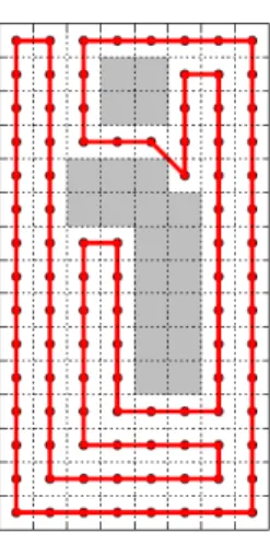
2.1 An environment scenario. The image illustrates a crop with some obstacles represented as red cells. The yellow cells are the start and end cells in which the drone will initialize and end its flight. The brown cells is the field that the operator wishes to fertilize.. . . 5

2.2 Close up of an area. Each area is represented as a grid with cells. It is assumed that the drone covers each cell entirely when it passes through it. . . 5

2.3 Example of a path taken by a drone considering two coordinates and angle of turns. . . 5

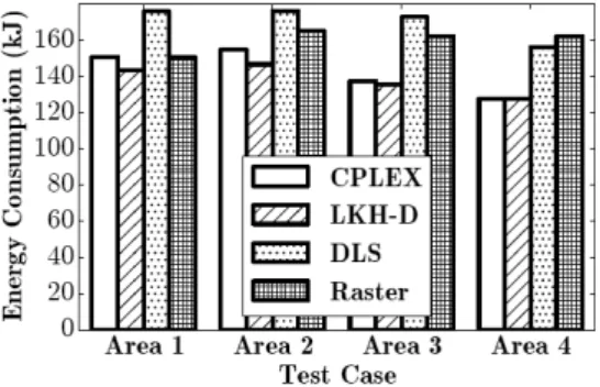
3.1 Energy consumption on each of the four different type of areas, using four algorithms. Their algorithm is the Lin-Kerninghan Heuristic for Drones (LKH-D) which was successful in comparison to the other three. . . 8

3.2 The two types of sweeps in a rectangular field. . . 8

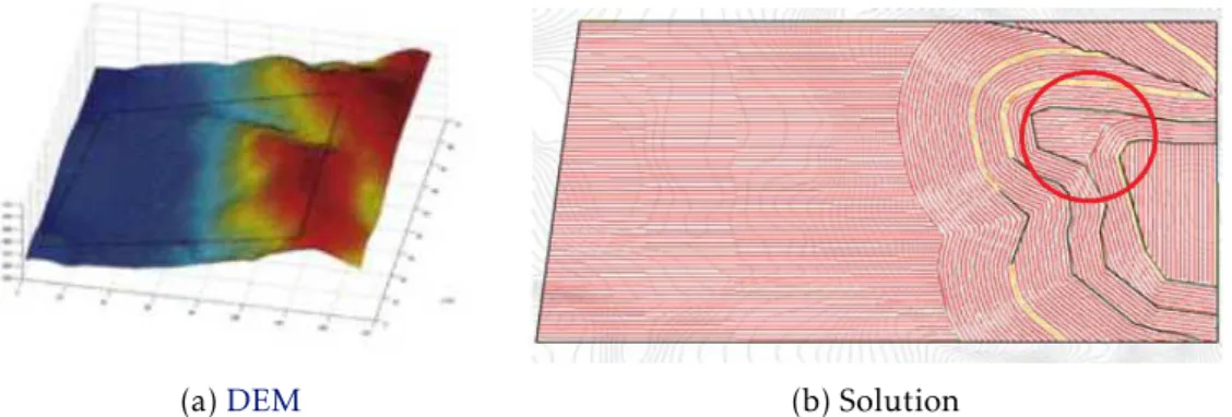
3.3 The digital elevation map (a) and the corresponding solution (b). . . 9

4.1 System Architecture. The user creates real life instances with the interface which is then provided to the planner. . . 13

4.2 The entire application. The map displays the flight restrictions all over Portu-gal provided by Autoridade Nacional da Aviação Civil (ANAC) and a tool bar to aid the field selection and generation. Field Restrictions can be toggled on or offin the top center of the display. . . 14 4.3 Flight restrictions in Portugal. By clicking in a restricted area, the

correspond-ing description is displayed with important information for the drone operator. 15

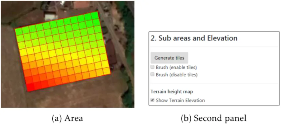
4.4 Demonstration of the area (b) being fit onto the desired field (a) using the first panel of the interface (c) to scale and rotate. . . 15

4.5 Demonstration of the tiles being generated and selection of obstacles (a) using the second panel of the interface (b). Red cells are obstacles and green cells are flyable cells. . . 16

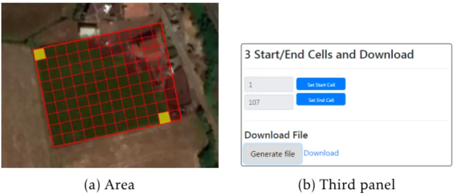
4.6 Selection of the start and end cell (a) using the third panel (b). . . 16

4.7 Elevation of the terrain. Shades of red represent higher elevations while shades of green represent lower elevations. . . 17

L i s t o f F i g u r e s

4.8 The same field instance at different moments in time. The progress occurs from top to bottom, left to right, with decreasing cost at each step. The route is initialized randomly in the first moment of the progress. Cells 7 and 8 are obstacles and are not covered. Cells 1 and 4 is the start and finish position respectively. . . 18

5.1 Example of an area to be swept represented as a oriented graph. The black node is an obstacle. The graph is oriented since the difference in altitudes are considered. . . 22

5.2 A cell and its neighbors, and the exterior angle for three nodes on the path . 23

5.3 The field (a) and the elevations of each cell (b). The start cell is 1 and the finish cell is 4. . . 24

5.4 A very small example of an area to be swept with one obstacle (cell 6). . . 25

5.5 A non optimal solution. The path taken from cell 1 to 3 is through cell 2. From 3 to 5 is direct since they are adjacent. . . 28

5.6 The field instance from the paper chosen as a benchmark [9] with obstacles as grey cells. On the left the normal field and at the right all the 8 sub-areas generated delimited as diff_{erent shades of green. . . . . 30}

6.1 The basic field. This field is 10x10 units long and has no obstacles. The elevation was obtained with the interface by dragging the 10x10 area onto a random location. The start and ending point is the top left cell. . . 33

6.2 The results for the metaheuristic test. The vertical axis represents the mini-mum cost of all tries with the respective configuration and the the horizontal axis (top) the meta heuristic used with corresponding parameter values. The bottom horizontal axis is the initial route. . . 34

6.3 The impact of the angle (blue) and distance (orange) costs in the overall cost for diff_{erent values ofka. . . . . 37} 6.4 The average number of turns (in degrees) of a solution for different values of

ka. . . 38

6.5 The best solutions for the benchmark test. . . 39

6.6 The best and worst solutions obtained from the consistency test. . . 40

6.7 The simple scenario. The field is 9x12 units long. In (c), the start point is the top left yellow point and the finish is the bottom right point. . . 41

6.8 The initial route (a) using field sweep, and the solution (b). . . 41

6.9 The second scenario. The starting point is at the top left corner and the finish point in the bottom right.. . . 42

6.10 The elevation of the second scenario. . . 43

6.11 The penalty of elevation (yellow) added to the cost of distances (blue) for different penalty weights.. . . 43 6.12 The average number of climbs (meters) for different values of_kh . . . 44

L i s t o f F i g u r e s

6.13 Two distinct solutions for the second scenario. . . 45

6.14 The third scenario. The starting point is the cell from the top and the finish point the one from the bottom. . . 46

6.15 The elevation of the third scenario. . . 46

6.16 Three distinct solutions for the third scenario. . . 46

L i s t o f Ta b l e s

5.1 The adjacency cost matrix. . . 25

5.2 The updated cost matrix. . . 27

6.1 The weighted metaheuristic test with different altitude and angle weights. For each combination, the minimum cost is displayed from a series of tries. . . . 35

6.2 Heuristic comparison. . . 35

6.3 The configuration of parameters that were set when the different solutions were obtained. The last three columns stand for distance cost, angle cost, and the sum of turns taken (in degrees), respectively. . . 39

6.4 Initial route comparison for the benchmark test. . . 39

6.5 The results obtained from all the tries (10) where each try has a maximum runtime of 5 minutes. The last three columns stand for distance cost, angle cost, and the sum of turns taken (in degrees), respectively. The variation column tells us how diff_{erent the solutions are when compared to the best in} terms of overall cost. . . 40

6.6 Initial route comparison for the simple scenario. . . 42

6.7 The configuration of parameters that were set when the different solutions were obtained. The last five columns stand for distance cost (dc), eleva-tion/height cost (hc), angle cost (ac), the sum of turns taken (in degrees) (tt), and climb sum (cs), respectively. . . 45

6.8 The configuration of parameters that were set when the different solutions were obtained. The last five columns stand for distance cost (dc), eleva-tion/height cost (hc), angle cost (ac), the sum of turns taken (in degrees) (tt), and climb sum (cs), respectively.. . . 47

L i s t i n g s

5.1 File structure . . . 24

5.2 Floyd-Warshall’s algorithm . . . 26

5.3 Floyd-Warshall’s algorithm updated. . . 26

5.4 Path reconstruction . . . 27

G l o s s a r y

CPLEX An optimization software package developed by IBM.

Hyperspectral Hyperspectral sensors are devices capable of gathering data using the reflective spectrum of an object. Regular cameras use the visible spec-trum for imagery, while hyperspectral cameras gather information from most of the spectrum (visible and not visible), which helps identify im-portant characteristics in the target object.

Instance In this thesis context, an instance is a data structure that represents the field to be swept and has information about the obstacles, initial/fin-ishing cell and the elevations of each cell.

Load Balance The load balance algorithm consists in improving the distribution of workloads across multiple resource consumers.

Local Search The process of iteratively modifying some solution in order to improve it, by doing small changes to that solution.

Metaheuristic A procedure that helps local search to escape from local optima.

A c r o n y m s

ANAC Autoridade Nacional da Aviação Civil.

CPP Coverage Path Planning Problem.

DEM Digital Elevation Map.

ITS-TSP Intelligent Transportation Systems Traveling Salesman Problem.

LKH-D Lin-Kerninghan Heuristic for Drones.

NIR Near-Infrared.

SA Simulated Annealing.

TSP Traveling Salesman Problem.

UAV Unmanned Aerial Vehicle.

VNS Variable Neighborhood Search.

C

h

a

p

t

e

r

1

I n t r o d u c t i o n

1.1 Motivation

In the past, drones were an expensiveUAVmostly used by the military. Only recently they have expanded to commercial, scientific, recreational and agricultural applications. In agriculture, the industrial expansion has created even larger crops fields, raising the need to fertilize areas with hundreds of hectares. Adapted manned aircrafts have been used to spray fertilizers or pesticides before, but now the tendency is to make use of drones which makes it more profitable and saves many resources. These types of drones may also be applicable to other situations [7], such as soil and field analysis where at the start of the crop cycle they produce precise 3-D maps for early soil analysis. They may also be used for planting, by shooting pods with seeds and plant nutrients into the soil, providing the plant all the nutrients necessary to sustain life. Another task that drones can help is irrigation, by identifying which parts of a field are dry or need improvements using

Hyperspectral, multispectral, or thermal sensors. Health assessment is also important to avoid bacterial or fungal infections, scanning a crop using both visible andNear-Infrared (NIR)light, drone-carried devices can identify which plants reflect diff_{erent amounts of}

green light andNIRlight. Finally, drones can be used for simple crop monitoring. All these farming tasks face one common problem, the vast fields and low efficiency.

1.2 Objectives

The objective of this thesis is to help the user find the best way to sweep a crop field using a drone with the purpose to spray fertilizers or pesticides. A system should be built that not only provides with a solution, but also aids the user in planning and selecting a desired field to be swept. The system should optimize the coverage route of a drone

C H A P T E R 1 . I N T R O D U C T I O N

in a farming field, taking into consideration four factors which are the terrain elevation, obstacles, the amplitude of the curves made throughout the path and distinct start and finish positions for the route. Additionally, this thesis also addresses a better understand-ing of optimization problems and the awareness that new and efficient algorithms are

needed in today’s world, especially in the drone-related field.

1.3 Contributions

Having in mind the set of factors that were just mentioned and the possibility to aid the planning and selection of any field, this dissertation may not only contribute to farming but also to other applications such as surveillance in big facilities where the drone needs to overfly specific areas avoiding some obstacles. Optimization of package delivery routes and recreational usage where the drone must minimize its climbs across steep terrains. Any other application that needs to consider these four factors, are good candidates to benefit from this thesis. Additionally, many researches represent their fields using a grid format with several cells, which the interface of this system is capable of generating, con-taining information about the real-life field (Instance) such as dimensionality, obstacles, elevations of each cell, and a start and end position for the path.

1.4 Thesis Overview

This thesis starts with a contextualization of the drone route optimization problem in Chapter 2, describing important subjects that should be acknowledged so that it can be easier to understand further chapters. Then, in Chapter 3, an overview of researches elaborated by diff_{erent authors that helped the making of this dissertation. Chapter 4}

describes how the system is composed, detailing its main components and how they are interlinked. Chapter 5elaborates about the modeling and implementation steps taken to develop one of the system’s components, Chapter 6describes the evaluation and results obtained and finally the conclusions and future work are presented in Chapter 7.

C

h

a

p

t

e

r

2

C o n t e x t

2.1 SkyScan

Route drone optimization was proposed to SkyScan, a company that focuses in drone engineering. They build their own drones and resell others produced by big companies currently on the market. They provide plenty of flight services such as thermography, cartography, rescues and environment protection, industrial facility inspection and many others. The SS-UR Oracle is a drone designed by SkyScan and can be used in different

applications, one of them being agriculture, using a set of extra tools. These tools include a tank with a capacity of thirty litters to fill with chemicals such as fertilizers or pesti-cides and a pipe extension that is plugged into the drone horizontally and parallel to the ground. This pipe contains small nozzles that allows the chemicals to flow through and consequently spray the crops with the contents of the tank, making it about five-times faster than traditional spraying methods.

2.2 Legislation

Since drone technology has expanded to many other areas, legislation has been trying to keep up with all the sudden conflicts that have been raised. For example, recreational drones have been recently spotted near airport runways, or in other situations where there’s high concentration of people like concerts, flying really close to people. In this section we’ll briefly focus in Portugal’s legislation for generic drone usage established by the Portuguese Civil Aviation Authority, which in portuguese is refered to asANAC. The published regulation document declares plenty of safety and required rules [2] that need to be considered in certain conditions when operating a drone. All those rules can be summarized into a set of code of conduct norms. The following norms alert the users to

C H A P T E R 2 . C O N T E X T

what should not be done relative to a drone’s flight plan and operation [1].

1. Do not operate the drone over high concentrations of people (over 12).

2. Do not operate a drone weighting over 25 kilograms without permission ofANAC.

3. Night flights, flights where line of sight is lost, or flights with an altitude of over 120 meters, require authorization byANAC.

4. Flights over restricted, prohibited, dangerous, reserved or temporarily reserved areas are not allowed.

5. Drones should not fly over certain altitudes defined in areas of operational protec-tion of the naprotec-tional airports withoutANAC’s permission.

6. Photography and film-making drone operations need to be communicated toANAC

in advance.

7. If the drone is a toy aircraft, it should not operate over people or above 30 meters high.

There’s currently no Portuguese legislation specific to drone usage in agriculture, but it is still important do consider the code of conduct just described since it applies to drone usage in general, hence, to farming as well. Also, this thesis will not consider legislation relative to the use of biochemical products such as fertilizers or pesticides.

2.3 The Route Optimization problem

This section describes the problem informally, exemplifies it with a simple scenario and overviews the approach that will be taken to solve such problem. As mentioned, this thesis focuses in optimizing the planning of a drone’s route that sweeps an area entirely. This area will possibly have obstacles along the way, steep terrain, a starting point, and an ending point. Suppose that a farmer owns a crop field and wishes to spray fertilizers all over this crop. The farmer takes the drone to the selected starting point, deploys the drone, and uses it to sweep the area while spraying the chemicals. Again, this sweep will need to cover the entire area in such way that minimizes the cost, considering all the four factors the were previously mentioned (obstacles, steepness, path curvature, distinct starting/finishing positions). Figure 2.1 illustrates a possible scenario for the drone to operate.

As described more formally in Chapter 5, the field is represented by a grid with cells (Figure 2.2), that we will assume to have the same size, and should be covered by the drone (the drone covers a cell entirely when it passes over it).

This problem (to sweep an area) is identified as aCoverage Path Planning Problem (CPP). Figure 2.3is a different example taken from [9]. Their system was built

consider-ing two coordinates. However, our approach will consider that each of the cells will also

2 . 3 . T H E R O U T E O P T I M I Z AT I O N P R O B L E M

Figure 2.1: An environment scenario. The image illustrates a crop with some obstacles represented as red cells. The yellow cells are the start and end cells in which the drone will initialize and end its flight. The brown cells is the field that the operator wishes to fertilize.

Figure 2.2: Close up of an area. Each area is represented as a grid with cells. It is assumed that the drone covers each cell entirely when it passes through it.

have an altitude component, therefore three coordinates are considered. The approach that will be taken to solve this problem will adoptLocal Searchusing a set of different

techniques which will all be described in Chapter 3.

Figure 2.3: Example of a path taken by a drone considering two coordinates and angle of turns.

In summary, the problem to be solved involves the following considerations:

C H A P T E R 2 . C O N T E X T

1. The area to be sprayed is, initially, of rectangular shape.

2. There are forbidden cells in the rectangle to represent no-fly zones (i.e obstacles such as tall trees or other man-made infrastructures). These forbidden cells can be used to model the field with shapes different than rectangles.

3. The spraying is done by a single drone which is assumed to cover the whole field in one single route.

4. Throughout the route the drone maintains the same distance to the ground, to maintain the spraying conditions.

5. The elevation of a cell is the elevation of its central point.

6. The drone may pass twice in the same cell. It is assumed that the spraying only occurs in one such passage.

7. The route may start and end in different points, for example in both ends of a road

that traverses the field. This is useful since the finishing point serves as a transition point to other fields that need to be subsequently sprayed.

8. The cost to be minimized takes into account the distance traveled by the drone, and is further penalized by its changes in altitude and the curvature of its trajectory.

9. So far, this cost does not consider other potential factors such as the speed of the drone or wind conditions. Neither does it consider the weight loss of the drone during the trajectory due to the spray.

C

h

a

p

t

e

r

3

R e l a t e d Wo r k

3.1 Coverage Path Planner

The coverage path planning forUAVshas been addressed by recently published works. Modares [9] developed an energy-aware algorithm for area coverage using multiple drones. They modeled the problem by first measuring energy consumption based on distance travelled, speed, and turns taken when performing 45, 90, 135 and 180 degree turns with the drone. Firstly, and more obviously, regarding the distance, the bigger it is the larger the consumption. Secondly, they also measured that, with larger speeds the consumption was actually less because it would take less time to execute the whole path, this may be counter-intuitive but it is what was measured. Finally, increasing the amplitude of the curve increases the energy consumed. With this data they modelled the problem using a cost function that was based in the distance and the turns made by the drone throughout the path. They plugged in this cost function into aTraveling Sales-man Problem (TSP)Heuristic, the Lin-Kerninghan Heuristic, which basically transforms an initial non-optimal path into another path that decreases the cost function. These paths are actually tours, which cross all points of interest and finish at the origin point. Then, they distributed the drones across areas using aLoad Balancealgorithm, in such way that the energy consumption is also minimized to each drone. Their results were compared to other algorithms and succeeded in achieving a better result than those used as benchmarks. Figure 3.1illustrates their results tested in four diff_{erent areas, using}

four different algorithms. Their algorithm is the LKH-Dwhich were compared with a

set of other optimization algorithms or software packages such as theCPLEX, DLS and Raster. We’ll be using this work as a benchmark, however there are some distinctions. The first being the fact that this dissertation will consider the steepness of the terrain, and the second distinction is that this system will allow to choose different starting/finishing

C H A P T E R 3 . R E L AT E D WO R K

points for the route.

Figure 3.1: Energy consumption on each of the four different type of areas, using four

algorithms. Their algorithm is the LKH-Dwhich was successful in comparison to the other three.

Torres [11] proposes a coverage path planning solution for 3D terrain reconstruction. They describe aCPPalgorithm that subdivides a complex, concave and polygon-shaped field, into smaller convex subfields. With this, they then find the most preferred trajectory to sweep each of these generated fields. This is refereed to as the line-sweep method and is based on some criteria that allows theUAVto perform less turns in the polygon. For example, considering that a rectangle’s largest edge is laying down horizontally (Figure

3.2), a drone would make more turns if it would cover the rectangle back and forth in a vertical fashion rather than horizontal.

(a) Horizontal sweep (b) Vertical sweep

Figure 3.2: The two types of sweeps in a rectangular field.

Nam [10] developed a different coverage path planning approach forUAVswith the

purpose of filming the whole area. They describe a flight planner that generates a coverage trajectory with minimum completion time for quad-rotors. First, they decompose a top-view satellite image into a grid-like representation, where each grid cell size is determined by the camera’s field of view. Then they use the wavefront algorithm to determine a navigation function. For the grid generated, they consider the Moore’s neighborhood, which means that the drone may take turns of 45, 90, 135 or 180 degrees. In other words, one cell may have 8 neighbors or less, covering the top, sides, bottom and diagonals (instead of Von Neumann neighborhood which only considers top, bottom and sides). Finally, they smooth the previously generated trajectory using the cubic spline method. Di Franco [3] discusses an energy aware coverage path planning solution for single multi-rotor. They derive energy models for different operating conditions based on real

3 . 1 . C OV E R AG E PAT H P L A N N E R

measurements. Jian Jin [5], from an Agriculture Engineering Major point of view, built a system that considers the 3D aspect of a terrain. It starts by modeling the terrain usingDigital Elevation Maps (DEMs), then decomposes the terrain in different categories

based on multiple criteria such as slope steepness, local elevation variance, slope length, curvature of terrain surface, ground roughness, soil erodibility and so on. Each sub region is then evaluated to define which algorithm should be ran upon the region. Headland turning cost, soil erosion cost and cost from the curvature of the paths are the three most concerned categories of costs used in the problem. However, even though it considers the altitude, the results are not directly applicable for the problem this thesis is addressing. This is because, as can be seen from Figure 3.3, the results obtained consist of multiple sub-regions that were generated, and for each of them a path, which are displayed as red lines. Inside the red circle alone (in sub-figure 3.3b), we can see four different paths which

the drone must consider. However, in this dissertation, we will consider that the drone is not autonomous,therefore, a more practical approach will be taken for the operator that is controlling the drone.

(a)DEM (b) Solution

Figure 3.3: The digital elevation map (a) and the corresponding solution (b).

Galceran and Carreras [4] investigated in detail theCPPshowing pros and cons of sev-eral methods like cellular, grid based, neural network with online or offline computation

and for known or unknown areas. Miller [8] proposed an approach to deal with dynamic changes of edge costs in a graph. Their algorithm, theIntelligent Transportation Systems Traveling Salesman Problem (ITS-TSP), tries to improve the classical traveling salesman problem (which considers only static costs on runtime). Their analogy to this problem relates to the traffi_{c conditions in a city, where an edge represents the possible path that}

goes from one location to another, and this cost may vary depending on how much traffic

there is at certain time. Except for the work from Jian Jin [5], none of the others (related withCPP) take into consideration the altitude of the terrain. There are not many works being developed regarding the 3D aspect of an area. Additionally, the resolution to the drone route optimization problem developed in this thesis, must consider the ability to include a start point and a finish point for the route, which may be distinct from one another. This helps the operator sweep multiple fields, by defining a finish point in one field in such way that it serves as a transition point for the next field to be swept.

C H A P T E R 3 . R E L AT E D WO R K

3.2 Local Search Metaheuristics

This section describes local search techniques that may be used to solve the drone opti-mization problem. Local Searchconsists in gradually improving a non-optimal solution by doing small changes to it. These changes can also be called moves to the neighborhood (i.e. similar solutions) of some solution currently being evaluated. The problem, however, is thatLocal Searchmay find itself in a position where all or most of its neighbors don’t lead to any further improvements. Therefore, several techniques have been proposed to avoid this problem. The following sections describe some of those techniques ( Meta-heuristic). Our problem fits into this set of techniques in a way that allows us to start the system with a non-optimal route (a path), and apply small changes (switch two paths, for example) to improve the previous solution in terms of overall cost. The following metaheuristics are well established in the research community and considered to be some to provide the best results overall.

3.2.1 Tabu Search

The concept behind Tabu Search is to escape local optima by forbidding moves to recently visited neighborhoods. This way, worsening moves can be accepted if no improving move is available which is what may happen in local optima. The Tabu search is implemented with memory data structures that store, for each visited neighbor, a sort of “timestamp” that allows the algorithm to be aware of how old and how recent some of the neighbors have been visited. This way, the recent explored neighbors are unlikely to be chosen in a current search. The main tuning parameter for this metaheuristic is the Tabu table length: the bigger it is, the more extensive “dead-line” for a neighbor is considered, in other words, a recently searched neighbor will only be considered (to be explored again) after a longer period of time.

3.2.2 Variable Neighborhood Search

Variable Neighborhood Search (VNS) consists of diversifying a solution when no im-provements have been found. The diversification starts small in the first iterations of no improvements, but if this persists over time, then the diversification is increasingly higher. This scale of diversification is increased until a maximum size, which is denoted as the neighborhood window. Diversifying simply consists in changing or swapping some values in the current solution. This technique allows to escape local optima and explore a wider variety of search options. Regarding the implementation, it basically follows what was just described. The algorithm first proceeds with a greedy local search in some initial solution. If no more improvements have been detected then the diversification method is applied, increasing the scale of it for the next iterations of no improvements. Meanwhile, the best solution is saved throughout the search.

3 . 2 . LO CA L S E A R C H M E TA H E U R I S T I C S

3.2.3 Simulated Annealing

ThisSimulated Annealing (SA)metaheuristic mimic the real-life process of increasing the temperature of a metal mesh [6]. The metal at high temperatures tends to be much more “malleable” and “receptive” in comparison to low temperature metals that are just harden and tough. The algorithm works the same way as it decides whether it should accept a neighbor solution. When the temperature is high and receptive, a neighbor that worsens the current solution is likely to be accepted, this gives the algorithm the ability to jump out of any local optima it finds itself early on execution. Then, while the temperature is slowly decreased, so is the chance of accepting worse solutions. Hence, the algorithm starts to gradually focus in on an area of the search space. SAtakes longer to converge to a good, final solution because, initially, it covers a larger search space instead of an immediate in-depth search. The decision of whether to accept or reject a solution is not only based on the temperature, but also on how worse is the solution compared to the current one. On the other hand, a better solution is accepted unconditionally. In terms of implementation, an initial temperature and cooling rate is set. Then the search is executed until a stop condition is met, which is either when the system has sufficiently cooled down

or a good-enough solution has been found. If throughout the search a worse neighbor is considered, then an acceptance probability is calculated based on the temperature and the differences between the current solution and the neighbor solution.

C

h

a

p

t

e

r

4

S y s t e m A r c h i t e c t u r e

4.1 Main Components

The system architecture, as shown in Figure 4.1, consists of three main components:

1. Coverage Path Planner:This component is in charge of finding the best route to sweep an area. It performs local search on some solution, hence it implements all the three metaheuristics that were previously described.

2. Planner Debugger/Visualizer:This is a component that will help understand what the planner is currently processing at runtime by displaying the best route found.

3. Interface:This interface will provide real life scenarios/instances to the planner and will be created with Javascript, HTML and Google Maps services.

Figure 4.1: System Architecture. The user creates real life instances with the interface which is then provided to the planner.

C H A P T E R 4 . S YS T E M A R C H I T E C T U R E

4.2 Interface

The purpose of the interface is to provide real life scenarios (or instances) to the coverage path planner. Therefore, the application needs to address the following requirements:

1. Inform the user with flight restrictions provided byANAC.

2. Select a real-life field in Google Maps.

3. Select the obstacles in the selected field.

4. Select the start and ending point for the drone to start and end its flight, respectively.

5. Obtain the elevation of the terrain for the selected field.

6. Generate an instance based on the selected field that can be used in the coverage path planner.

The approach taken to build this application adopts the Google Maps API and services using JavaScript and HTML. The application is illustrated in Figure4.2.

Figure 4.2: The entire application. The map displays the flight restrictions all over Por-tugal provided byANACand a tool bar to aid the field selection and generation. Field Restrictions can be toggled on or offin the top center of the display.

The first requirement is then completed, it informs the user of all the area restrictions and the ability to toggle them on or off. Additionally, if the user clicks in the restriction,

it displays the description for that area as shown in Figure 4.3.

The next few steps describe the entire process of generating an instance from a real-life scenario.

Step 1- Area Selection

The first step in the field generation process is to select an area (Figure 4.4). By clicking in any part of the map a pre-defined area is generated. The user must toggle off

the flight restrictions if an area inside a restricted zone needs to be selected.

4 . 2 . I N T E R FAC E

Figure 4.3: Flight restrictions in Portugal. By clicking in a restricted area, the correspond-ing description is displayed with important information for the drone operator.

(a) Field (b) Area (c) First panel

Figure 4.4: Demonstration of the area (b) being fit onto the desired field (a) using the first panel of the interface (c) to scale and rotate.

When the pre-defined area is created after the click, the user can now drag, scale and rotate using the first panel named as “Scale and Rotate”. The drag can be made with the mouse.

Step 2 – Tile generation and obstacle selection

Now that the area has been placed, one can now generate the tiles (or cells) as shown in Figure 4.5. It is assumed that the drone covers one cell entirely when passes over it. Given the spray devices of the drones we are considering, the cells have a size of 5x5 meters.

For the tiles to be generated, an area must be created and the “Generate tiles” button must be clicked. Then, the user can click any of the cells to either make it an obstacle or a flyable cell (red cells are obstacles and green cells are flyable cells). To make a faster selection, brushes may also be used (checkboxes in the panel). For example, when the disable brush is active, all it takes to define a set of cells as obstacles is to hover the mouse over the cells. Regarding the elevation of the terrain, a request is sent in the background made by the application and to the Google Elevation Services, obtaining the elevation for

C H A P T E R 4 . S YS T E M A R C H I T E C T U R E

(a) Field (b) Second panel

Figure 4.5: Demonstration of the tiles being generated and selection of obstacles (a) using the second panel of the interface (b). Red cells are obstacles and green cells are flyable cells.

each cell that was generated.

Step 3 – Start/End cell selection and file download.

The final step consists of selecting the start/end cell and downloading the file that will be used later in the coverage path planner (Figure 4.6).

(a) Area (b) Third panel

Figure 4.6: Selection of the start and end cell (a) using the third panel (b).

In order to select the start cell, for example, the user must first click in the “Set Start Cell” button, an information message will appear mentioning that the user can now click in one of the tiles to select the start cell. Neither the start or the end cell can be any of the obstacles. Finally, to download the file, all it needs to be done is to click the “Generate File” button and download using the link that will show up right next to it.

4.2.1 Interface pre-processing and other features

Some pre-processing and less relevant features were also included. For instance, assum-ing the user defines as obstacles an entire row of cells from one of the top or bottom edges in the area, this row will serve no purpose to the final result, and as such, should be re-moved. The same principle applies to columns in both left and right edges. The removal

4 . 3 . P L A N N E R D E B U G G E R / V I S UA L I Z E R

of these unnecessary rows/columns makes the result cleaner and helps the performance in the coverage path planner. The user may also use other basic functionalities such as double clicking the area to remove it, or click any other place in the map, creating a new area while removing the previous one. Another useful feature of the interface helps the user choose the start and end positions for the route. The ideal route should preferably begin at the highest point in the terrain and make its way to the bottom, this way the drone is more efficient and does not spend most of its energy climbing.

(a) Area (b) Second panel

Figure 4.7: Elevation of the terrain. Shades of red represent higher elevations while shades of green represent lower elevations.

As seen in Figure 4.7, the elevation is at its highest in the red zone, and the lowest at the green zone. Therefore, the ideal start zone would be somewhere in the bottom left and the finish zone at the top right.

4.3 Planner Debugger/Visualizer

The Coverage path planner debugger/visualizer was developed in order to provide a better understanding of what the planner is processing and was made has a develop-er/administrator kind of feature, not to be used by the end user. The planner is con-stantly looking for better solutions, making changes to some current solution to improve it. Therefore, some visualizer would be useful to be constantly reading the contents that the planner is producing and at the same time display it in an understandable way. The visualizer has then the following requirements:

1. Obtain the information from the planner (the best routes found so far).

2. Display the field and the generated routes.

3. Ability to save the best solutions as an image file (displaying the route and the total cost).

The language and framework chosen to build this visualizer was Java Swing. A text file is written from time to time by the planner when a better solution is found. Using an

C H A P T E R 4 . S YS T E M A R C H I T E C T U R E

extra thread, the visualizer checks for recent updates in the text file, and subsequently displays the corresponding route.

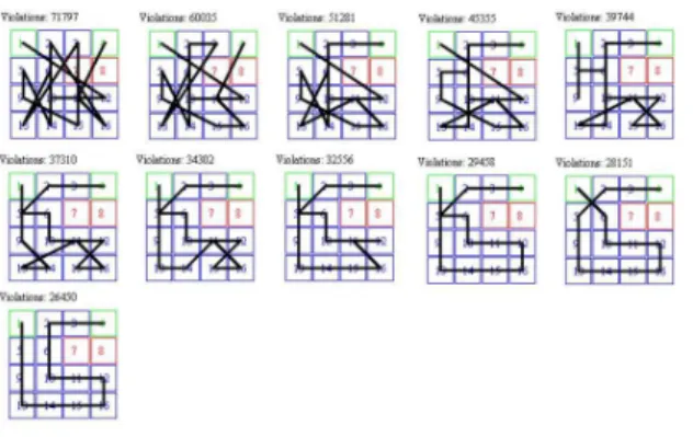
Figure 4.8: The same field instance at different moments in time. The progress occurs

from top to bottom, left to right, with decreasing cost at each step. The route is initialized randomly in the first moment of the progress. Cells 7 and 8 are obstacles and are not covered. Cells 1 and 4 is the start and finish position respectively.

Figure 4.8 illustrates the progress made in one simple instance. The visualizer is constantly looking for new routes in the text file populated by the planner and is updated immediately after a new solution is found. In some situations, it can be configured to display only the best solution until some moment in time (instead of all the small changes being made to a solution), since it is beneficial not to overload the file with all the minimal changes that are being made. Additionally, the visualizer has the ability to save the best route and violations as an image file, autonomously. As a side note, although in the first four pictures of Figure 4.8may appear that the drone flies over an obstacle, the actual path is rather implicit (it takes the shortest path from one cell to another bypassing the obstacles). In other words, the route that is displayed in the image is a shorter version than the actual route. For example, the second sub-figure shows that the route travels from cell 11 to the cell 4, the finishing cell, when in fact it actually travels to cell 4 passing through cell 6 and 2, bypassing the obstacles. This will be formally described in Section

5.3.

4.4 Tools

The coverage path planner was developed using Comet, a programming language de-signed by Pascal Van Hentenryck and Laurent Michel used to solve complex combinatorial optimization problems in areas such as resource allocation and scheduling. As referred in [13], it off_{ers a range of optimization algorithms: from mathematical programming to}

constraint programming, local search algorithm and “dynamic stochastic combinatorial optimization”. Comet programs specify local search algorithms as two components:

• A high-level model describing the applications in terms of constraints, constraint combinators, and objective functions;

4 . 4 . T O O L S

• A search procedure expressed in terms of the model at a high abstraction level.

Its API allows it to be used as a software library. Comet also features high-level abstractions for parallel and distributed computing, based on loop scheduling, interrup-tions, and work stealing. Regarding the interface of the system, Google Maps services was used with JavaScript and HTML to build a user-friendly interface that lets the user select the desired crops, obstacles and start/end cells to provide to the planner. Java was used to build the planner visualizer. Additionally, other tools may be explored such as OscaR which is a Scala toolkit for solving Operation Research problems and include Constrained Based Local Search techniques.

C

h

a

p

t

e

r

5

C o v e r a g e Pa t h P l a n n e r

5.1 Description

The coverage path planner is the component that is iteratively searching for new and improved solutions to some provided instance. This planner considers the elevation of the terrain and the amplitude of the curves made throughout the path. The next sub sections describe the approach that was taken to build this planner, including the problem modeling and the necessary implementation steps.

5.2 Problem Modeling

The problem modeling follows a similar approach of [9] described earlier in the related work section, which is a good example to follow and a convenient basis to start from. As mentioned, there are some distinctions between this thesis and the work by Modares. The first being the fact that this dissertation considers the steepness of the terrain, and the second distinction is that this system allows the user to choose different starting/finishing

points for the route.

The area to be swept by the drone is represented as a set of grid cells, or nodes, and it is assumed that a grid cell is covered when the drone visits its center. The grid is represented as a graph G(V_,E) where Vis the set of nodes and Eis the set of edges. We

leti, j, k ∈ Vdenote a specific node and_e

ij ∈ Edenote an edge between nodesi andj.

Also, there may exist a set of obstacles Ksuch thatK_⊂ V. We’ll also assume that the

drone always traverses adjacent cells, therefore there will only be edges from one cell to adjacent cells. Figure 5.1illustrates a simple field represented as a graph.

Denoting (xi, yi, zi) as the Cartesian coordinate of nodei, one can now define a cost

function which considers the Euclidian Distance between two cells, as in equation5.1.

C H A P T E R 5 . C OV E R AG E PAT H P L A N N E R

Figure 5.1: Example of an area to be swept represented as a oriented graph. The black node is an obstacle. The graph is oriented since the difference in altitudes are considered.

d(i, j) =

         q

(x_i−x_j)2_{+ (y}

i−yj)2+ (zi−zj)2, ifeij∈Eandi, j<K

∞, otherwise

(5.1)

With the cost of distances defined, we now need to include the variation of altitude, or elevation costs. To explain the influence of altitude variation, we can imagine having two adjacent cells where the distance between the two cells is the same regardless of the direction it is taking (from A to B or from B to A) but going into higher grounds will have higher impacts in the power consumption, and therefore should cost more. The altitude variation cost function is defined in equation 5.2.

h(i, j) = 1 +kh(zj−zi) d(i, j)

!2

(5.2)

Wherezj is the altitude of the destination cell, andzi the altitude of the current cell.

The term kh denotes the weight associated with the altitude variation. By having this

parameter set to 0, the altitude variation cost has no influence in the overall cost.

As described in [9] we’ll also consider the amplitude of the curves made throughout the path. The higher the amplitude made in each turn, more power consumption the drone will consume, which is something we want to minimize as well. Turns vary in 45, 90, 135 and 180 degrees, depending on where the drone is coming from and where it is going to (Figure 5.2). Denotingθijk as the exterior angle between nodesi, j, k∈ V. The

squared length of the edges of the triangle made by nodes i, j, k can be determined as defined in equation 5.3.

r= (xi−xj)2+ (yi−yj)2,

s= (xj−xk)2+ (yj−yk)2,

t= (xk−xi)2+ (xk−xi)2

(5.3)

Given the lengths of three sides of the triangle, we can calculate an internal angle using the Law of Cosines. The exterior angle between nodesi, j, k∈ Vcan be written as

shown in equation 5.4.

θijk=π−arccos

"

r+s−t

√

4rs

#

radians (5.4)

5 . 3 . I M P L E M E N TAT I O N

Figure 5.2: A cell and its neighbors, and the exterior angle for three nodes on the path

The termθijkis defined in radians, the conversion to degrees is obtained with equation 5.5

angle(i, j, k) =

         180

π θijk ifeij, ejk∈E

∞, otherwise

(5.5)

Now that we know how to calculate the angles given any three nodes, we can define a cost penalization (equation 5.6).

a(i, j, k) = 1 +ka×angle(i, j, k) 180

!2

(5.6)

The termk_asets the weight associated with the cost of the angle. With this parameter set to 0, the cost of the angle has no influence in the overall cost. What was mentioned until now in this section, models the problem considering three points:

1. The cost of moving the drone from one point to another, considering the distance and the altitude change, where going to higher grounds will have higher impacts in the cost than going downwards.

2. The cost of performing high degree turns, the higher the amplitude of the curve, costlier will be.

3. The obstacles, where the cost from one cell to some obstacle cell is infinity.

5.3 Implementation

In this section, the equations defined in the previous section related to the three com-ponents (distance, altitude and angles) are combined to create a cost system and then further plugged into the coverage path planner. The execution of the planner consists of these seven steps:

1. Reading an instance.

2. Adjacency cost matrix (cost of distances).

C H A P T E R 5 . C OV E R AG E PAT H P L A N N E R

3. Floyd-Warshall’s algorithm (shortest path between all pairs of nodes).

4. Overall cost matrix (include the penalization of angles and altitudes).

5. Model the planner constraints.

6. Route initialization.

7. Local Search.

Step 1- Reading an instance

The first step the planner must take is to read an instance. A very simple example of the file structure is shown in Listing 5.1which creates a field shown in Figure 5.3.

Listing 5.1: File structure

1 2 4

2 1 4

3 2

4 2

5 3

6 200.24 201.50 202.23 203.24 7 201.34 202.25 203.50 204.12

Each row is listed and described as follows:

1. The number of rows and columns (2 4).

2. The start and end cell (1 4).

3. Number of blocked cells (2).

4. First blocked cell (2).

5. Second blocked cell (3).

6. Elevations of the first row for each column in meters.

7. Elevations of the second row for each column in meters.

(a) Field (b) Elevations

Figure 5.3: The field (a) and the elevations of each cell (b). The start cell is 1 and the finish cell is 4.

5 . 3 . I M P L E M E N TAT I O N

Step 2 - Adjacency cost matrix (cost of distances)

From an implementation point of view, the graph can be represented as ann bym matrix, M, where both rows and columns are uniquely identified by a number from

1,2. . . , nand 1,2. . . , m, respectively. Each entry of the matrix M, denoted by_uij is the

cost of going from cell i toj. This second step of the implementation process follows the example shown in Figure 5.4and consists in populating the adjacency cost matrix (Table 5.1) with the costs of distances. As the name suggests, only the adjacent cells and respective entries are populated with the costs of distances.

Figure 5.4: A very small example of an area to be swept with one obstacle (cell 6).

1 2 3 4 5 6

1 0 d(1,2) ∞ d(1,4) d(1,5) ∞

2 d(2,1) 0 d(2,3) d(2,4) d(2,5) ∞

3 ∞ d(3,2) 0 ∞ d(3,5) ∞

4 d(4,1) d(4,2) ∞ 0 d(4,5) ∞

5 d(5,1) d(5,2) d(5,3) d(5,4) 0 ∞

6 ∞ ∞ ∞ ∞ ∞ ∞

Table 5.1: The adjacency cost matrix.

Table 5.1shows the costs of moving from cellito cellj. Eachd(i, j) is defined using equation 5.1. As defined in the equation, we can see from the adjacency cost matrix that the cost is infinity when going from one cell to another that is not adjacent. Additionally, every cell that goes to or from cell 6 (obstacle) is also set to infinity.

Step 3 - Floyd Warshall’s algorithm (shortest path between all pairs of nodes)

Now that the adjacency cost matrix has been calculated, the Floyd-Warshall’s algo-rithm [14] is run to obtain the shortest path between any two nodes in the graph. This step also leaves us with an updated matrix (Table 5.2) where the previous entries of non-adjacent cells are now populated with the corresponding costs. For example, the entryu1,3is now defined asd(1,3) since the algorithm gave us the shortest path between

the two nodes. In this case,d(1,3) =d(1,2) +d(2,3).

C H A P T E R 5 . C OV E R AG E PAT H P L A N N E R

Listing 5.2: Floyd-Warshall’s algorithm

1 function S = floyd (M) 2 S = M;

3 n = size (S ,1);

4 for i = 1:n S(i,i) = 0; end 5 for k = 1:n

6 for i = 1:n 7 for j = 1:n

8 if S(i,k) + S(k,j) < S(i,j) 9 S(i,j = S(i,k) + S(k,j);

10 return S;

Listing 5.3: Floyd-Warshall’s algorithm updated

1 function [S, Next ] = floyd (M) 2 S = M;

3 n = size (S ,1); 4 for i = 1:n 5 for j = 1:n 6 Next (i,j) = j 7 for k = 1:n 8 for i = 1:n 9 for _{j = 1:n}

10 if S(i,k) + S(k,j) < S(i,j) 11 S(i,j = S(i,k) + S(k,j); 12 Next (i,j) = Next (i,k);

13 return S;

To better understand the Floyd-Warshall’s algorithm, a brief explanation is given, starting with the basic form of the algorithm shown in Listing 5.2.

The algorithm is described next. Note that the variables defined in this description are refereed only to the variables specified in the code from Listing 5.2.

1. Initialize a matrixS of shortest paths with the adjacency matrix (the matrix calcu-lated in the previous step). Nodes that are not adjacent have infinity cost in the corresponding matrix entry.

2. For all values k from 1 to niterate. On iteration k, update S, by considering all indirect paths passing through nodek.

3. After the last iteration the costs of distances between any two nodes in the graph are stored in matrixS and returned.

This algorithm only computes the costs (distances) of the shortest paths between any two nodes but does not return the actual paths. To find these paths we first need to start by adding a little bit of code. Listing 5.3shows us the updated code.

5 . 3 . I M P L E M E N TAT I O N

Listing 5.4: Path reconstruction

1 function P = path (u,v, Next ) 2 if N(u,v) == inf

3 P = [];

4 return;

5 end

6 P = [u];

7 while u != v

8 u = Next (u,v); 9 P = [P,u];

10 end

11 end

Now, we have included the matrixN ext(as in next node). This matrix is initialized withj, i.e. it assumes that a direct path fromi toj with no intermediate nodes is the best choice (so far). Then, in the inner loop of the Floyd-Warshall’s algorithm, if a new shortest path is found, the new leading arc is updated accordingly. The finalN extmatrix basically tells us that, if we wish to go from cellAtoB, then we must start the path by first going into cellC. Consequently, there is still a piece of code missing, which is the code that reconstructs the entire path of going from one cell to another. This code is shown in Listing 5.4

The code in Listing 5.4shows us that the path between any two nodesu andv, can be obtained by following the trail indicated in matrixN ext. The first test checks whether there is an actual path between nodesu andv. If there is a path, then the reconstruction begins, starting in nodeu.

1 2 3 4 5 6

1 0 d(1,2) d(1,3) d(1,4) d(1,5) ∞

2 d(2,1) 0 d(2,3) d(2,4) d(2,5) ∞

3 d(3,1) d(3,2) 0 d(3,4) d(3,5) ∞

4 d(4,1) d(4,2) d(4,3) 0 d(4,5) ∞

5 d(5,1) d(5,2) d(5,3) d(5,4) 0 ∞

6 ∞ ∞ ∞ ∞ ∞ ∞

Table 5.2: The updated cost matrix.

Step 4 - Overall cost matrix (include the penalization of angles and altitudes)

In step 2, the cost matrixMwas populated with the adjacency distance costs. Then in

step 3, this matrix was used to execute the Floyd Warshall’s algorithm, which gave us the shortest path between any two nodes in the graph. Having these shortest paths, we can now update our matrix to include both the altitude variation costs and the cost relative

C H A P T E R 5 . C OV E R AG E PAT H P L A N N E R

to the amplitude of the curves made throughout the path. Therefore, this fourth step consists in updating the previous matrix with the costs just mentioned.

Given the shortest path between any two cells of the grid (nodesaandb, for example), let’s denote the path between these two nodes as a sequence ofrcells,P_ab, where each cell ofPab is defined aspi and 1≤i≤r. p1is the start node (a) andpr the finish node (b) of

the path sequencePab. With this notation, the termsd(a, b) from Table 5.2are updated

tot(a, b) using the formula shown in equation 5.7.

t(a, b) =

r−1

X

i=1

d(pi, pi+1)×h(pi, pi+1)×a(pi−1, pi, pi+1), such thatpi∈Pab (5.7)

The total cost matrix is then completed and can now be used by the planner. To exemplify, let’s try to obtain the cost of going from cell 3 to cell 4. The shortest path sequence from node 3 to 4 is:P3,4= (3,5,4). Equation 5.7breaks down into the following

segments:t(3,4) =d(3,5)×h(3,5)×a(0,3,5) +d(5,4)×h(5,4)×a(3,5,4). We assume thatp0

is a virtual previous point so that everya(p0, x, y) equals 1.

Step 5 - Building the Model

Comet allows us to build a constraint system that helps the planner obtain better solutions, measured by the degree of violations of the specified constraints. By imposing a constraint that the cost should be zero, the solver indirectly minimizes the cost by minimizing the constraint violation. Having in mind that a solution is a sequence of steps between cells, the overall constraint violation is the sum of the violations of the individual steps (each constrained to have zero cost). When the steps involve non-contiguous cells, care must be taken regarding the penalization of the curves. For example suppose we ended up with the solution (1,3,5,4,2) for the field of Figure 5.4. In this case the angle to be considered when going from cell 3 to 5 must take into account that the drone comes from cell 2 and not cell 1.

Figure 5.5: A non optimal solution. The path taken from cell 1 to 3 is through cell 2. From 3 to 5 is direct since they are adjacent.

Step 6 - Route initialization

Every local search procedure must start with some solution. Therefore, two distinct heuristics were used and compared for the initial route:

5 . 3 . I M P L E M E N TAT I O N

1. Randomized: The initial route is completely randomized.

2. Field Sweep: The initial route sweeps the area horizontally or vertically along the longest dimension.

Step 7 - Local Search

With everything set up, the local search is initialized. For this step, all three meta-heuristics described earlier in Section 3.2were used and tested, but for Tabu andVNS

a very small change was made regarding its implementation, as described next. Local search selects, at each iteration, two cells to swap and change routes. This is the well-known 2-opt algorithm which was adopted in this dissertation. As described in [12] the main idea behind 2-opt is to take a route that crosses over itself and reorder it so that it no longer does. For example, if the current solution for some basic field is (1,4,6,7,9) and cells 4 and 9 are selected, then the changed and improved solution will be (1,9,7,6,4). All the cells between 4 and 9 are also mirrored to the opposite side. The cell selection step may be performed in various ways. The ideal way is to select two cells that minimize the overall cost, but this can be very costly in terms of computational time because the minimum of all possible combinations must be found. A faster approach consists of first randomly selecting one cell and then select the second cell that minimizes the cost. This helps to detect a wider variety of solutions faster but may be harder to find the optimal solution, and at some iterations an improvement may not even be found because the selection of the first cell was not adequate. The adapted VNS is basically the same as the original but with changes regarding the cell selection. It consists of performing the first type of cell selection (two cells that minimize the cost), and if the time that took to select those two cells passes some pre-defined threshold, then the selection type will change for the next iterations to the second type (first select a random cell, then select a second one that minimizes). As it was mentioned, using this second type of selection may lead to iterations where no improvement was made at all, not because it reached a local optimum, but because the first randomly selected cell did not lead to any further improvements, while there may be other cells that would. For this reason, a new variable was added only for the second type of cell selection. This variable is called the fail streak variable. If no improvements were made in the current iteration the fail streak is increased until it reaches the maximum streak. After it has reached the maximum streak, the normal VNS diversity method is applied. Regarding Tabu Search, it follows the same cell selection principle as the adapted VNS, the rest of the algorithm is the same as described in Section

3.2. SAdoesn’t need to find two cells that minimize the costs, it evaluates some neighbor solution and decides whether it should accept it or not, hence, this fail streak variable is not necessary.

C H A P T E R 5 . C OV E R AG E PAT H P L A N N E R

5.4 Scaling the planner

The problem of executing local search in much bigger instances is the search space itself and the time it takes to find the solution. It’s just not viable to feed the solver with such big instances. Therefore, a technique was prepared that breaks down the main problem (a very big instance/field) into smaller problems (smaller instances/fields). This technique consists of creating sub-areas from the initial field as shown in Figure 5.6

(a) Field (b) Sub-areas

Figure 5.6: The field instance from the paper chosen as a benchmark [9] with obstacles as grey cells. On the left the normal field and at the right all the 8 sub-areas generated delimited as diff_{erent shades of green.}

The algorithm starts by selecting an unexplored node (let’s say cell 1) and expands diagonally at each step. When the expansion reaches cell 19, the area has the dimension-ality of 3x3 units. From there, it detects that it can no longer expand diagonally because of the obstacle in cell 20 and, as such, it should continue expanding vertically, to cell 27, concluding a new area of 4x3 units. This process is repeated until all cells are explored. The purpose of this is to create a planner for every generated sub-area. The solutions of each area would need to be merged in such way that the end point of one sub-area matches the start point of the next. Only the sub-area generation was developed, hence, the technique was not integrated with the current planner, and is left out as future work.