ROMAN BAJIREANU
REAL-TIME HUMAN BODY DETECTION AND
TRACKING FOR AUGMENTED REALITY MOBILE
APPLICATIONS
Master Thesis in Electric and Electronics Engineering Specialisation in Information Technology and Telecommunications
Developed under the orientation of: Professor Doutor João Miguel Fernandes Rodrigues Professor Doutor Pedro Jorge Sequeira Cardoso
UNIVERSITY OF ALGARVE
REAL-TIME HUMAN BODY DETECTION AND TRACKING
FOR AUGMENTED REALITY MOBILE APPLICATIONS
Declaração de autoria de trabalho
Declaro ser o autor deste trabalho, que é original e inédito. Autores e trabalhos con-sultados estão devidamente citados no texto e constam da listagem de referências in-cluída.
I hereby declare to be the author of this work, which is original and unpublished. Authors and works consulted are properly cited in the text and included in the reference list.
©2018, ROMAN BAJIREANU
A Universidade do Algarve reserva para si o direito, em conformidade com o dis-posto no Código do Direito de Autor e dos Direitos Conexos, de arquivar, reproduzir e publicar a obra, independentemente do meio utilizado, bem como de a divulgar através de repositórios científicos e de admitir a sua cópia e distribuição para fins meramente educacionais ou de investigação e não comerciais, conquanto seja dado o devido crédito ao autor e editor respetivos.
The University of the Algarve reserves the right, in accordance with the terms of the Copy-right and Related Rights Code, to file, reproduce and publish the work, regardless of the meth-ods used, as well as to publish it through scientific repositories and to allow it to be copied and distributed for purely educational or research purposes and never for commercial purposes, provided that due credit is given to the respective author and publisher.
Acknowledgements
I would like to thank my supervisor João Rodrigues for suggesting the topic and for guidance. Similar, thank to my secondary supervisor Pedro Jorge Sequeira Cardoso for being dedicated to his role. Thanks also go to Roberto Lam for the help during various stages of the project.
I also would like to thank all my close friends and lab colleagues for their support, words of encouragement, shared knowledge and patience.
Last but not least, I would like to thank my family, my parents Toma and Olga and my brother Adrian, for their unconditional support, encouragement, and love, without which I would not have come this far.
Resumo
Hoje em dia, cada vez mais experiências culturais são melhoradas tendo por base cações móveis, incluindo aqueles que usam Realidade Aumentada (RA). Estas apli-cações têm crescido em número de utilizadores, em muito suportadas no aumento do poder de cálculo dos processadores mais recentes, na popularidade dos dispositivos móveis (com câmaras de alta definição e sistemas de posicionamento global – GPS), e na massificação da disponibilidade de conexões de internet. Tendo este contexto em mente, o projeto Mobile Five Senses Augmented Reality System for Museums (M5SAR) visa desenvolver um sistema de RA para ser um guia em eventos culturais, históricos e em museus, complementando ou substituindo a orientação tradicional dada pelos guias ou mapas. O trabalho descrito na presente tese faz parte do projeto M5SAR. O sistema completo consiste numa aplicação para dispositivos móveis e num dispositivo físico, a acoplar ao dispositivo móvel, que em conjunto visam explorar os 5 sentidos humanos: visão, audição, tato, olfacto e paladar.
O projeto M5SAR tem como objetivos principais (a) detectar peças do museu (por exemplo, pinturas e estátuas (Pereira et al., 2017)), (b) detectar paredes / ambientes do museu (Veiga et al., 2017) e (c) detectar formas humanas para sobrepor o conteúdo de Realidade Aumentada (?). Esta tese apresenta uma abordagem relativamente ao úl-timo objectivo, combinando informações de articulações do corpo humano com méto-dos de sobreposição de roupas.
Os atuais sistemas relacionados com a sobreposição de roupas, que permitem ao utilizador mover-se livremente, são baseados em sensores tridimensionais (3D), e.g., Sensor Kinect (Erra et al., 2018), sendo estes não portáteis. A contribuição desta tese é apresentar uma solução portátil baseado na câmara (RGB) do telemóvel que permite ao utilizador movimentar-se livremente, fazendo ao mesmo tempo a sobreposição de roupa (para o corpo completo).
Nos últimos anos, a capacidade de Redes Neurais Convolucionais (CNN) foi com-provado numa grande variedade de tarefas de visão computacional, tais como classi-ficação e detecção de objetos e no reconhecimento de faces e texto (Amos et al., 2016; Ren et al., 2015a). Uma das áreas de uso das CNN é a estimativa de posição (pose) humana em ambientes reais (Insafutdinov et al., 2017; Pishchulin et al., 2016). Re-centemente, duas populares CNN frameworks para detecção e segmentação de formas humanas apresentam destaque, o OpenPose (Cao et al., 2017; Wei et al., 2016) e o Mask R-CNN (He et al., 2017). No entanto, testes experimentais mostraram que as imple-mentações originais não são adequadas para dispositivos móveis. Apesar disso, estas frameworks são a base para as implementações mais recentes, que possibilitam o uso em dispositivos móveis. Uma abordagem que alcança a estimativa e a segmentação de pose de corpo inteiro é o Mask R-CNN2Go (Jindal, 2018), baseado na estrutura origi-nal do Mask R-CNN. A principal razão para o tempo de processamento ser reduzido foi a otimização do número de camadas de convolução e a largura de cada camada.
Outra abordagem para obter a estimativa de pose humana em dispositivos móveis foi a modificação da arquitetura original do OpenPose para mobile (Kim, 2018; Solano, 2018) e sua combinação com MobileNets (Howard et al., 2017). MobileNets, como o nome sugere, é projetado para aplicativos móveis, fazendo uso de camadas de con-voluções separáveis em profundidade. Essa modificação reduz o tempo de proces-samento, mas também reduz a precisão na estimativa da pose, quando comparado à arquitetura original.
É importante ressaltar que apesar de a detecção de pessoas com a sobreposição x
de roupas ser um tema atual, já existem aplicações disponíveis no mercado, como o Pozus (GENTLEMINDS, 2018). O Pozus é disponibilizado numa versão beta que é executado no sistema operativo iOS, usa a câmera do telemóvel como entrada para a estimação da pose humana aplicando segmentos de texturas sobre o corpo humano. No entanto, Pozus não faz ajuste de texturas (roupas) à forma da pessoa.
Na presente tese, o modelo OpenPose foi usado para determinar as articulações do corpo e diferentes abordagens foram usadas para sobreposição de roupas, enquanto uma pessoa se move em ambientes reais. A primeira abordagem utiliza o algoritmo GrabCut (Rother et al., 2004) para segmentação de pessoas, permitindo o ajuste de seg-mentos de roupas. Uma segunda abordagem usa uma ferramenta bidimensional (2D) de Animação do Esqueleto para permitir deformações em texturas 2D de acordo com as poses estimadas. A terceira abordagem é semelhante à anterior, mas usa modelos 3D, volumes, para obter uma simulação mais realista do processo de sobreposição de roupas. Os resultados e a prova de conceito são mostrados.
Os resultados são coerentes com uma prova de conceito. Os testes revelaram que como trabalho futuro as otimizações para melhorar a precisão do modelo de estimação da pose e o tempo de execução ainda são necessárias para dispositivos móveis. O método final utilizado para sobrepor roupas no corpo demonstrou resultados posi-tivos, pois possibilitaram uma simulação mais realística do processo de sobreposição de roupas.
Palavras chave: Redes Neurais Convolucionais, Estimação de Pose, Sobreposição de Roupas, Inteligencia Artificial.
Abstract
When it comes to visitors at museums and heritage places, objects speak for them-selves. Nevertheless, it is important to give visitors the best experience possible, this will lead to an increase in the visits number and enhance the perception and value of the organization. With the aim of enhancing a traditional museum visit, a mobile Augmented Reality (AR) framework is being developed as part of the Mobile Five Senses Augmented Reality (M5SAR) project. This thesis presents an initial approach to human shape detection and AR content superimposition in a mobile environment, achieved by combining information of human body joints with clothes overlapping methods.
The present existing systems related to clothes overlapping, that allow the user to move freely, are based mainly in three-dimensional (3D) sensors (e.g., Kinect sensor (Erra et al., 2018)), making them far from being portable. The contribution of this thesis is to present a portable system that allows the user to move freely and does full body clothes overlapping.
The OpenPose model (Kim, 2018; Solano, 2018) was used to compute the body joints and different approaches were used for clothes overlapping, while a person is moving in real environments. The first approach uses GrabCut algorithm (Rother et al., 2004) for person segmentation, allowing to fit clothes segments. A second ap-proach uses a bi-dimensional (2D) skeletal animation tool to allow deformations on
2D textures according to the estimated poses. The third approach is similar to the pre-vious, but uses 3D clothes models (volumes) to achieve a more realistic simulation of the process of clothes superimposition. Results and proof-of-concept are shown.
Keywords: Convolutional Neural Network, Pose Estimation, Clothes Overlap-ping, Artificial Intelligence.
Table of Contents
List of Figures . . . xvi
List of Abbreviations . . . xix
Chapter 1 Introduction . . . . 1
1.1 Scope of the Thesis . . . 2
1.2 Objectives . . . 3
1.3 Overview of the Thesis . . . 4
Chapter 2 Contextualization and State-of-the-art . . . . 5
2.1 Introduction . . . 5
2.2 Neural Networks . . . 7
2.2.1 Convolutional Neural Networks . . . 9
2.3 Person Detection . . . 13
2.3.1 Haar Cascades . . . 13
2.3.2 Histogram of Oriented Gradients . . . 15
2.3.3 Convolutional Neural Networks Methods . . . 17
2.4 Pose Estimation . . . 21
2.4.1 OpenPose . . . 22
2.5 Clothes Overlapping . . . 24
2.6 Discussion . . . 26
Chapter 3 Clothes Overlapping . . . . 29
3.1 Introduction . . . 29 3.2 Pose estimation . . . 30 3.3 Clothes Overlapping . . . 32 3.3.1 Segments . . . 32 3.3.2 Textures . . . 36 3.3.3 Volumes . . . 39 3.4 Discussion . . . 41
Chapter 4 Conclusions and Future Work . . . . 43
4.1 Conclusion . . . 43
4.2 Future work . . . 45
4.3 Publications . . . 45
Appendix A GrabCut . . . . 47
List of Figures
2.1 Example of an artificial neuron. Adapted from (Pokharna, 2018). . . 8
2.2 Example of a fully-connected multi-layer neural network. . . 8
2.3 An example of a convolution layer with two filters, each with a spatial extent of 3, moving at a stride of 2, and input padding of 1. Adapted from (cs231n, 2018). . . 11
2.4 Pooling operations. Top, max pooling and bottom, average pooling. The filters and stride size is 2. . . 12
2.5 Cascade classifiers. . . 14
2.6 Haar-like features. . . 14
2.7 Haar Cascades detection output. A rectangle is blue, green, red and black for full body, upper body, lower body, and face, respectively. . . . 15
2.8 Histogram orientation gradient process. Adapted from (Dalal and Triggs, 2005) . . . 16
2.9 Histogram of oriented gradients output. A green rectangle represents a detection. An image without a green rectangle has no detections. . . 16
2.10 Stages of R-CNN forward propagation. Adapted from (Girshick et al., 2014). . . 17
2.11 Fast R-CNN architecture. Adapted from (Girshick, 2015). . . 18
2.12 Faster R-CNN workflow. Adapted from (Ren et al., 2015b). . . 19
2.13 SSD architecture. Taken from (Huang et al., 2017). . . 20
2.14 SSD-Mobilenet output. A green rectangle represents a detection. . . 21
2.15 OpenPose pipeline. Adapted from (Cao et al., 2017). . . 22
2.16 Architecture of the two-branch multi-stage CNN. Adapted from (Cao et al., 2017). . . 23
2.17 OpenPose pipeline, followed by an image. Adapted from (Kim, 2018). . 25
3.1 Examples of pose estimation. . . 30
3.2 Top row, example of confusion between left and right ankle (left) and a well detected pose (right). Bottom row, example of pose estimation with spatial size of the CNN equal to 368×368px (left) and 184×184px (right). . . 31
3.3 Examples of the clothes segments. . . 33
3.4 Top row, limb’s angle (left), and the distances calculated to fit the clothes (right). Bottom row, segment stretch directions (left), and final result (right) (see Sec. 3.3.1). . . 34
3.5 Top row, example clothes overlapping. Middle row, example of a bound-ing box (left) and segmentation (right). Bottom row, projection of
con-tents on person body after clothes fitting. . . 35
3.6 Sequence of frames of a human shape superimposition using “segmen-tation”. . . 37
3.7 Example of created bones. . . 38
3.8 Example of human shape superimpostion using “textures”. . . 38
3.9 Example of four volume 2D views. . . 39
3.10 Example of volume keypoints. . . 40
3.11 Example of human shape superimpostion using “volumes”. . . 41
A.1 Example of GrabCut approach. Adapted from OpenCv (2018). . . 49
A.2 Grab Cut segmentation output. A green rectangle represents a detec-tion. . . 49
List of Abbreviations
CNN Convolutional Neural Network CPU Central Processing Unit
FPS Frames Per Second
GPU Graphics Processing Unit
R-CNN Convolutional Neural Network with Region proposals RoI Region of Interest
RPN Region Proposal Network SSD Single Shot MultiBox Detector SVM Support Vector Machine
HSS Human Shape Superimposition M5SAR Mobile 5 Senses Augmented Reality App Mobile Application
AR Augmented Reality ML Machine Learning
1
Introduction
Imagine a visit to a museum where you can see, hear, feel, smell and maybe even taste what existed when the museological pieces were developed or what is represented in them. This would be a step towards a more immersive experience when compared to the traditional guides existing in most museums. In this context, this dissertation pro-poses the development of a Human Shape Superimposition (HSS) module for a mul-tiplatform Augmented Reality (AR) application (App) for mobile devices (Android, iOS, and Windows). The application will be used within buildings and aims to serve as a guide in cultural, historical and museological events. The application’s devel-opment is a module in the M5SAR project: Mobile Five Senses Augmented Reality System for Museums (for more details see Sec. 1.1).
The HSS module projected in this thesis will do human shape detection and AR content (clothes) superimposition, achieved by combining information of human body joints with textures/volumes representing the clothes.
The existing texture overlapping methods for mobile devices are mainly limited to frontal body view and do not allow the user to move freely (Martin and Oruklu, 2012; Shaikh et al., 2014). These methods are based on face detectors (e.g., Haar cas-cades (Viola and Jones, 2001)) and markers (e.g., tags or images; a.k.a. marker-based). However, they mainly try to explore the virtual dressing room concept, providing an experience to virtually check the clothes fit or the style.
This dissertation also explores the use of Machine Learning (ML) methods to de-tect human shapes, in order to overlay different clothes over those shapes. The main intention is to detect human shapes in real-time on a mobile device, while the user is moving freely.
1.1
Scope of the Thesis
The work presented in this thesis is a part of the M5SAR project products, funded by Portugal2020, CRESC Algarve 2020 I&DT, n° 3322, promoter SPIC - Sonha Pensa Imagina Comunica, Lda.1 and co-promoter University of the Algarve 2. The project started in January 2016 and finished in October 2018.
In summary, the project aimed to develop an AR system, consisting of an applica-tion platform and a device (here referred to as “gadget”) to be integrated with mobile devices (phablets and tablets) that explore the 5 human senses (5S) (vision, hearing, touch, smell, and taste). The project solutions focus on being used as a guide in cul-tural, historical and museum events. The system consists of three products, to be used integrated or individually, as explained next. First a (a) software Application for mo-bile devices, that will be available in the “app store” or on a website, works on the
1http://spic.pt/ 2http://www.ualg.pt/
latest phablet and tablet devices, focusing on 4 of the 5 senses namely: sight, hear, touch and taste. The second product consists of a (b) hardware device that can be sold separately or rented at the museum. This device focuses on 3 of the 5 senses: touch, smell and taste. Finally, the (c) association of the App, (a), and the device, (b), deep-ening the user experience. For this, the hardware device is able to attach itself to the mobile device, as well as to communicate and be integrated with the App. Together they allow the full integration of the 5 senses in the AR. Each one of these products, in-dividually and especially together are, without a doubt, a novelty in the market since, as far as we now, nothing exists with these settings/specifications. The final product allows a more immersive interaction with the surrounding space than the existing AR systems. To achieve these goal it was necessary to combine research and development in various areas such as Information and Communication Technology (ICT), electron-ics, emotions psychology and design. The applications and equipment include also a large set of usage such as Smart Cities, creative industries and media, tourism, and natural and cultural heritage. By this via, an innovative product for the global market was created. More information and publications about the project can be found on the website of the project3.
The work presented in this thesis focuses on the HSS module of the product (a).
1.2
Objectives
The goal of this work is to build the HSS module, that combines pose estimation and clothes overlapping in a multi-platform mobile device AR application. The mobile device’s built-in camera is used to scan the environment for humans shapes, which are then overlapped with clothes. The existing clothes overlapping systems (Erra et al., 2018), that allow users to move freely, are based in 3D sensors (e.g., Kinect sensor (Erra et al., 2018)), making them not portable. One of the contributions of this thesis is the
presentation of a new portable system that allows the user to move freely and does full body clothes overlapping on a mobile device.
While developing the HSS module three big challenges arise. The first challenge is the human pose estimation while using a mobile device with reasonable accuracy. The second is to do full body clothes overlapping. The third big challenge is to achieve real-time performances on that mobile device.
As a bounding limit, the HSS module should present performances of at least three shapes superimposition per second, while the user is moving freely.
1.3
Overview of the Thesis
In summary, the present chapter introduced the thesis theme as well as the main goal, contributions and scope.
Chapter 2 focuses on the state-of-the-art for person detection, estimation and clothes overlapping. It presents some of the most important developments in these areas and the methods used for this thesis.
Chapter 3 details all the algorithms implemented for the clothes overlapping pro-cess. It discusses the results in terms of accomplishment of the objectives.
Chapter 4 finalises this work with the general conclusions, mentioning how some problems can be fixed in future work, and also presents some publications made dur-ing the course of this work.
2
Contextualization and State-of-the-art
2.1
Introduction
This chapter introduces concepts necessary to understand the content and scope of this thesis, namely concepts of Machine Learning (ML), Neural Networks (NN), person detection (PD), pose estimation (PE) and clothes overlapping (CO). A discussion about the algorithmic choices made for the proposed work is also presented.
Machine Learning can be considered as a set of data analysis method(s) that au-tomates analytical model building (Bishop, 2006). It is often considered a branch of Artificial Intelligence based on the idea that systems can learn from data, identify pat-terns and make decisions with minimal human intervention. Algorithms in ML are
divide in two main groups: supervised learning and unsupervised learning (Goodfellow et al., 2016, pp. 96).
In supervised learning, a set of training data consisting of a set of training examples are annotated or labeled by humans, and provided to the ML system. For example, a set of training images marked with the location and class of relevant objects can be used for object detection (Bishop, 2006, pp. 104-106). The algorithm learns from the labeled data and then predicts the relevant objects of new data. In supervised learning, the most important machine learning tasks are: classification and regression (Goodfel-low et al., 2016, pp.98-99). An example of classification is object recognition that, based on a trained model, labels new data to classes. For regression, instead of class labels, the new data is placed in continuous values. For example, predict the age of a person given her picture.
In unsupervised learning, a structure or relationship between different inputs is dis-covered without a human telling what the correct output should be. One common unsupervised learning task is clustering (Goodfellow et al., 2016, pp.103), which discov-ers groups of similar examples within the inputs.
In classification tasks, if the process of labeling (massive amounts of) data for pervised learning is prohibitively time-consuming and expensive, a combination of su-pervised learning and unsusu-pervised learning can be done, called semi-susu-pervised learning (Chapelle et al., 2009, pp. 1-4). In semi-supervised learning, a portion of the data is la-beled and provided to the ML system. The trained algorithm is then used to label the unlabeled data (called the pseudo-labeling process) to train a more robust algorithm. This approach has the risk of incorrectly labeling data.
As learning algorithm cannot include every possible instance of the inputs, it has to be able to generalize in order to handle unseen data (Bishop, 2006, pp. 2). Sim-ple methods can fail to capture important features, but too comSim-plex methods can do over-fitting by not including important details or noise. Commonly, over-fitting occurs when a complex method is used in conjunction with a too small training data.
quently, it becomes difficult for the model to generalize new examples (validation and test sets) that were not in the training set (Goodfellow et al., 2016, pp.448).
Quality and quantity of errors are used to evaluate the performance of the algo-rithm. To assign a cost to the errors is used a loss function, such as mean squared error, where the difference between the current and desired output is the error (Bishop, 2006, pp. 41).
2.2
Neural Networks
Neural Networks are one of the most popular ML tools (Schmidhuber, 2015). For the scope of this thesis a specific type of NN called Convolutional Neural Network (CNN) is the focus. This section introduces the concept of NN before discussing CNN.
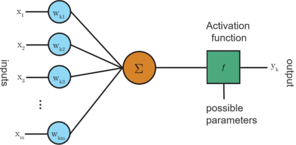
Neural Networks were originally named Artificial Neural Networks because they are computational models inspired by biological systems, such as the way the brain process information. There are mathematical functions that allow to emulate neurons, as the artificial neuron depicted in fig. 2.1. Neuron k receives m input parameters
(x1, x2, ...xm) and has m weight parameters (wk1, wk2, ...wkm). Often, a bias wk0 term,
with a fixed input of 1, is included in the weight parameters. In the process, the linear combination is done between the inputs and weights and an activation function f uses the sum to produce the neuron output yk, i.e.,
yk = f(sk) = f m
∑
j=0 wkjxj+wk0 ! . (2.1)The neuron weights are carefully optimized to produce a desired output for each in-put.
A combination of artificial neurons is a neural network. Layers are used to group neurons. Figure 2.2 shows a fully-connected feed-forward multi-layer network (see Sec. 2.2.1), where each output of a layer of neurons serves as input to each neuron in the next
Figure 2.1: Example of an artificial neuron. Adapted from (Pokharna, 2018).
Figure 2.2: Example of a fully-connected multi-layer neural network.
layer. For example, input layer can serve to pass the data along without modifying it, the hidden layer does the most of the computation and the output layer converts the hidden layer activations to an output, such as classification. As expected in a fully con-nected network, the number of neurons in the previous layer is equal to the number of weights each neuron has (Bishop, 2006, pp. 227-229).
The final output of each neuron is determined using an activation function. A popular activation function is Rectified Linear Units (Goodfellow et al., 2016, pp. 193), which generates the output using an easy to compute ramp function, f(x) =max(0, x). The softmax activation function, given by
σ(z)i =
ezi
∑K j=1ezj
, (2.2)
where i = 1, . . . , K, z is a vector of arbitrary values and K is the size of the vector, 8
is a common function used for multi-class classification problems (Goodfellow et al., 2016, pp.184-187) in the output layer of the network. The softmax function normalizes z into a K dimensional vector σ(z) whose components sum to 1 (in other words, a probability vector), and it also provides a weighted average of each zi relative to the
aggregate of zi’s in a way that exaggerates differences (returns a value close to 0 or 1),
if the zi’s are very different from each other in terms of scale, but returns a moderate
value if zi’s are relatively the same scale. Class probabilities are achieved using the
softmax (see below) output. For other activation functions see (SHARMA, 2017).
2.2.1
Convolutional Neural Networks
Convolutional Neural Networks were inspired by the visual cortex functioning (Fu-kushi ma, 1988). CNN have a feature called receptive fields that contain a complex arrange-ment of receptive neurons and each of those neurons are sensitive to a specific part of the visual field. Every time the eyes see something, the neurons act like local filters that are well-suited to exploit the strong spatially local correlation. There are simple neurons that detect patterns like lines and edges within their receptive area and com-plex neurons that detect patterns that are locally invariant to the exact position of what the eyes saw (Wang, 2013).
In CNN, there are many different architectures. Almost all of them are created from four main types of layers in different combinations: the convolutional layer, the rectified linear units layer (ReLU), the pooling layer and the fully connected layer (cs231n, 2018).
The convolutional layer objective is to extract features of the inputs returning as out-put feature maps (or activation maps). This type of layer has a connection called re-ceptive field that connects each neuron in the feature map to only a local region of the input (previous layer). The receptive field does not look equally to a local region in the input image, but focus exponentially more to the middle of that region. In other words, within a receptive field, the closer a pixel is to the center of the field, the more it contributes to the calculation of the output feature. The process to compute feature
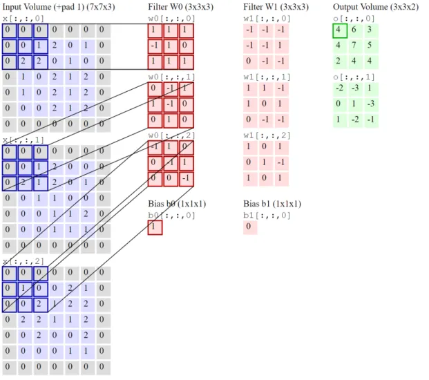
maps (or a forward pass through a convolutional layer) from the input can be done by: first, the designed filter with a local region of the input is convolved. Filters have the same depth as the input. The feature maps are computed by sliding the filters over input data (or map). Figure 2.3 shows an example of a convolution layer. This convo-lution layer applies zero padding, that pads the input volume with zeros around the border. The zero padding allows the design of deeper networks and improves perfor-mance by keeping information at the borders. Filters are slided with a defined stride that has the objective of producing smaller output volumes spatially. A bias term with a fixed size of 1 for first filter and 0 for second filter is included. The bias is a constant that acts as a threshold in ReLU layer for whether a neuron has detected a low-level characteristic.
Usually after each convolution layer is applied the ReLU layer. The rectified lin-ear units layer can be defined as the positive part of its argument: f(x) = max(0, x), where x is the input to a neuron. The convolution layers has just been computing linear operations (just element wise multiplications and summations), but the ReLU layer introduce nonlinearity. In the past, other linear functions were used, but recent researchers found out that ReLU layer works far better because the training process of the network is a lot faster (Goodfellow et al., 2016, pp.174-175). In basic terms, ReLU is linear (identity) for all positive values, and zero for all negative values.
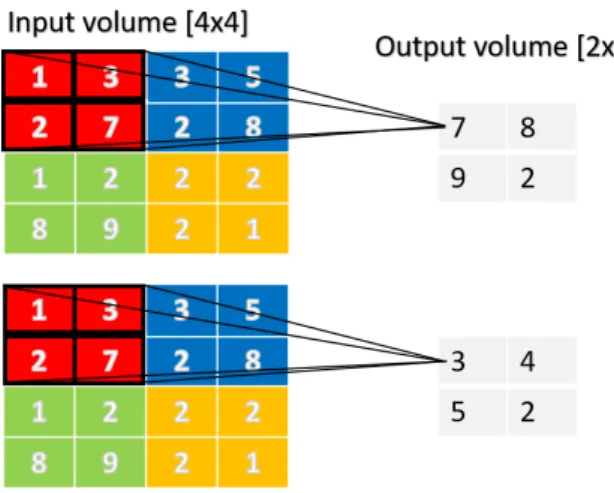
In pooling layer the intuition is that the exact location of a features is not important as its relative location to the other features. This layer lowers the computational com-plexity by reducing the number of parameters in the lower layers. Another effect is control of overfitting. The overfitting is the difficulty for the model to generalize to new examples that were not in the training set. A pooling layer is usually placed be-tween two convolutional layers. There are different pooling operations, but the typical ones are Max pooling and Average pooling (Wang et al., 2012; Boureau et al., 2010). Max pooling takes the maximum value (the value of the brightest pixel) from a feature map. The Average pooling takes the average value from a feature map. Figure 2.4 shows an
Figure 2.3: An example of a convolution layer with two filters, each with a spatial extent of 3, moving at a stride of 2, and input padding of 1. Adapted from (cs231n, 2018).
example of pooling operations.
A fully connected layer takes the high-level filtered images and translates them into votes. A vector of numbers is the input to this layer. This layer connect every neuron in the previous layer (can be convolutional or pooling) to every neuron it has. The output is also a vector of numbers. The output vector of a fully connected layer will be feed to loss layer. The loss layer is normally the final layer and commonly uses a softmax activation function for classification tasks, as it generates a well-formed probability distribution of the outputs (MONCADA, 2018).
A Neural Network learns to approximate target outputs from known inputs by selecting the weights of the neurons. Two techniques can be used to train a CNN, a
Figure 2.4: Pooling operations. Top, max pooling and bottom, average pooling. The filters and stride size is 2.
forward propagation or a backward propagation.
The forward propagation assumes that the convolutional layer output will be of size o = (i− f +2p)/s+1, where o is the output size, i is the input image size, f is the filter matrix size, p is the padding, and s is the stride. Output weights are obtained by the convolution operation. After the convolution operation, the ReLU layer function f(h[x, y]) = max(0, h[x, y])is applied, being h the output feature map from convolu-tional layer. Commonly, pooling layer is the next layer. In case of max pooling, the output dimensionality is obtained the same way as in a convolutional layer. Each2x2
input block is reduced to just a single value via max pooling operation (see Figure 2.4). In a multi-layer network is difficult to solve the neuron weights analytically.
The backward propagation (Goodfellow et al., 2016, pp.204-210) solve the weights iteratively using a simple and effective solution. The classical back-propagation algo-rithm uses the optimization method called gradient descent to find the best weights, i.e., the weights that yield the minimum error. Gradient descent does not guarantee to find the global minimum of loss function and is quite time-consuming, but with proper configuration (hyper-parameters) works well enough in practice (Cui, 2018, pp.5-7). At the first step of the algorithm, in the neural network is propagated forward an input vector. Before this, are initialized the weights of the network neurons. A loss function is used to compare the predicted network output to the desired output.
The gradient of the loss function is then calculated, returning (the loss function is the mean squared error) the difference between the current and desired output, which is the output layer error. To calculate the error values of the hidden layer neurons, the outputted error values are then propagated back through the network. The chain rule of derivatives is used to solve the hidden neuron loss function gradients.
A hyper-parameter called learning rate (Bishop, 2006, pp. 240) is used to control how much the weights of the network are adjusted with respect to the loss gradient. The learning rate can be fixed or dynamic (Bishop, 2006). The neuron weights are updated by multiplying the gradient by the learning rate and subtracting a proportion of the gradient from the weights.
2.3
Person Detection
Three methods were analyzed and then tested for person detection: (a) Haar Cascades (HC), (b) Histogram of Oriented Gradients (HOG) and (c) CNN. The following section presents a brief description of those methods.
2.3.1
Haar Cascades
Haar Cascade (Viola and Jones, 2001) is a ML approach based on the concatenation of simple classifiers that are trained with a large set of object samples. The approach uses a boosted cascade of Haar-like features to process the captured images and detect ob-jects. Boosted means that one strong classifier is created from weak classifiers. In other words, a better classifier is created from a weighted majority vote of weak learners, which depends on only one single feature, consequently increasing the classification performance (Freund et al., 1999).
Haar Cascade has a rejection process, drawn in Fig. 2.5, that contains stages where multiple simple classifiers vote if a region of interest is a accepted sub-window. The earlier stages reject many feature candidates, saving substantial computation time.
Figure 2.5: Cascade classifiers.
Figure 2.6: Haar-like features.
Simple classifiers use as input Haar-like features and a training set of positive and negative sample images. Haar-like features are obtained by subtracting the sum of pixels under the white rectangles from black rectangles. Figure 2.6 shows the types of features. The final detector of different sizes is scanned over the image, extracting features using integral images and applies the trained cascade classifier.
Four already trained detectors (Kruppa and Schiele, 2018) were used for illustration Fig. 2.7: upper body, lower body, full body and frontal face. These detectors deals with frontal and backside views but not with side views. Frontal face detection has a higher accuracy rate when compared with the other detections, because it has to rely on fragile silhouette information rather than internal (facial) features. Figure 2.7 shows
Figure 2.7: Haar Cascades detection output. A rectangle is blue, green, red and black for full body, upper body, lower body, and face, respectively.
some images with the accuracy results presented by drawn rectangles corresponding to the respective detector. From the figure, despite some correct detection, several incorrect detections are observable.
2.3.2
Histogram of Oriented Gradients
Histogram of Oriented Gradients (Dalal and Triggs, 2005) is a feature extraction method based on evaluating over the image a dense grid of normalized local histograms of image gradient vectors. In the first step a preprocessing that reduces the influence of illumination effects is done. Usually, a 2D Gaussian filter is applied over the im-age. In the second step, the horizontal and vertical gradients which captures shape and appearance are calculated. In the third step, local gradient vectors are binned within a spatial grid (called cell) according to their orientations, weighted by magni-tude. Regarding the fourth step, local groups of cells (called block) are normalized. The histogram of gradient vectors from the contributing cells are used to extract a fea-ture vector from each block. In every feafea-ture vector, the individual cell is normalized and shared among several overlapping blocks. In the last step, a Support Vector Ma-chine (SVM) (Girshick et al., 2014) for human detection has as input a final descriptor that is built using collected features vectors from all blocks. A diagram illustrating
Figure 2.8: Histogram orientation gradient process. Adapted from (Dalal and Triggs, 2005)
Figure 2.9: Histogram of oriented gradients output. A green rectangle represents a detection. An image without a green rectangle has no detections.
HOG approach steps is shown in Fig. 2.8.
Figure 2.9 shows some images with the detection results marked with rectangles. As a conclusion the HOG features describes better object outline or shape and the Harr-like features describes better brighter or darker regions. For example, Haar fea-tures works well with frontal faces because the nose bridge is brighter than the sur-rounding face region and HOG performs better with people detection because most prominent features are outlines (or shapes). Nevertheless, the results presented by both approaches are not satisfactory enough to be applied to our problem, so also a CNN based solution was studied and tested, as explained in the next section.
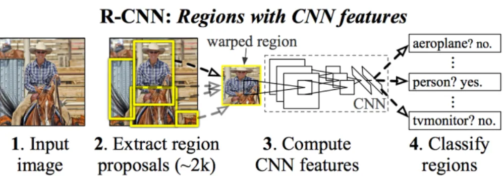
Figure 2.10: Stages of R-CNN forward propagation. Adapted from (Girshick et al., 2014).
2.3.3
Convolutional Neural Networks Methods
This section describes and compares different person detection methods that utilize CNN. The R-CNN (Regions + CNN) (Girshick et al., 2014) method does person detec-tion by using an external region proposal system. A method called Selective Search (Uijlings et al., 2013) is used to generate the regions of interest (RoI), which utilizes an iterative merging of superpixels. To extract features from each region proposal is used a CNN. Each RoI is warped to match the CNN input size and then fed to the network. In the last step, a SVM uses the extracted features from the network to provide the final classification. R-CNN have the following workflow for training: convolutional network training, SVMs fitting to the CNN features and RoIs generating method train-ing. In Girshick (2015) are listed three main problems: (a) training has multiple stages, (b) SVM and region proposal training is expensive because features are extracted from each region proposal and stored on disk, and (c) slow person detection because the forward propagation is done separately for every object proposal. Figure 2.10 shows the R-CNN forward propagation stages.
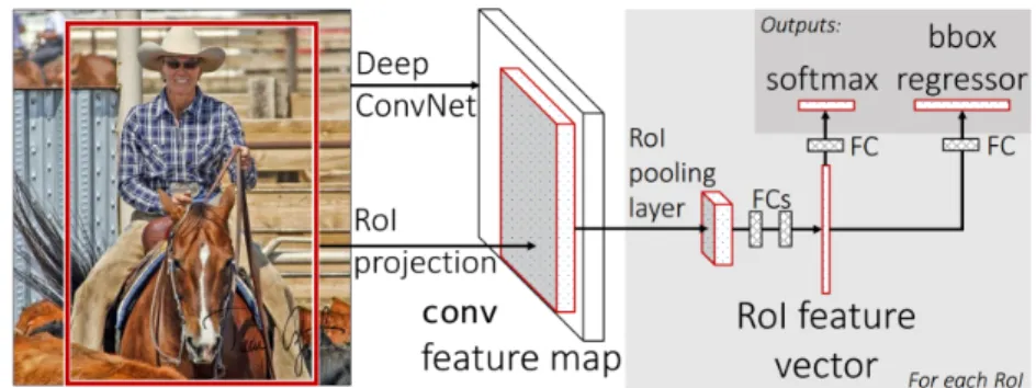
An evolution of the R-CNN is the Fast R-CNN (Girshick, 2015) which creates an unified framework from three methods: feature extractor, classifier and bounding box regressor. The framework receives as input an image plus RoIs generated using an ex-ternal method (selective search). Then the CNN uses several convolutional and max-pooling layers to process the image which outputs a feature map used in a RoI max-pooling
Figure 2.11: Fast R-CNN architecture. Adapted from (Girshick, 2015).
layer. This layer uses the feature map to extract a fixed-length feature vector for each object proposal. A sequence of fully connected layers uses as input the extracted vec-tors. The fully connected layers output is the input to softmax and real-valued layers. A probability distribution of the object classes is the output from the softmax layer. For last in the real-valued layer, a bounding box position is computed for each class using regression (meaning that the initial candidate boxes are refined). Fast R-CNN classi-fication is much faster than R-CNN since each RoI uses the same feature map. The detection time is reduced by around 30% by compressing the fully connected layers using truncated singular value decomposition (Girshick, 2015). As a consequence, the accuracy drops slightly. According to the author, the training time is nine times faster than in R-CNN. The back-propagation algorithm and stochastic gradient descent can be used to train the entire CNN. Figure 2.11 shows the Fast R-CNN architecture.
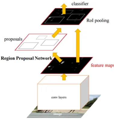
The Faster R-CNN (Ren et al., 2015b) integrates the regional proposal algorithm into the CNN model. The framework consists of two unified CNNs: region proposal network (RPN) that generates the feature proposals and Fast R-CNN structure for the detection network. This CNNs are unified by using a training procedure that al-ternates between training for RoI generation and detection. The first step is to train separately the two networks. In the second step the networks are unified and fine-tuned. During fine-tuning, the shared convolutional layers remain fixed and unique networks layers pass through fine-tuning. In inference, the Faster R-CNN input is a single image. Feature maps generation is done using the shared fully convolutional
Figure 2.12: Faster R-CNN workflow. Adapted from (Ren et al., 2015b).
layers. RPN output region proposals using as input the feature maps. For last, the final detection layers use as input the feature maps and the region proposals to output the final classifications. The integration proposal algorithm into the CNN model has the advantage of being realizable on a GPU. In CPU implementation is used an exter-nal region proposal system. To deal with different scales and aspect ratios detections in the sliding window are used anchor boxes. These boxes stay centered on the sliding window and work as reference points to different region proposals. Figure 2.12 shows the Faster R-CNN workflow.
The Single Shot MultiBox Detector (SSD) (Huang et al., 2017) uses a single forward pass through the CNN for object detection and does not work with a region proposal method. SSD has a default set of bounding boxes with different shapes and sizes. Object categories predicted for these boxes have offset parameters, used to predict the difference between the default box coordinates and the correct bounding box. The convolutional layers output feature maps with different resolutions that serve as input
Figure 2.13: SSD architecture. Taken from (Huang et al., 2017).
to the classifier. This CNN generates a dense set of bounding boxes. The majority of boxes are removed using a non-maximum suppression stage after the classifier. Figure 2.13 shows the SSD architecture.
Comparison between methods
Huang et al. (2017) compares Fast R-CNN, Faster R-CNN, and SSD on the PASCAL VOC 2007 test set (Everingham et al., 2007). The mean average precision (mAP) for Fast R-CNN is 66.9 and for Faster R-CNN is 69.9. SSD has a mAP of 68.0 for input size
300×300pixels (px) and 71.6 for input size512×512px. The first two methods use images with an input size of 600 px for the shorter side. In this tests, SSD has similar input sizes but has the best mAP. However, SSD needs extensive use of data augmen-tation like photometric distortions and geometric distortions (expand image, random crop and mirror), while Fast R-CNN and Faster RCNN only use horizontal flipping. SSD processing time is 46 frames per second (FPS) for input size 300×300 px and 19 FPS for input size 512×512 px on a Titan X GPU. The processing time for Faster R-CNN is 7 FPS on the same Titan X GPU. On the same computer, Fast R-CNN has similar evaluation speed but takes additional time if using an external method for re-gion proposals generation. All methods use the same pre-trained VGG16 architecture. In conclusion the results show that SSD has the highest mAP and speed.
Given those results, for this thesis, the performance of a SSD network for the hu-20
Figure 2.14: SSD-Mobilenet output. A green rectangle represents a detection. man shapes detection with MobileNet as the base architecture was tested. Initially, a pre-trained model on the COCO data set was used (Lin et al., 2014). The evaluation setup consists of a windows machine with an Intel i7-6700 CPU @ 3.40GHz and an ASUS Zenpad 3S 10 tablet. A total amount of 86 frames of expected user navigation is the input to the network. This input has a size of320×320px. A confidence threshold of 0.25 was used to filter out weak detections. This model takes a mean value of 346.0 milliseconds (ms) to process each frame on the tablet and 33.7ms on the computer. Figure 2.14 shows some images with detection results represented by a green box.
2.4
Pose Estimation
Pose estimation is a challenging problem due to several factors such as body parts occlusions, different viewpoints from various cameras, or motion patterns from the video (Zhu, 2016). In the generality of the proposed methods, estimate occluded limbs is not reliable and to teach a model for this task is difficult. Different viewpoints can produce, for the same pose, very different solutions. Additionally, a human body has many degrees of freedom which makes the pose estimation more complex. However, nowadays, good results for a single person pose estimation can be achieved (Fang et al., 2017).
Conversely, pose estimation for multiple people is a more difficult task because humans occlude and interact with other humans. To deal with this task, two types of
Figure 2.15: OpenPose pipeline. Adapted from (Cao et al., 2017).
approaches are commonly used: top-down and bottom-up. In top-down (He et al., 2017; Hernández-Vela et al., 2012; Papandreou et al., 2017), a human detector (like HOG, Haar Cascade or SSD) is used to find each person and then run pose estima-tion on every detecestima-tion. However, top-down approach does not work if the detector fails to detect a person, or if a limb from other people appears in a single bounding box. Moreover, the runtime needed for these approaches is affected by the number of people in the image, i.e., more people means greater computational cost. The Bottom-up approach (Cao et al., 2017; Fang et al., 2017) estimates human poses individually using pixels information. Bottom-up approach can solve both problems above: the in-formation from the entire picture can distinguish between the people body parts, and efficiency is maintained even as the number of persons in the image increases.
2.4.1
OpenPose
The OpenPose (Cao et al., 2017) is based on Part Affinity Fields (PAFs) and confi-dence maps (or heatmaps), being divided in two steps: estimate the body parts (an-kles, shoulders, etc.) and connect body parts to form limbs that result in a pose. The pipeline of the algorithm can be viewed in Fig. 2.15. The method takes an input image, then simultaneously infers heatmaps (b) and PAFs (c), next is used a bipartite match-ing algorithm to associate body parts (d), and for last the body parts are grouped to form poses (e).
A CNN is used to predict body part locations represented by heatmaps (b) and 22
Figure 2.16: Architecture of the two-branch multi-stage CNN. Adapted from (Cao et al., 2017).
the degree of association between these body parts are presented as PAFs (c). The heatmaps and PAFs are concatenated (d) to output the limbs positions (for all hu-mans). The CNN’s architecture is presented in Fig. 2.16. Where the predictions in the top branches are confidence maps and in the bottom branches are PAFs. This archi-tecture is an iterative method that refines predictions over successive stages. In each stage exists a supervision function that controls the improvement of the predictions accuracy.
The input to the first stage of a two-branch network is the extracted feature map F from an auxiliary CNN (12 layers of MobileNet (Howard et al., 2017)). Then the input for the following stages is the output from the previous stages concatenated with the initial F. To extract from confidence maps exact points (parts locations), a non-maximum suppression (NMS) algorithm that outputs the local maximums values (Solano, 2018) is applied. Then a line integral is computed for each segmented line between pairs of detected body-parts from PAFs to give each connection a score. A Bipartite graph connects the pair candidates with the edges between them. The highest score connection is a final limb. The final step is to use these limbs to create skeletons.
Here, if two connections share the same part then they are merged. The pipeline that an image follows can be viewed in Fig. 2.17. Refer to Sec. 3.2 to see some computational results.
2.5
Clothes Overlapping
Several methods can be used for clothes overlapping. One popular concept is the Virtual Fitting Room (VFR) (Erra et al., 2018), which combines AR technologies with depth and color data in order to provide strong body recognition functionality and effectively address the clothes overlapping process. Most of these VFR applications overlap 3D models or pictures of a clothing within the live video feed and then track the movements of the user. This approaches typically require a smartphone camera, desktop webcam, or 3D camera (e.g., Kinect) to work (Martin and Oruklu, 2012; Isık-dogan and Kara, 2012).
Martin and Oruklu (2012) present an image processing design flow for VFR appli-cations using a web-cam. This algorithm has three-stages: (a) detection and sizing of the user body, (b) detection of reference points based on face detection and augmented reality markers, and (c) superimposition of the clothing over the user image. In step (a), the user needs to stay in front of the camera at a certain predetermined distance. A Canny edge (Martin and Oruklu, 2012) detection filter and morphological functions are applied to the video frame to extract the body’s silhouette. Other filters are ap-plied to solve the noise susceptibility of canny edge. For last, a Freeman chain (Martin and Oruklu, 2012) code is applied to detect feature points like shoulders and the belly. The distance between this points and the distance between the camera and the user allows obtaining the user’s size. For step (b), the neck (reference point) is used to find the user’s location, obtained by doing a face detection with Haar Cascade (Viola and Jones, 2001). A different approach to get the reference point for the user’s location is the use of markers (e.g., images). Regarding step (c), each cloths need a mask to
termine which pixels should be displaying the clothe and which ones not. It is done a mean of 5 previous images to stabilize the clothing overlap process, because the face detection position and size changes quickly.
This approach allows only superimposition of 2D images because of the tracking limitation. A similar approach is presented by Shaikh et al. (2014).
In (Kjærside et al., 2005) is proposed a fiducial-marker-based tracking that uses the camera frames to automatically detect patterns. This approach requires to place one or more markers on body parts. The camera input frames are processed in real time using image processing techniques to determine the 3D position and orientation of the markers and then to create an AR of the user wearing clothing. Another similar approach was presented by Araki and Muraoka (2008). In their case, the markers used to capture a person are small and colored. Specific joints are used to place the markers. These markers differ in colors according to the actual position on the body. From a consumer’s point of view, a general disadvantage is time-consuming to place the markers and the missed comfortability to use them.
Hardware-based tracking has presented more robust and accurate solutions. Isık-dogan and Kara (2012) uses the distance between the Kinect sensor and the user to scale a 2D model over the detected person, only depicting the treatment of t-shirts. An-other similar approach based on Kinect sensor was presented by Presle (2012). Other similar approach, presented by Erra et al. (2018), uses 3D clothing with skeleton an-imation. Two examples of several nowadays commercial applications are FaceCake (Facecake marketing technologies, 2016) and Fitnect (Kft., 2016).
2.6
Discussion
Supported on the previous presented analysis, the pose estimation method chosen was a bottom-up approach based on the work of Cao et al. (2017), that uses PAFs and confidence maps (or heatmaps). For more details about this method read Sec. 3.2
A pose estimation method was chosen because it does 2D pose estimation and can run in real-time on mobile devices. Additionally, the estimated 2D poses can be used to predict 3D poses using a “lifting” system, that does not need additional cameras (Martinez et al., 2017; Tome et al., 2017). However this system is not developed in this thesis.
The estimated pose gives the joints, that can be used to overlap clothes (2D tex-tures or 3D models). Each joint position will be overlapped with a respective part of the clothes. Unity 3D (Unity, 2018b) was used to manage the clothes. Unity 3D is a fully integrated development engine, that provides out-of-the-box functionality for the creation of interactive 3D content. A requisite of M5SAR project was that all the software had to be developed using Unity 3D. The implementation details are shown in Chapter 3.
3
Clothes Overlapping
3.1
Introduction
As mention in Chapter 1, the objective of the M5SAR’s HSS module is to use a mobile device to project AR content (clothes) over persons that are in a museum. On other words, the goal is “to dress” museums’ users with clothes from the epoch of the muse-ums’ objects. The HSS module has two main steps: (i) the pose estimation, and the (ii) clothes overlapping. Those steps will be explained in detail in the following sections.
The implementation of the HSS module was done in Unity (Unity, 2018b) using the OpenCV library (Asset for Unity). In order to verify the implementation’s reliability tests were done in desktop and mobile systems, namely using an ASUS Zenpad 3S 10”
Figure 3.1: Examples of pose estimation.
tablet and a Windows 10 desktop with an Intel i7-6700 running at 3.40 GHz.
3.2
Pose estimation
As already explained, the method used for pose estimation was the OpenPose model explained in Sec. 2.4.1, see also (Kim, 2018). The method was implemented on Ten-sorFlow (Google, 2018) and trained on the COCO dataset. In this case, the base CNN architecture for feature extraction is MobileNets (Howard et al., 2017). The extracted features serve as input for the OpenPose algorithm, that produces confidence maps (or heatmaps) and PAFs maps which are concatenated. In the COCO dataset, the con-catenation consists of 57 parts: 18 keypoint confidence maps plus 1 background and 19×2 PAFs. Here, a component joint of the body (e.g. the right knee, the right hip, or the left shoulder; see Fig. 3.1, where red and blue circles indicate the person’s left and right body parts, respectively) is a body part. A pair of connected parts (e.g., the right shoulder connection with the neck; see Fig. 3.1, the green line segments) is a limb.
A total amount of 86 frames of expected user navigation were the input to the CNN. Furthermore, two input sizes images for the CNN were tested: 368×368 and
Figure 3.2: Top row, example of confusion between left and right ankle (left) and a well detected pose (right). Bottom row, example of pose estimation with spatial size of the CNN equal to 368×368px (left) and 184×184px (right).
184×184 pixels (px). Depending on the size of the input, the average process time for each frame was 236ms (milliseconds) and 70ms, in the desktop, respectively, while in the tablet, the average process time for each frame is 2031ms and 599ms, respectively.
As expected, reducing the input size images of the CNN allow attaining improve-ments on the execution time, but the accuracy of the results dropped. A pose is always estimated but the confidence map for a body part to be valid was defined to be above 25% (this value was empirically chosen). A body part is considered as missing if the confidence is 25% or lower. One example of missing body part for an 184×184 px image which was detected given the 368×368 px image is shown in Fig. 3.2.
Another problem noticed, many times solved when using larger images, is that sometimes a confusion between right and left hands/legs occurs (see Fig. 3.2).
A stabilization method is used to optimize the presented results, since an estimated pose can change, for instance, due to light changes, i.e., a joint can have wrong (out-side the body normal pose) positions for each frame. The stabilization is done using groups of body parts from the estimated pose. The body parts selected for each group is based on when one change position the others change too. Table 3.1 shows the cre-ated groups. A RoI (ellipse) of 2% (of the width and height of the frame; this value was
Table 3.1: Pose estimation stabilization groups.
empirically chosen) is used to validate if all the parts of a group have changed position or not. For example, to consider a changed body part position correct the other parts has to change also. The wrong body parts are replaced by the correct previously esti-mated body parts. over The stabilization method solves the confusion between right and left body parts, for a person what has a front or back view if occurred for a single body part of a group. For example, if the left and right ankle positions are swapped the stabilization method replaces them with the previous estimated body parts. To solve the swapped body parts problem when occurred with more body parts of a group at the same time the estimated pose view is used. For example, in front view, the body parts right side x coordinates should be smaller than the left side. The creation of the pose views is explained in Sec. 3.3.3. To replace a missing body part from a pose is used the correct previously estimated pose.
3.3
Clothes Overlapping
The clothes overlapping methods has as input an estimated pose. For clothes over-lapping, three methods were tested: (a) segments, (b) textures and (c) volumes, as detailed next.
3.3.1
Segments
This section explains one of the methods used to fit the clothes into the persons namely by using segments. This algorithm was divided into 4 main components: (a) split clothes into segments, (b) for each limb (or group of limbs) place the clothes segment,
Figure 3.3: Examples of the clothes segments.
(c) segment the person, and (d) (re)fit clothes segment to the correspondent person segment.
In Step (a), the clothes are divided into several segments depending on their type and shape. For example, a suit is divided into 9 segments, while a dress is divided into 2 segments, as shown in Fig. 3.3. Currently, these segments are manually com-puted and each clothes segment is associated with two or more body parts returned by OpenPose. For instance, in the suitcase (Fig. 3.3 left), segment number 9 uses both shoulders and hips, while segment 5 uses the right shoulder and right elbow. In the case of the sleeveless dress (Fig. 3.3 right), the projection of segment 1 also uses the shoulders and the hips, while segment 2 uses the hips combined with the ankles.
Regarding Step (b), in order to properly project contents over the person’s body, it is necessary to calculate the angle (α) of each limb relative to a vertical alignment (see Fig. 3.4 top left), and rotate the respective clothes segment (see the resulting segment in Fig. 3.5 top row).
In step (c), the person is segmented in order to fit the clothes to each body part. For this purpose the GrabCut (see more in the appendix) segmentation algorithm (Hernández-Vela et al., 2012) was used (see also Appendix A). The GrabCut algorithm is a semi-automatic procedure because it receives the foreground and background areas as in-put. To create a fully automatic algorithm, the body parts coordinates, given by Open-Pose, are used. By using the bounding coordinates from the body parts, it is possible
Figure 3.4: Top row, limb’s angle (left), and the distances calculated to fit the clothes (right). Bottom row, segment stretch directions (left), and final result (right) (see Sec. 3.3.1).
to create a bounding box area around the person, see Fig. 3.5 middle row left. In more detail: (c.1) use the coordinates from neck, hands and ankles to create a bounding box around the person. (c.2) Increase the bounding box area by 10%; this will put a bounding box around the human body and is used as the foreground in the GrabCut algorithm. (c.3) Cut the input image, with double the size of the initial bounding box (up to the image limits), with the same center, and use the cropped area as the back-ground; this to optimize the GrabCut processing time. Finally, (c.4) use the GrabCut algorithm to do the segmentation. The resulting segmentation can be seen in Fig. 3.5 middle row right image.
In the last Step (d), each segment is computed and fit to the person’s body as fol-lows. (d.1) For each limb (the ones that match with the clothes segment) a line is
Figure 3.5: Top row, example clothes overlapping. Middle row, example of a bounding box (left) and segmentation (right). Bottom row, projection of contents on person body after clothes fitting.
defined between the parts that create that limb, then the upper and lower distances, in a perpendicular, are computed between this line and the segmented area previously determined in (c), see a1and b1in Fig. 3.4 top row right. (d.2) This distance is increased by 10% (this value was empirically chosen). (d.3) The same values are projected into the opposite perpendicular direction of the limb, a2 and b2. Now, computed the a1, a5, b1and b2coordinates, apply (d.4) a warp perspective to the segmented clothes in order to fit them into the polygon defined by the coordinates.
Finally, (d.5) segments that are nearby, in a way they have continuity in their con-tours, are adjusted. For instance, if after the above process (d.1-4), segments numbered 3 and 4 (in Fig. 3.3 left) still do not have contour continuity, they are stretched out/in until coordinates a1and b1of one segment exactly match the coordinates a2and b2of the other segment. Figure 3.4 bottom row left shows the directions of the stretch for this specific case and on the right the final result.
Figure 3.5 bottom row shows the final results obtained for the suit and for the dress when overlapped in the same person. Figure 3.6 shows a sequence of 3 frames of another person moving in a different environment using the same suit and dress.
The clothes overlapping process takes an average processing time of 127ms (per frame) using the desktop and 1086ms on the mobile device. The complete process takes a mean time of 197ms (70ms + 127ms) in the desktop and 1645ms (559ms + 1086ms) in the mobile device for each frame. This means that, we are still far from the intended results, i.e., to do at least one clothes overlap per second. Nevertheless, this is the initial proof-of-concept and optimizations are required.
3.3.2
Textures
The second method used to overlap clothes was textures. The main steps of the al-gorithm are the following: (a) add skeleton to the textures, (b) resize textures, and (c) project textures over the person.
The first step, (a), is done to allow deformations on textures, by adding a skeleton 36
Figure 3.6: Sequence of frames of a human shape superimposition using “segmenta-tion”.
to them. For this purpose, a 2D Skeletal Animation tool Unity (2018a) is used to do a set-up of bones and automatically calculate the geometry and weights related to the textures. The geometry is the number of vertices attached to each bone. For example, if a bone moves or rotates the attached vertices do the same. A weight specifies of how much influence a bone has over a vertex. Set-up of skeleton bones for a suit and a dress are shown in Fig. 3.7. The number of bones defined for the suit is 14 and for the dress is 10. Additionally, the most common and correct outputs of body joints from OpenPose define the position of the bones. In the second step, (b), the distance between ankles and neck (an approximation to the person’s height) is taken into consideration to resize the textures. Regarding step (c), the estimated body joints from OpenPose are used to place the textures. To rotate the texture bones, the angle (αi) of each limb relative
to a vertical alignment is calculated. In other words, the textures deformed over the person’s body is the process achieved by placing each bone from texture skeleton over
Figure 3.7: Example of created bones.
Figure 3.8: Example of human shape superimpostion using “textures”.
the respective body parts. The results showing two people overlapped with a dress and a suit are shown in Fig. 3.8.
To overlap textures over a person takes an average processing time of 29.31ms on the mobile device and 6ms using the desktop. In general, the overall process takes a mean time of 588.31ms (559ms + 29.31ms) in the mobile device and 76ms (70ms + 6ms)
Figure 3.9: Example of four volume 2D views. in the desktop.
3.3.3
Volumes
The third method used to overlap clothes was volumes. The main steps of the algo-rithm are the following: (a) rotate the volume, (b) resize the volume and (c) project it over the person.
The first step, (a) the volume developed in 3DS MAX (MAX, 2018) is imported to Unity. The volume is rotated horizontally accordingly to pose view. The frontal, back, and side (right and left) views of the volume are presented in Fig. 3.9, those were ro-tated respectively 0, 180, -90, and 90 degrees. Views are created based on OpenPose detected and not detected body parts: nose, right eye, left eye, right ear and left ear. The conditions used for each view are shown in Table 3.2, with one (1) the detected body part, and zero (0) not detected body parts. Additionally, to strengthen the as-surance of front or back view, the x coordinates distance between right and left body parts (just hips and shoulders) should be more than 6% of the frame width (this value was empirically chosen).
A condition to confirm the view front or back is to use the body parts right and left sides x coordinates. For example, in front view, the x coordinates of the person right side should be smaller than the left side. The previous estimated view is used if none
Table 3.2: Created views conditions represented horizontally. A detected part is repre-sented by 1 and not detected by 0.
Figure 3.10: Example of volume keypoints.
of the above conditions are met.
In the second and third step, the volume is resized (b) and is projected over the user (c) like in Sec. 3.3.2, i.e., the volume body parts keypoints (see Fig. 3.10) are overlapped over the estimated OpenPose pose keypoints and rotated accordingly to the calculated angle (αi) of each OpenPose i limb relative to a vertical alignment. The results showing
a person overlapped with an volume are shown in Fig. 3.11.
To overlap volumes over a person takes an average processing time of 31.4ms on the mobile device and 6.1ms using the desktop. In general, the overall process takes a mean time of 590.4ms (559ms + 31.4ms) in the mobile device and 76.1ms (70ms + 6.1ms) in the desktop.
Figure 3.11: Example of human shape superimpostion using “volumes”.
3.4
Discussion
The first proposed method (see Sec. 3.3.1) allows to fit each piece of clothing inde-pendently. However, the final overlapped segments result in some unaesthetic effects. The superimposition approach using “textures” (see Sec. 3.3.2) presents better (quality and running time) results when compared with the previous approach. A disadvan-tage here is that a skeleton bones may share the control over the same areas of the “textures” which result in unwanted deformations when a user moves his arms up. The “volumes” method (see Sec. 3.3.3) achieve a more realistic simulation of the pro-cess of clothes superimposition. An advantage of this method is that it turns possible the rotation of the volume accordingly to person horizontal rotation.
Due to the presented, the approach chosen is based on the adoption of a volume of the clothing.
4
Conclusions and Future Work
4.1
Conclusion
The objective of this thesis was to develop a HSS module for mobile devices, capable of doing human shape detection and AR content (clothes) superimposition. The HSS module is part of the M5SAR project, and was meant to improve and augment as much as possible, the experience of visiting a museum.
This thesis presented an proof-of-concept for HSS. It studied different techniques to do person detection, pose estimation and clothes overlapping, and used that knowl-edge as a base to create the HSS module. The OpenPose model is the input chosen for all the proposed clothes overlap methods.