Advances in Laboratory Geophysics
Using Bender Elements
by
Jo˜
ao Filipe Meneses Espinheira Rio
supervised by
Dr. Paul Greening
University College London
Department of Civil & Environmental Engineering
A thesis submitted to the University of London
for the degree of Doctor of Philosophy.
Abstract
Bender element transducers are used to determine the small-strain shear stiffness, G0, of soil, by determining the velocity of propagation of mechanical waves through
tested samples. They are normally used in the laboratory, on their own or incorpo-rated in geotechnical equipment such as triaxial cells or oedometers.
Different excitation signals and interpretation methods are presently applied, each producing different results. The initial assumptions of unbounded wave propa-gation, generally used in bender element testing and inherited from seismic cross-hole testing, are quite crude and do not account for specific boundary conditions, which might explain the lack of reliability of the results.
The main objective of this study is to establish the influence of the sample and transducer geometry in the behaviour of a typical bender element test system. Laboratory and numerical tests, supported by a theoretical analytical study, are conducted and the results presented in order to achieve this goal.
An independent monitoring of the dynamic behaviour of the bender elements and samples is also carried out. Using a laser velocimeter, capable of recording the motion of the subjects without interference, their dynamic responses can be obtained and their mechanical properties verified.
A parametric study dealing with sample geometry is presented, where 24 samples with different geometries are tested. Synthetic rubber is used as a substitute for soft clay, due to the great number of samples involved and the necessity of guarantee the
constancy of their properties.
The numerical analysis makes use of three-dimensional finite difference models with different geometries. A regressive analysis is possible since the elastic properties of the system are pre-determined and used to evaluate the results. A numerical analysis also has the benefit of providing the response not only at a single receiving point but at any node in the model.
Acknowledgements
My supervisor Dr. Paul Greening.
My parents and sister Maria Concei¸c˜ao Abreu, Jos´e Americo Rio and Ana Margarida Rio.
My sweetheart Ana Monterroso.
and Marcos Arroyo, Amar Bahra, Carlos Carneiro, Matthew Coop, EPSRC, Christopher Dano, Cristiana Ferreira, Antonio Viana da Fonseca, Yasmine Gaspar, Laurent Giampellegrini, Ana Paula Maciel, Patricia Maciel, Luis Medina, David Nash, Tristan Robinson, Malcom Saytch, Richard Sharp, CAMBRIDGE INSITU, Kenny Sørensen.
Declaration
The work presented in this dissertation was done exclusively by the author, under the supervision of Dr. Paul Greening, at the Department of Civil and Environmental Engineering, University College of London, University of London.
The results, ideas and convictions presented are those of the author, except when stated otherwise, and only he is accountable for them.
This dissertation, or any part of it, has not been submitted to any other university or institution.
Jo˜ao Filipe Rio
Contents
Abstract 3 Acknowledgements 5 Declaration 6 Contents 7 List of Figures 14 List of Tables 25 List of Symbols 27 1 Introduction 32 1.1 Prologue . . . 32 1.2 Historical Overview . . . 38 1.3 Strain Level . . . 421.4 Monitoring of Bender Element Behaviour . . . 42
1.5 Travel Distance . . . 46
1.6 Scope of Thesis . . . 48
2 Signal Properties and Processing Methods 50 2.1 Pulse Signal . . . 50
2.2 Continuous Signals . . . 60 2.3 Pi-Points . . . 66 2.4 Sweep Signals . . . 67 2.5 Cross-Correlation . . . 70 2.6 Noise . . . 71 2.6.1 Background Noise . . . 71 2.6.2 Residual Vibration . . . 72 2.6.3 Cross-Talk . . . 72 3 Theoretical Background 76 3.1 Planar Waves . . . 77 3.1.1 Strain . . . 78 3.1.2 Stress . . . 79 3.1.3 Equations of Motion . . . 80 3.1.4 Wave Equation . . . 81
3.1.5 Planar Waves Types . . . 82
3.1.6 Orthogonally Polarised Shear Waves . . . 83
3.1.7 Wave Propagation . . . 84 3.2 Waveguides . . . 85 3.3 Wave Reflection . . . 87 3.3.1 Solid-Vacuum Interface . . . 88 3.3.2 P Wave Reflection . . . 89 3.3.3 S Wave Reflection . . . 91 3.3.4 Surface Waves . . . 92
3.4 Modes of Wave Propagation . . . 93
3.4.1 Continuous Waves in Solid Cylinders . . . 94
3.5.1 Longitudinal Modes of Propagation . . . 97
3.5.2 Phase Velocity . . . 99
3.5.3 Group Velocity . . . 102
3.5.4 Torsional Modes of Propagation . . . 103
3.5.5 Flexural Modes of Propagation . . . 105
3.6 Wave Radiation . . . 107
3.6.1 Wave Field Components . . . 109
3.6.2 Near-Field Amplitude . . . 111
3.6.3 Near-Field Wave Velocity . . . 112
3.7 Dispersion . . . 116
3.8 Body Vibration . . . 117
3.8.1 Reformulation of the Equation of Motion . . . 118
3.8.2 Vibration of SDOF . . . 118
3.8.3 Undamped Free Vibration . . . 119
3.8.4 Damped Free Vibration . . . 120
3.8.5 Harmonic Loading . . . 122
3.9 Damping . . . 124
3.9.1 Free-Vibration Decay Method . . . 127
3.9.2 Half-Power Bandwidth . . . 128
3.10 Distributed Parameter Systems . . . 129
3.10.1 Generalised SDOF Systems . . . 129
3.10.2 Partial Differential Equations of Motion . . . 131
3.11 Resonant Column . . . 134
3.11.1 Fixed-Free Boundary Conditions . . . 136
3.11.2 Free-Free Boundary Conditions . . . 139
4.1 Introduction . . . 141
4.2 Polymers . . . 142
4.3 Polyurethane Rubber . . . 145
4.4 Synthetic Rubber and Soft Soil . . . 147
4.4.1 Soft Soil Consolidation . . . 147
4.4.2 Viscosity . . . 148 4.4.3 Molecular Structure . . . 151 4.4.4 Strain Level . . . 152 4.4.5 Temperature . . . 152 4.5 Sample Preparation . . . 153 4.6 Repeatability . . . 155
5 Bender Element Behaviour 162 5.1 Dynamic Behaviour . . . 164 5.1.1 Boundary Conditions . . . 166 5.1.2 Load Conditions . . . 169 5.1.3 Dynamic Response . . . 170 5.2 Laser Velocimeter . . . 172 5.3 Experimental Proceedings . . . 174 5.3.1 Laboratory Set-Up . . . 174 5.3.2 Test Programme . . . 175 5.3.3 Hardware . . . 177 5.3.4 Signal Properties . . . 178
5.4 Results for Free Transducers . . . 182
5.4.1 Frequency Domain . . . 182
5.4.2 Time Domain . . . 185
5.5.1 Frequency Domain . . . 195
5.5.2 Time Domain . . . 197
5.6 Bender Element Model . . . 205
5.6.1 Bender Element Displacement . . . 215
5.6.2 Pressure Distribution . . . 217
5.6.3 Strain Level . . . 218
5.7 Tip-to Tip Monitoring . . . 222
5.8 Discussion . . . 227
6 Parametric Study of Synthetic Soil 230 6.1 Test Description . . . 232
6.1.1 Sample Properties . . . 232
6.1.2 Laboratory Set-Up . . . 235
6.1.3 Signal Properties . . . 236
6.1.4 Overview . . . 237
6.2 Torsional and Flexural Resonance . . . 238
6.2.1 Test Set-Up and Description . . . 239
6.2.2 Results . . . 241
6.3 Repeatability and Control Sample Tests . . . 247
6.3.1 Repeatability . . . 248
6.3.2 Control Sample . . . 249
6.4 Frequency Domain . . . 251
6.4.1 Maximum Frequency Content . . . 254
6.4.2 Dynamic Response . . . 256
6.4.3 Phase Delay Curve . . . 267
6.4.4 Wave Velocity . . . 271
6.5.1 Bender Element Performance . . . 274
6.5.2 Differences and Similarities Between Signals . . . 276
6.5.3 Pulse Signal Features . . . 279
6.5.4 Frequency Content of Received Pulse Signals . . . 282
6.5.5 Dispersion in Results . . . 288
6.5.6 Pulse Signal Velocity . . . 293
6.6 Discussion . . . 295
6.6.1 Travel Distance . . . 295
6.6.2 Geometry Influence in the Frequency Domain . . . 302
6.6.3 Geometry Influence in the Time Domain . . . 312
6.6.4 Frequency Domain Vs Time Domain . . . 317
6.6.5 Continuous Signal Vs Pulse Signal . . . 319
6.6.6 Overview . . . 322
7 Numerical Analysis 324 7.1 Literature Review . . . 324
7.2 Introduction to FLAC3D . . . 331
7.2.1 Damping . . . 332
7.2.2 Grid Size and Time Step . . . 333
7.3 Simple Parametric Study . . . 334
7.3.1 Model Description . . . 334
7.3.2 Results . . . 337
7.4 Second Parametric Study . . . 352
7.4.1 Model Description . . . 353
7.4.2 Results . . . 355
8 Conclusions and Recommendations 358 8.1 Conclusions . . . 358 8.2 Recommendations . . . 362
A Sample Geometry 364
B Conclusions Summary (or Bender Elements Use Guide) 366
List of Figures
1.1 Characteristic strain-stiffness curve of soil’s non-linear behaviour, col-lected from Atkinson (2000). . . 33 1.2 Pair of bender elements mounted in a triaxial-cell apparatus. . . 34 1.3 Study of soil anisotropy with vertical and horizontal bender element
placement and consequent wave polarisation. . . 37 2.1 Sinusoidal and square pulse signals representation. . . 52 2.2 Transmitted sinusoidal pulse signal and correspondent received signal
time histories, and relevant signal features for travel time estimation. 55 2.3 Variations of sinusoidal pulse signal with voltage phase shifts of -90o
and +30o. . . 57
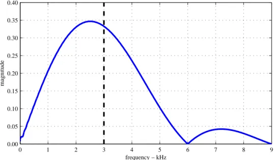
2.4 Frequency content of sinusoidal 3.0kHz pulse signal, obtained using a FFT method. . . 58 2.5 Example of a 3.0kHz sinusoidal continuous signal. . . 61 2.6 Frequency content of 3.0kHz sinusoidal continuous signal obtained
using a FFT. . . 62
2.7 Example of transmitted and received sinusoidal continuous signal
with 3.0kHz. . . 63 2.8 Magnitude curve constituted by a collection of received continuous
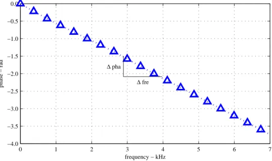
2.9 Phase delay curve constituted by a collection of received continuous signals with different frequencies. . . 65 2.10 Relative position of two sinusoidal continuous signals in the time axis. 66 2.11 Typical oscilloscope displays of two superimposed sinusoidal
contin-uous signals. . . 67 2.12 Example of a sweep signal time history. . . 68 2.13 Frequency content of sweep signal. . . 69 2.14 Example of specific oscilloscope cross-talk noise for an input signal
with an amplitude of 20V and a frequency of 4.0kHz. . . 73 2.15 Example application of cross-talk filtering for pulse signals with
cen-tral frequency of 4.0kHz and amplitudes of 20V, 10V and 5V. . . 75 3.1 Two-dimension body strain. . . 78 3.2 P and S wave propagation, and corresponding directions of particle
oscillation. . . 83 3.3 SV and SH transversal wave types. . . 84 3.4 Wave sources and corresponding wave fronts. . . 85 3.5 P wave multiple reflection inside a solid with finite cross-section. . . . 86 3.6 P wave reflection from a solid-vacuum boundary. . . 87
3.7 Reflected P and S waves amplitude from a incident P wave, at a
solid-vacuum interface. . . 91 3.8 Particle motion of Rayleigh surface wave. . . 93 3.9 Simple cases of pressure distribution along the cross-section of a layer
of fluid in vacuum. . . 93 3.10 Cylindrical axis system. . . 95 3.11 Fundamental modes of wave propagation in a cylinder waveguide. . . 97
3.12 Phase velocity dispersion curves of the 3 first longitudinal modes of
wave propagation. . . 100
3.13 Group velocity dispersion curves of the 3 first longitudinal modes of wave propagation. . . 102
3.14 Phase velocity dispersion curves of the 3 first torsional modes of wave propagation. . . 104
3.15 Group velocity dispersion curves of the 3 first torsional modes of wave propagation. . . 104
3.16 Phase velocity dispersion curves of the 3 first flexural modes of wave propagation. . . 106
3.17 Group velocity dispersion curves of the 3 first flexural modes of wave propagation. . . 106
3.18 Wave source and wave radiation diagram. . . 107
3.19 Ratio between near and far-field wave components. . . 112
3.20 Near-field components velocity. . . 113
3.21 SDOF body vibration scheme. . . 118
3.22 Time history of a SDOF damped free vibration. . . 121
3.23 Steady-state, transient and total responses of a simple mechanical system. . . 123
3.24 Phase difference between load and response of a SDOF system, for different damping coefficients. . . 124
3.25 Magnitude response curves of a SDOF for different damping coefficients.125 3.26 Time history response of damped SDOF system. . . 127
3.27 Magnitude frequency response of a damped harmonic-loaded SDOF system. . . 128
3.28 SDOF system of flexed cantilever. . . 132
4.1 Typical monomer hydrocarbon molecule. . . 143
4.2 Typical polymer molecule. . . 143
4.3 Representation of urethane monomer. . . 145
4.4 Polyurethane main molecular groups. . . 146
4.5 Chemical representation of a simple polyurethane monomer. . . 146
4.6 Polymer chain with covalent bonds between monomers and cross-link bonds, forming an amorphous network skeleton. . . 147
4.7 Simple compression load test on polyurethane cylinder. . . 150
4.8 4 moulds used to prepare the polyurethane rubber samples. . . 154
4.9 Male bender element mould in fixed cap. . . 154
4.10 Estimated wave velocities from bender element testing on one sample over 81 days, determined with different input signals and different signal processing methods. . . 156
4.11 Repeatability of synthetic sample testing with sample age. . . 159
4.12 Repeatability of synthetic sample testing with room temperature. . . 160
5.1 Bender element embedded in triaxial cell cap. . . 167
5.2 Flexural deformation of a bender element tip. . . 168
5.3 Boundary conditions for oscillating bender element. . . 169
5.4 Driving load of a transmitter bender element. . . 170
5.5 Bender element behaviour monitoring set-up, with a laser velocimeter. 174 5.6 Tested UCL-BE and CIS-BE transducers. . . 176
5.7 Illustration of the tested UCL-BE and CIS-BE transducers. . . 176
5.8 UCL-BE’s monitored velocity response and corresponding displace-ment for a harmonic continuous signal. . . 180
5.9 UCL-BE’s monitored velocity response and corresponding displace-ment for a pulse signal. . . 181
5.10 Free UCL-BE’s response function estimate from continuous signal dynamic excitation. . . 182 5.11 Free CIS-BE response function estimate from sweep signal dynamic
excitation. . . 184 5.12 Free UCL-BE’s time responses to pulse signals with various frequencies.186 5.13 Free UCL-BE input and output signals’ frequency content. . . 191 5.14 Free CIS-BE’s time responses to pulse signals with various frequencies.193 5.15 Free CIS-BE input and output signals’ frequency contents. . . 194 5.16 Embedded UCL-BE’s response function estimate from sweep signal
dynamic excitation. . . 195 5.17 Embedded CIS-BE’s response function to sweep signal dynamic
exci-tation. . . 196 5.18 Embedded UCL-BE’s time responses to pulse signals with various
frequencies around the natural frequency. . . 200 5.19 Embedded UCL-BE responses frequency content to pulse signals with
various frequencies. . . 201 5.20 Embedded CIS-BE’s time responses to pulse signals with various
fre-quencies around the natural frequency. . . 203 5.21 Embedded CIS-BE responses frequency content to pulse signals with
various frequencies. . . 204 5.22 Mechanical model of bender element tip embedded in soil. . . 207 5.23 Scheme of multi-step bender element transducers modelling using the
observed properties from the laser velocimeter monitoring . . . 208 5.24 Dynamic displacement amplitudes of UCL-BE and CIS-BE tips. . . . 216 5.25 Pressure exerted by bender element against the embedding medium
5.26 Displacement distribution from flexed bender element tip to lateral
surface along radius. . . 221
5.27 Touching bender elements set-up. . . 223
5.28 Mechanical model of two bender element tips touching, both embed-ded in an elastic medium. . . 224
5.29 Time history and magnitude response of receiving UCL-BE, touching the transmitter, both embedded in a short rubber sample. . . 224
5.30 Response magnitude and phase delay curves of the output signal of the receiving bender element touching the transmitter. . . 225
6.1 Typical bender element test set-up used in the parametric study. . . . 235
6.2 Resonance test of rubber samples set-up, monitored with laser ve-locimeter. . . 240
6.3 Time history and corresponding frequency content of resonant column response of polyurethane rubber sample S22, as monitored by a laser velocimeter. . . 242
6.4 Equivalent shear wave velocities obtained from the torsional and flex-ural resonance frequencies for samples S21, S22, S23 and S24. . . 243
6.5 First flexural and torsional modes of vibration characteristic frequen-cies for sample heights of H = 50mm and H = 76mm and varying diameters. . . 244
6.6 Frequency content of sample S22 - h50 × d50mm partial and total time histories. . . 245
6.7 Wave travel velocity estimates for the repeatability study. . . 248
6.8 Wave travel velocity estimates for the control sample study. . . 250
6.9 Example phase delay curves for samples S15, S22 and S29. . . 252
6.11 Maximum frequency determination for sample S21 - h50 × d38mm using the phase delay and magnitude response curves. . . 255 6.12 Maximum frequency detected at response curves of synthetic rubber
samples. . . 255 6.13 Bender element test system and equivalent mechanical model. . . 257 6.14 Peak features of response magnitude curves of samples S21, S25 and
S29. . . 258 6.15 Peak features of response magnitude curves of samples S29, S30 and
S31. . . 259 6.16 Response magnitude peak features from samples with constant
diam-eter, D = 38mm, and varying heights. . . 260 6.17 Peak features A and characteristic frequency curves of second mode
of flexural vibration, for samples with constant diameter, D = 38mm. 262 6.18 Peak features B and characteristic frequency curves of the third mode
of torsional vibration, for samples with constant diameter, D = 38mm.263 6.19 Peak features C and characteristic frequency curves of the third mode
of flexural vibration, for samples with constant diameter, D = 38mm, and variable heights. . . 264 6.20 Peak features A and C and characteristic frequency curves concerning
samples with constant height, L = 76mm, and variable diameters. . . 265 6.21 Peak features B and characteristic frequency curves concerning
sam-ples with constant height, L = 76mm, and variable diameters. . . 266 6.22 Comparisons between phase delay curves of sweep signals, pi points
and continuous signals for samples S21 and S29. . . 267 6.23 Selection of the frequency range used to determine the group wave
velocity. Obtained from the phase delay and magnitude response curves, for sample S29 - h76 × d38mm. . . 270
6.24 Frequency domain wave velocities for parametric study of rubber sam-ples. . . 272 6.25 Frequency domain normalised wave velocities for parametric study of
rubber samples. . . 273 6.26 Received pulse signals in samples S09, S10 and S11, for an input of
3.0kHz. . . 276 6.27 Received pulse signals in samples S29, S30 and S31, for an input of
3.0kHz. . . 277 6.28 Different travel times estimates for sample S11, for varying input
frequencies. . . 280 6.29 Different travel times estimates for sample S29, for varying input
frequencies. . . 281 6.30 Frequency content of received pulse signals in sample S11 - h20 ×
d75mm, for different frequency inputs. . . 284 6.31 Frequency content of received pulse signals in sample S29 - h76 ×
d38mm, for different frequency inputs. . . 285 6.32 Ratio between signal features E/G for samples S11 and S29 collected
for a range of input signal frequencies. . . 289 6.33 Features E/G ratio in received pulse signal and theoretical near-field
effect. . . 291 6.34 Corrected wave velocity estimates from pulse signals, according to
sample height and diameter. . . 294 6.35 Range of studied sample heights and relative embedment used in the
determination of travel distance. . . 297 6.36 Travel time results using a frequency domain method for the
6.37 Travel time results using time domain method for the parametric study samples. . . 299 6.38 Corrected frequency domain wave velocities. Travel distance
mea-sured between 1.83mm of transducers’ embedded heights. . . 301 6.39 Corrected time domain wave velocities. Travel distance measured
between 0.82mm of transducers’ embedded heights. . . 302 6.40 Wave velocity comparison with slenderness ratio, H/D,for frequency
domain results. . . 305 6.41 Comparison between wave velocity and geometric parameter, H2/D,
for frequency domain results. . . 305 6.42 Wave velocity for frequency domain results, with a travel distance
measured between 60% of the transducer’s embedded height, as cal-culated in section 6.6.1. . . 307 6.43 Sample behaviour model according to geometry parameter H2/D for
frequency domain velocity results. . . 309 6.44 Time domain wave velocities variation with slenderness ratio H/D. . 312 6.45 Time domain wave velocity variation with geometric parameter H2/D.313
6.46 Ratio between the theoretical unbounded near-field effect and total measured dispersion. . . 315 6.47 Direct and reflected travel distances. . . 316 6.48 Study of direct and reflected travel distances ratio variation with
geometry parameters. . . 316 7.1 time history of the received signals for the 1D unbounded and the 2D
bounded numerical modes, extracted from Hardy (2003). . . 327 7.2 representation of finite difference grids of models A and B. . . 334
7.3 pressure distribution on a circular section, subjected to the displace-ment of a node in its centre. . . 336 7.4 time history of received pulse signals at top of the sample, for model
A and model B. . . 338 7.5 reflected wave signal obtained as the difference between the
non-absorbing signal and the non-absorbing signal, for model A. . . 340 7.6 reflected wave signal obtained as the difference between the
non-absorbing signal and the non-absorbing signal, for model B. . . 341 7.7 Wave propagation along the sample’s main axis for model A - h100 ×
d50mm, with non-absorbing lateral surface. . . 347 7.8 Wave propagation along the sample’s main axis for model B - h100 ×
d75mm, with non-absorbent lateral surface. . . 348 7.9 Wave propagation along the sample’s main axis for model B - h100 ×
d75mm, with absorbing lateral surface. . . 349 7.10 Reflected wave components propagating along the sample’s main axis
for model A - h100 × d50mm. . . 350 7.11 Reflected wave components propagating along the sample’s main axis
for model B - h100 × d75mm. . . 351 7.12 representation of generic finite difference model, including
transmit-ting and receiving bender elements. . . 352 7.13 wave velocity for numerical parametric simulation, obtained through
results in the time and frequency domains. . . 355 A.1 Rubber sample geometries used in parametric study. This page may
be used as a pull-out companion to chapter 6. . . 365 B.1 Interpretation Method . . . 367 B.2 Signal Type . . . 368
List of Tables
2.1 Pulse signal travel time estimates from signal features given in figure 2.2. . . 55 3.1 Cylinder waveguide model material properties. . . 101 3.2 Relevant properties of the sample and rigid masses of a resonant
col-umn apparatus according to figure 3.29. . . 138 4.1 Detailed notation of figure 4.10. . . 156 4.2 Wave velocity estimates and deviation from average of each sample
for each of the repeatability tests. . . 157
5.1 Ometron VH300+ LDV properties, given in Image (2000). . . 173
5.2 Description of the two tested bender element transducers. . . 175 5.3 LDV monitoring test summary. . . 177 5.4 Hardware frequency range of the equipment used in the laser
moni-toring of bender element behaviour. . . 178 5.5 Sweep signal properties . . . 181 5.6 Summary of dynamic properties of tested bender elements. . . 206 5.7 Estimated flexural stiffness, static displacements, moment load and
equivalent spring stiffness for UCL-BE and CIS-BE. . . 210 6.1 List of soil properties and triaxial cell bender element test parameters
6.2 Dimensions and reference of rubber samples. . . 234 6.3 Properties of the signals used to excite the transmitting bender
ele-ment during the parametric study. . . 237 6.4 Repeatability study parameters. . . 248 6.5 Control sample study parameters. . . 248 6.6 Control Sample Density. . . 250 6.7 Properties of the Bernoulli-Euler cantilever beam model. . . 261 6.8 Estimated shear-wave velocity using various dynamic methods. . . 272 6.9 Wave velocity estimates from figure 6.27. . . 279 6.10 Travel distances according to different estimates and methods. . . 301 6.11 Velocity variation according to waveguide dispersion frequency limit. 311
7.1 Summary of numerical computer programs used in the analysis of
bender element problems. . . 325
7.2 Properties of the soil medium for numerical models A and B, in
FLAC3D. . . 335 7.3 Small-strain shear stiffness G0 estimation error using first arrival for
numerical models A and B. . . 342 7.4 Properties of the soil medium for second parametric study numerical
models. . . 353
List of Symbols
A area
D diameter
Df dynamic magnification ratio, = a0a/k
Di amplitude of incident compression wave
Dr amplitude of reflected compression wave
E Young’s modulus
EI flexural stiffness
F force
FP far-field compression wave component
FS far-field shear wave component
G shear stiffness
G0 small-strain shear stiffness
H height
I cross-section moment of inertia
IP i mass polar moment of inertia
Jn(x) Bessel function
K bulk modulus
L length
M concentrated mass
N number of monomers in polymer chain
NP near-field compression wave component
NS near-field shear wave component
Rd near-field effect indicative ratio
S seismology term for shear wave
SH horizontally polarised shear wave
SV vertically polarised shear wave
T period, = 1/f
T temperature
T thickness
Ti amplitude of incident shear wave
Tr amplitude of reflected shear wave
Vd characteristic compression wave velocity
Vdf f far-field compression wave velocity, = Vd
Vdnf near-field compression wave velocity
Vs characteristic shear wave velocity
Vf f
s far-field shear wave velocity, = Vs
Vnf
s near-field shear wave velocity
W width
Z(t) amplitude function
∆ dilatation
Γ Kelvin-Christoffel or acoustic tensor
Λ wavelength, = ci/f
β frequency ratio, = ω/ωn
¨
u(t) response acceleration function
˙u(t) response velocity function
η(x) shape function
γij strain
λ Lam´e’s longitudinal elastic constant
µ Lam´e’s transversal elastic constant also known as shear stiffness, = G
∇2 Laplace operator
ω circular frequency, = 2πf
ωD damped free-vibration circular frequency
ωn natural circular frequency
ω harmonic load circular frequency
φ scaler potential function
ψ vector potential function
ρ density τij stress θ angular coordinate ε strain εd compression strain εs shear strain ξ damping ratio
ζ hysteretic dampig ratio
a response amplitude
a0 load amplitude
adi angle of incident compression wave
adr angle of reflected compression wave
ati angle of incident shear wave
atr angle of reflected shear wave
b bond length
c damping coefficient
c∗
generalised damping coefficient
cR velocity of Rayleight surface waves
cc critical damping coefficient, = 2mωn
cd velocity of compression waves in unbounded media, =p(λ + 2µ) /ρ
cg group velocity
ci wave velocity
ct velocity of shear waves in unbounded media, =pµ/ρ
cij elastic constant
d31 piezoelectric strain constant
fD damped natural frequency, = ωD/(2π)
fwd frequency limit for waveguide dispersion
fn natural frequency, = ωn/(2π)
fnf near-field frequency limit, proposed by Arroyo et al. (2003a)
g31 piezoelectric voltage constant
k∗
generalised stiffness
k0 propagation constant in a particular direction
kB Boltzmann constant, = 1.38 × 10⁻²³JK−1
kd longitudinal propagation constant
kt transversal propagation constant
lb embedment length m integer m mass m∗ generalised mass n integer
nP near-field compression wavelength
nS near-field shear wavelength
p(t) load function
p∗
(t) generalised load function
pT(t) harmonic torque load
r radius
t time
td travel distance
u component of displacement
u(t) displacement function
up(t) transient dynamic response
ur component of displacement
ut(t) steady-state dynamic response
uz component of displacement v component of displacement w component of displacement x rectangular coordinate y rectangular coordinate z rectangular coordinate
LDV laser Doppler velocimeter
LVDT linear variable differential transformer MDOF multiple degrees of freedom
RTV room temperature vulcanization
SASW spectral analysis of surface waves
SDOF single degree of freedom
Chapter 1
Introduction
1.1
Prologue
In normal working conditions, most part of the soil mass around a structure is subjected to small strains, less then 0.1%, with higher strains being achieved only locally, (Burland, 1989). Besides, the relationship between strain and stiffness of soils is generally non-linear, (Atkinson, 2000). Only at very small strains does the correlation between strain and stiffness behaves in a linear fashion. It is at these smaller strains that the shear stiffness reaches its maximum value, usually refered to as G0 or Gmax. For this reason it is also known as small-strain shear stiffness. A
characteristic soil strain-stiffness curve is presented in figure 1.1.
When preparing a static or dynamic physical model of a geotechical structure it is relevant to take into account the non-linear behaviour of the soil. It is therefore necessary to obtain, among other properties of the medium, its small-strain shear stiffness, (Arulnathan et al., 2000; Brignoli et al., 1996). Dyvik and Madshus (1985) mentioned the relevance of using G0 in the prediction of soil and soil-structures
be-haviour during earthquakes, explosions, traffic vibration, machine vibration, wind loading and wave loading. In analysis where large strains are considered, the
knowl-10−6 10−5 10−4 10−3 10−2 10−1 100 101 shear strain rate,
stiffness, G
εs%
Figure 1.1: Characteristic strain-stiffness curve of soil’s non-linear behaviour, col-lected from Atkinson (2000).
edge of G0is still relevant since it is one of the defining parameters when considering
the soil’s non-linear behaviour.
Stating the obvious, in order to obtain the small-strain stiffness, soils must be tested at small strains. Despite increasing precision from static test equipment such as local gauges, namely the use of LVDT1, (Brocanelli and Rinaldi, 1998; Cuccovillo
and Coop, 1997; Da-Re et al., 2001), dynamic methods remain the natural option to test at small and very small strain ranges, (Atkinson, 2000).
Bender elements are piezoelectric ceramic instruments used in laboratory geotech-nical dynamic testing. They work as cantilevers which flex or bend when excited by the voltage differential of an electric signal and vice-versa, i.e., they generate a volt-age differential when forced to bend. These transducers are generally used in pairs where one bender element operates as a transmitter and the other as a receiver. The transmitting bender element tip is generally embedded at one end of a soil sample and the receiving bender element tip is, aligned with the transmitter, embedded at
1
the other end. The transmitting bender element transforms the input electric signal into a mechanical motion which disturbs the medium in which it is embedded. This disturbance propagates through the medium in the form of mechanical waves. Some components of these waves reach the other end of the sample where the receiving bender element is at. Wave components with motion transversal to the receiving transducer’s tip are capable of forcing it to bend, and consequently of generating an output electric signal. An example of a pair of bender elements mounted on a triaxial-cell apparatus is presented in figure 1.2
Figure 1.2: Pair of bender elements mounted in a triaxial-cell apparatus.
By comparing the input and output signals, it is presumably possible to obtain the shear wave velocity, which is a characteristic of the medium. The characteristic shear wave velocity can then be used to obtain the shear stiffness of the medium, (Redwood, 1960), as given by:
G0 = ρ · Vs2 (1.1)
where G0 is the small-strain shear stiffness, ρ is the medium’s density and Vs the
Other dynamic methods such as the cross-hole method used in situ, and differ-ent piezoceramic transducers such as shear-plate transducers and compression-plate transducers used in laboratory can also be used to determine wave travel times, (Bodare and Massarsch, 1984; Brignoli et al., 1996). Resonant columns are another laboratory dynamic device used to determine the shear-stiffness and the damping co-efficient of the soil, (ASTM, 1978). Unlike the previous example, resonant columns use the torsional or flexural resonance frequency, rather than a wave velocity, to estimate the medium’s properties, (Stokoe et al., 1994).
Arulnathan et al. (2000) used a mini-hammer in a centrifuge model together with a number of accelerometers to determine the propagation velocity of shear waves in sand. The obtained results were in good agreement with equivalent bender element results obtained for the same medium. AnhDan et al. (2002) have also used accelerometers together with LVDT apparatus to obtain the small-strain stiffness of coarse soils.
In Audisio et al. (1999) and Hope et al. (1999), another example can be found of in situ dynamic testing, known as spectral analysis of surface waves, SASW. Using surface waves, more particularly Rayleigh waves, to test soil as done with the cross-hole method but with no need for bore-cross-holes, makes the SASW testing method less expensive than the cross-hole method, (Nazarian and Stokoe, 1984).
The advantages of using bender elements are that they are relatively cheap and simple to manufacture. They can be used on their own or can easily be integrated into existing and common geotechnical equipment such as triaxial cells, oedometers or direct shear apparatus, (Arroyo et al., 2003a; Thomann and Hryciw, 1990). In this way it is possible to dynamically test soil samples under controlled load conditions, (Viggiani and Atkinson, 1997). They can be used together with other dynamic test apparatus such as the resonant column, as done by Connolly and Kuwano (1999).
bender and an extender, enabling the detection of compression waves as well as of shear waves, as done by Lings and Greening (2001) and later followed by Dano et al.(2003). When testing saturated soils, compression wave are able to propagate at a faster velocity through the relatively incompressible fluid, which might interfere with the detection of the media characteristic compression wave velocity, (Lings and Greening, 2001).
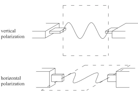
Due to their versatility, bender elements are also used to study the anisotropy of soils. If for the resonant column test one sample per direction needs to be ob-tained to study the anisotropy of a particular material, (M. and Ko, 1994), when using bender elements a pair of these transducers is needed for each chosen direc-tion, while testing a single sample. Placing different pairs of bender elements with different orientations, mounted on the sides of the sample for example, enables the transmission of waves with different polarisations and/or different travel paths, to obtain the different values of the soil’s shear stiffness. Nash et al. (1999) and Joviˇci´c and Coop (1998) in the study of clay, and Belloti et al. (1996), Zeng and Ni (1998) and Kuwano et al. (2000) in the study of sand, for example, have used more than one pair of bender elements in triaxial cell devices in order to study the anisotropy at small-strains of those media. The influence of particle orientation, for example, can be studied in such way, (Lo Presti et al., 1999). Figure 1.3 depicts two pairs of bender elements placed orthogonal to each other and the resulting wave polarisation.
Clayton et al. (2004) also used side-mounted bender elements in a triaxial cell but for different purposes. In this way he was capable of having more than one receiver for a single transmitter, enabling the determination of a more complete picture of the wave propagation properties.
The use of bender elements also carries some disadvantages. Their intrusive nature, when embedded in the soil, means that they disturb the sample near the
Figure 1.3: Study of soil anisotropy with vertical and horizontal bender element placement and consequent wave polarisation.
region where they are placed. Besides, having been originally design to transmit and receive shear wave components, if used in slender samples, and due to the anti-symmetric nature associated with the transmitting bender element flexion, they are expected to excite flexural modes of wave propagation rather than the simpler pure shear waves, (Arroyo and Muir-Wood, 2003). Flexural modes of wave propagation are dispersive in nature, (Redwood, 1960), which may difficult the detection of the actual shear wave velocity, and consequently the estimation of the medium’s shear stiffness.
About the intrusive nature of bender elements, Fioravante (2000) and Fioravante and Capoferri (2001) attempted to use the inertia properties of the transducers by attaching them to the outside of the sample and permitting their free vibration, in air or in fluid but not embedded in the soil, both at transmitting or receiving transversal waves. This variation in the use of bender elements is well suited for the study of anisotropy, since in this type of test multiple pairs of bender elements are usually placed at the sides of the sample. This positioning is difficult to achieve
when the transducers’ tips are embedded in the soil, since they must go through the protective latex membrane, which might jeopardise its impermeability.
Presently, some disagreement remains over the constitutive model of behaviour of a general bender element test system. Also, issues such as the optimum type of signal to excite the transmitting bender element or the best method of signal interpretation are also still not agreed upon. A more traditional behaviour model of bender element systems assumes the mechanical waves to propagate as if in a unbounded medium, similar to a cross-hole test. In this case, there is no dispersion caused by wave reflection and hence no added complexity from this factor. Another constitutive model, considering the geometry of the tested sample and its dynamic modal behaviour, the same as assumed in resonant column tests, is also possible.
The issue of sample geometry is central in this dissertation. Knowing that bars with different geometries have different modal responses, (Clough and Pen-zien, 1993), by establishing a relationship between sample geometry and general dynamic behaviour of the test system, with consequent interference in the obtained results, it is possible to establish this modal behaviour as the most suitable consti-tutive model of bender element testing in general. Besides, if this is accomplished, it is also possible to address the issues of optimum input signal and optimum result interpretation in the context of optimum dynamic response.
1.2
Historical Overview
References to the study of dynamic phenomena such as waves and body vibrations can be traced as far back as Pythagoras in 500 B.C., when he noticed the relationship between the length of vibrating strings and the harmony of the sound they produced. The history of dynamics cannot be separated from the history of physics itself, as well as that of its most influential protagonists. Galileo’s study of the periodicity
of celestial body orbits, Newton’s laws of motion, Euler’s ‘Theory of the Motions of Rigid Bodies’ and Rayleigh’s ‘Theory of Sound’ are but a few distinguished examples. Seismic events are a relevant type of dynamic phenomena. They receive signif-icant attention from the engineering community due to their potential of causing great impacts in human activity. Seismology is a well established field of study, being an important driving force for the development of general dynamic theory. Love’s ‘Some Problems in Geodynamics’ is a noteworthy example. The field of the-oretical seismology is in constant progress, (Aki and Richard, 2002), from which the dynamic testing of soils is but a part.
Burland (1989) and Atkinson (2000), have addressed the notion of non-linear soil stiffness, focussing on the importance of its small-strain behaviour. In this way, greater awareness was obtained for the testing of soils at small-strains, which could mainly be achieved with dynamic testing.
The dynamic testing of soils in situ is traditionally made using the cross-hole method, (Bodare and Massarsch, 1984). A number of sensors are placed in separate boreholes and the records of received shear waves compared. The objective is to de-termine the velocity of the shear wave, which in turn is used to obtain the medium’s shear stiffness. In cross-hole testing the medium is generally assumed to be non-dispersive because of the considerable distance between wave source and receivers, and also because of the considerable distance between wave direct travel path and medium boundaries, (Hoar and Stokoe, 1979), making the estimation of the wave velocity a simpler task.
Laboratory dynamic testing, before the use bender elements, included the use of piezoceramic crystal transducers and resonant columns. In the case of piezocrystals, they too are used to directly measure the velocities of either compression or shear waves, (Brignoli et al., 1996). Resonant columns tests are used according to a different principle. The soil samples are excited, usually in torsion, and the resonance
frequency of the first vibration mode is obtained and used to estimate the medium’s shear stiffness, (Richart et al., 1970). In resonant column testing, the wave dispersion on the soil sample is acknowledged. That is why the first mode of torsional frequency is frequently used, since it is a well known non-dispersive mode of vibration, (Stokoe et al., 1994).
Shirley and Hampton (1978) combined the properties of piezorecamic transduc-ers with the principles of cross-hole testing by using a pair of piezoelectric ceramic plates to transmit and receive mechanical waves. The use of shear wave transducers was not unheard of, (Lawrence, 1963), the merit of Shirley (1978) was the develop-ment of an innovative design for the transducers. Using relatively long thin plates permitted the production and detection of transversal motion through their bend-ing deformation rather than through a shear deformation as done by shear wave transducers. Hence the name bender elements. This slender design significantly re-duces the resonance frequency of the transducers approaching it to the frequencies at which waves propagate in soft soil media without being excessively attenuated. This bending design also permitted a better coupling between the medium and the transducers.
Schultheiss (1981) further developed the design of bender elements, optimising their dimensions so that they could be fitted into oedometers, triaxial cells and sim-ple shear geotechnical apparatuses. Dyvik and Madshus (1985) presented with some detail, a study on bender element performance related with their wiring, concluding that parallel wiring suited the transmitting transducer and series wiring suited the receiver transducer. Dyvik and Madshus (1985) also presented a comparative study between bender element transducers and better established resonant columns, in order to validate their results. The work of Dyvik and Madshus (1985) has become a benchmark in the use of bender elements, and is amongst the most cited works related to this type of testing.
Dyvik and Madshus (1985) and Viggiani and Atkinson (1995) provided generally accepted guidelines in the study of bender element testing. They gave some insight about the issue of wave travel distance as well as having used a frequency domain analysis, in the form of a cross-spectrum between the input and output signal, which they then compared with time domain results.
Joviˇci´c et al. (1996) and Brignoli et al. (1996) presented relevant work, focusing on the phenomena related to bender element testing. Both have explored how best to interpret time domain results and both give relevant consideration to near-field effect as a cause of wave velocity dispersion. Joviˇci´c et al. (1996) also looked at the shape of the input signal and justified the use of an optimised sinusoidal pulse signal. Brignoli et al. (1996) verified the results of bender element tests with those of shear-wave transducers as well as also reflecting on the issue of travel distance.
Blewett et al. (2000) proposed the use of frequency domain technique, just as Viggiani and Atkinson (1995) had. This time using continuous signals with the objective of obtaining the response curves of the system. An interesting comparison between bounded and unbounded sample behaviour was also presented.
Presently, bender elements use has increased despite test standards and generally accepted guidelines not being established yet, (Viggiani and Atkinson, 1997), and the non-agreement about the actual behaviour of the dynamic system. Consequently there is no established method of interpreting the results. There is an ongoing debate about the benefits of using time or frequency domain analysis, pulse or continuous signals, about the relevance of different causes of dispersion, or even about the feasibility of actually obtaining the shear wave velocity using bender elements.
1.3
Strain Level
In normal working conditions most foundation structures cause strains lower than 0.1% to large volumes of the affected ground soil, only locally are higher strains achieved, (Burland, 1989). Besides, soil has a non-linear elastic behaviour where at small strains the stiffness is significantly higher than for larger strains, (Atkinson, 2000). Figure 1.1 ilustrates a characteristic strain level curve.
In situ soil testing, measuring strains above 10−1
%, does not offer the capability of determining soil stiffness at lower strain levels. In terms of laboratory testing, static methods such as local gauges have a limited precision that does not allow them to measure strains lower than 10−3
% for which a maximum stiffness can generally be obtained. Dynamic laboratory testing is then left as the single option to obtain measurements for the lowest strains, ǫ < 10−2
%, of which bender elements are a suitable example, (Joviˇci´c and Coop, 1997).
In terms of the shear strain levels involved in the use of bender elements, Dyvik and Madshus (1985) estimated the transmitting transducer to be in the range of ǫ ≈ 10−3
%. Leong et al. (2005) estimated the strain level of the receiving bender element to be in the range of ǫ ≈ 10−4
%, when touching the transmitting bender element. There is another estimate of strain level in the range of ǫ ≈ 10−4
%, given by Pennington (1999).
1.4
Monitoring of Bender Element Behaviour
When testing with bender elements, the transmitted and received electric signals are used to characterise the system. When doing so, it is inherently assumed that the transducers have a mechanical motion with a time history equivalent to the corre-sponding input signal that forced their movement. This assumption is questionable since the bender elements have non-zero mass and non-zero stiffness, then they must
behave, mechanically, as a Newtonian system, where the effect of inertia is present. If, for example, the body of the bender element is fixed to a cap and its tip free to move, these are common boundary conditions usually described as those of a cantilever. Clough and Penzien (1993) explain how the dynamic bending or flexural motion of a cantilever can be analytically modelled as a single degree of freedom system, SDOF, (section 3.10). The response of a generic SDOF to a harmonic excitation is presented in section 3.8.5, and illustrated in figures 3.25 and 3.24. For an excitation force of constant magnitude, the magnitude of the response varies with frequency, (equation 3.84). Also, there is a phase difference between the excitation and the response which also varies with the excitation frequency and can be as much as 180o, (equation 3.84). The observation that such a system can vibrate not in phase
with the excitation force is well known in mechanical dynamics, but somehow not generally assumed when dealing with the behaviour of bender elements.
In order to better understand the behaviour of bender elements, some authors have monitored it. Shirley (1978) mentions the resonance frequency of the bender elements used, but does not mention the method to obtain such a value. The earliest reference about the monitoring of bender elements is given by Schultheiss (1982). The method consisted of wiring the piezoelectric ceramic to two independent electric circuits. One circuit is used to excite the transducer in the normal way and the other to transfer its response back to an electric signal. This method of monitoring initially appears to be quite ingenious, yet the results show a response which is perfectly faithful to the excitation, thus not plausible. Such a result can be explained by an electric leakage, where the exciting electric signal reaches the wiring circuit responsible for the response monitoring directly. Since the received signal corresponding to the actual mechanical bending of the transducer would have a significantly lower amplitude than that of the input signal; if an electric short-circuit does occur, it would dominate the received signal. One other possibility is
for the input signal to be harmonic with a frequency comparatively lower than the resonance frequency of the transducer, allowing a steady state response with barely no phase delay, (Clough and Penzien, 1993).
Schultheiss (1982) used the same self monitoring method proposed by Shirley (1978), and for two pulse signals with different frequencies obtained two distinct responses. For a lower frequency of 2.96kHz the transducer is observed to emulate the excitation signal perfectly. At a higher frequency of 29.6kHz, the transducer has shown again to emulate the excitation signal but now with some discontinuities in the response trace. This second behaviour, namely the observed discontinuities, was called overshooting.
Brocanelli and Rinaldi (1998) used an accelerometer to monitor the response of the bottom plate to which the transmitting bender element is mounted and fixed. Hitting the bottom plate and inducing a pulse load and then exciting the bender el-ement with a sinusoidal signal enabled the determination of the magnitude response curve of the composed system. Such data allowed to distinguish and identify the individual resonance frequencies of both the bender element and the plate. Nev-ertheless, since the behaviour of the plate is dominant, the results concerning the bender element are less reliable.
Greening and Nash (2004) have monitored the behaviour of a transmitting ben-der element by placing a strain gauge in direct contact with the piezolectric ceramic plate and encapsulating them together in epoxy resin. Using a random signal, the response magnitude and phase delay curves were obtained for a comprehensive range of frequencies. The obtained curves are characteristic of a simple mechanical de-vice, indicating a magnitude peak and phase shift of equal frequency, believed to be the resonance frequency of the bender element. See section 3.8.5 for details about similar response curves.
step was to make a receiver bender element touch the transmitter and monitor it, (Lee and Santamarina, 2005; Leong et al., 2005). The problem with this method is that the monitoring data is the signal from the receiver bender element. So, the receiving transducer is the one being directly monitored and not the transmitter. The application of this method requires the assumption of a perfect coupling between the tips of a pair of bender elements with the same electric wiring, series or parallel. In normal testing, it is not possible to verify such boundary condition. Besides, bender elements are used to excite and be excited by the soil through their much larger lateral surfaces, and not just by their tip end.
By making the receiver bender element touch the transmitter bender element, the dynamic behaviour of one transducer is influenced by the other. What is then actually being studied is this composed system and not the independent behaviour of one of the transducers. Neither Lee and Santamarina (2005) nor Leong et al. (2005) thoroughly describe the test system and it is taken into account, when associating the obtained results with the transducers’ properties. Nevertheless, it is possible to compare the transmitted and received signals and estimate how faithfully the bender elements react to the transmitted signal. Leong et al. (2005) found no significant time delay between the transmitted and received signals. These were similar but not the same, making clear that the received signal has a different time history than that of the transmitted signal, with a different frequency and shape; particularly after the transmitted signal has ended. the received signal indicates some further movement from the transducers, as would be caused by inertia effects.
Lee and Santamarina (2005) mention another method of monitoring a bender element transducer which is quite simple. A single bender element tip is left free to vibrate, excited by an instantaneous impact and its response recorded, especially its resonance frequency. In this work, the result were compared with an analytical model allowing their association with the flexural stiffness of an equivalent beam,
and consequently, the calculation of the Young modulus stiffness constant.
Arulnathan et al. (1998) conducted numerical work where the propagation of waves in an elastic two dimensional medium is studied. The mechanical behaviour of the transmitting and receiving bender elements was also considered in the model and so their behaviour could be studied. A varying time delay between the applied force and the tip displacement was detected and estimated between 3.0% and 8.5% of the input signal period. No correlation was proposed between the observed time delay and the phase delay that occurs in simple mechanical systems, and which also varies with excitation frequency, (section 3.8.5). Therefore it is not possible to determine how faithfully the numerical result comply with such particular theoretical behaviour. It would also be interesting to compare the behaviour of the bender element, and the surrounding soil, but such results were not presented.
1.5
Travel Distance
Concerning the travel time and travel distance, necessary to calculate the wave velocity in bender element testing, the determination of travel distance is generally considered the less problematic of the two. Although related with the introduction of the use of bender elements, Shirley and Hampton (1978) did not elaborate on the subject of travel distance, simply referring to it as the distance between the transducers. Dyvik and Madshus (1985), followed by Brignoli et al. (1996) and Viggiani and Atkinson (1995) have proposed and justified the measurement of travel distance as the minimum distance between transducer tips, also known as tip-to-tip distance. The tip-to-tip-to-tip-to-tip travel distance is commonly assumed by a variety of authors, for instance Kuwano et al. (1999), Dano and Hicher (2002), Kawaguchi et al. (2001) or Pennington et al. (2001), with or without explicit justification.
Dyvik and Madshus (1985) compared the dynamic results from three different clay samples, using the resonant column and bender element tests. They observed that the results from the bender element test fitted best the resonant column re-sults for travel distances measured tip-to-tip. An analysis of those same rere-sults can indicate that the effective travel distance for higher soil stiffness, if all other things remain equal, would in fact be even smaller than the tip-to-tip distance. The bender element tests were conducted using a square pulse signal associated with significant uncertainty in the interpretation of results, (Joviˇci´c et al., 1996), which must extend to the proposed conclusion of correct wave travel distance.
Viggiani and Atkinson (1995) used bender elements to test 3 samples with differ-ent heights, between 35mm and 85mm. For each sample, three travel time estimates were obtained for different stress states using square and sinusoidal pulse signals. The chosen linear relationship between the results from different samples, at similar stress states, indicate the correct travel distance to be the tip-to-tip distance. Brig-noli et al. (1996) also came to the conclusion that the correct travel distance must be measured between tip-to-tip. Samples with different heights were tested with bender elements as well as with shear-plates which support his conclusion. Brignoli et al. (1996) used an alternative reference to sample and embedment heights by using the relative embedment heights of the transducers in relation to that of the samples. The two cases referred to were for relative embedment heights of 3% and 14%.
Alternatives to the tip-to-tip travel distance are not commonly proposed. Fam and Santamarina (1995) used the distance between mid-embedded height but did not justify it.
When dealing with direct wave travel times and imagining the wave first arrival, it seems intuitive to picture the receiver being first excited at its tip end. If the same principle is applied to the transmitter, even though it is forced to move as
a single body, again it is easy to picture the disturbance caused by the tip end to propagate ahead of other wave components. If, on the other hand, all the signal content is considered, and not just its first arrival, then both the transmitting and receiving transducers are fully engaged in a mechanical sense. One could suggest for the travel distance to be measured between the centres of applied and received pressure. Also, since the estimation of travel time is itself problematic, it cannot be used to undoubtedly verify the travel distance.
1.6
Scope of Thesis
Chapter 2 describes the different signals used to excite the transmitting bender ele-ment. Each type of transmitted signal and consequent received signal are commonly associated with a particular method of interpreting the results. These methods are also explained.
Chapter 3 presents the relevant theoretical background used to support the in-terpretations made of the bender element related phenomena. Wave propagation theory, body vibration theory, wave radiation and dispersion are some of the sub-jects referred to.
Chapter 4 explains the use of synthetic rubber as a replacement for soft soil samples. The properties of polyurethane rubber are explained and compared to those of soft soils.
In chapter 5 the dynamic properties of bender element transducers are studied in detail. The results from an independent monitoring of their behaviour is carried out and the results compared with simple numerical and analytical models.
Chapter 6 presents the results from the geometry parametric study. The sample geometry is related with the differences in results, according to established theory of body motion and wave propagation.
In chapter 7 the bender element and soil sample test system is modelled using specific numerical tools. Again the geometry of the sample is varied in order to establish a relationship with its dynamic behaviour.
Chapter 8 contains the relevant conclusions made from the observation of the presented results and consideration of relevant theoretic background.
Chapter 2
Signal Properties and Processing
Methods
In this section, different types of input signals used when testing with bender ele-ments are explained. These are electric signals which excite the piezoelectric ceramic plate by applying a voltage differential, forcing it to flex or bend. The electric sig-nals are generated and transmitted by a function generator or similar device. Both a function generator and a personal computer, more specifically its sound card, are used henceforward.
There are a number of different methods of signal processing available, each permitting, in principle, the estimation of the desired wave velocity. A clear distinc-tion between these methods can be placed at the domain in which the results are processed, time domain or frequency domain.
2.1
Pulse Signal
The impulse or pulse signal is a type of signal commonly used in dynamic testing. This type of signal has been employed since the beginning of testing with bender elements, (Shirley, 1978). It is possible to interpret pulse signal results in the
fre-quency domain, as done by Mancuso et al. (1989), for cross-hole test results for example. Still, pulse signals offer an intuitive interpretation of results in the time domain. The wave travel time can be measured directly in a graphic representation of the transmitted and received signals’ time histories, (figure 2.2).
A well known dynamic geotechnical test, the cross-hole method, (Bodare and Massarsch, 1984; Hoar and Stokoe, 1979), uses the same method of wave travel time estimation, serving as a theoretical basis for its use in bender element testing. The cross-hole test method also uses impulse loads, and the response is measured at one or more points positioned away from the source. Even though the bender element and cross-hole test methods have similarities, especially when pulse signals are used to obtain results in the time domain, there are obvious differences between the two. Such differences relate to the boundary conditions and properties of the input signal. Bender elements are most used in somewhat small samples of relatively soft soil where the amplitude of the initial disturbance is small, with strains in the range of ε ∈ [10−3
10−5
]%, (Dyvik and Madshus, 1985). In the cross-hole method the transducers are placed much further apart and the impulse loads created by a significant impact of some kind. So, not only the dimensions and geometry of the media in which the waves propagate are significantly different, but in the cross-hole method the properties of the transmitted signals are limited due to their impact nature.
Because of the established use of the cross-hole test method, testing with bender elements ‘inherited’ some of the assumptions concerning the dynamic behaviour of the wave propagation. One such assumption is the consideration of unbounded wave propagations in bender element testing as for the cross-hole method, (Bodare and Massarsch, 1984). In this way the influence of the sample boundaries is disregarded. Such assumption of unbounded wave propagation is challenged with the results presented in chapter 6.
Pulse signals are characterised by their finite duration, implicit in their name. This finite nature of the pulse signals in the time domain means that the dynamic phenomena related with the consequent body vibration and wave propagation are transient, (Clough and Penzien, 1993). The relationship between transient and steady-state body responses, and specific benefits of each for testing with bender elements, is explored in theoretical terms in section 3.8 and in practical terms in chapter 5.
One property of the pulse signal is its shape or form. In figures 2.1(a) and 2.1(b) are represented two typical shapes of pulse signals, one sinusoidal and an-other square, commonly used in bender element testing, (Dyvik and Madshus, 1985; Pennington, 1999). time voltage (a) sinusoidal time voltage (b) square
Figure 2.1: Sinusoidal and square pulse signals representation.
It became a matter of some discussion which of the two shapes of pulse signal, sinusoidal or square, is more appropriate for bender elements testing. The square pulse signal, (figure 2.1(b)), as used by Bates (1989), Viggiani and Atkinson (1995) or Shibuya et al. (1997) for example, has a very well defined start but no other noticeable features. The start of the square signal is point from which the travel time is measured, Joviˇci´c et al. (1996). Square signals resemble the impact loads
used in the cross-hole test method, (Bodare and Massarsch, 1984), as does the direct time domain method used to estimate the wave travel time. A mathematical representation of a square pulse signal is given,
y(t) = a for t0 ≤ t ≤ (t0+ T )
y(t) = 0 for t < t0 and t > t0+ T
(2.1)
where a is the amplitude, t is the time, T is the period of the signal and y(t) its magnitude.
Problems concerning the use of square pulse signals are related to its sharp initial rise. An instantaneous variation can be expressed analytically as done in equation 2.1 and even reproduced as an electric signal by a digital function generator. But, mechanic devices with finite mass and stiffness, also known as Newtonian systems, cannot respond in such manner. Due to the presence of inertia forces it is not possible to obtain instantaneous variations in motions, equivalent to infinite accelerations. Therefore, when using square signals a discrepancy between the input signal and the actual movement of the transducer must be expected. Consequently, the correlation between the input signal and the transducer’s motion is not straightforward and neither is the overall correlation between the input and output signals.
Due to their instantaneous variation in the time domain, square pulse signals have a very broad frequency content with no particular main or central frequency. This means that frequency dependent dispersion phenomena, such as the near-field effect, explained in section 3.6, and modal wave propagation, explained in section 3.2, cannot be avoided. This is another reason why the use of square pulse signals has gradually become less common in bender element testing, where the boundary conditions of the test system are more prone to the mentioned dispersive phenomena, (Arroyo, 2001; Joviˇci´c et al., 1996).
Sinusoidal pulse signals, as the one represented in figure 2.1(a), are also com-monly used in bender element testing. Examples can be found in Brignoli et al. (1996) or Fioravante (2000). This type of pulse signal is defined,
y(t) = a sin(ωt + θ) − a sin(θ) for t0 ≤ t ≤ t0+ T
y(t) = 0 for t < t0 and t > t0+ T
(2.2)
where a is the amplitude, ω is the pseudo-frequency, given by ω = 1/(2πT ), and θ is the phase origin. Generally, the phase step is set at 0o, as in figure 2.1(a), but other
values can also be used, (figure 2.3). The frequency of the signal is referred to as a pseudo-frequency because it is not he actual frequency of the signal, serving only as a reference. The sinusoidal pulse signal does not follow a Dirac function, with a single frequency, having instead a broad frequency content, accounting for he signal initial and final accelerations.
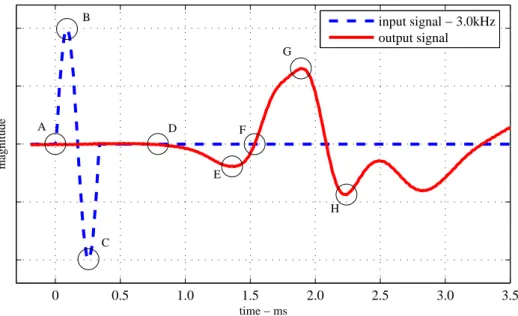
When using a pulse signal to excite the transmitting transducer, the time his-tories of the transmitted and received signals are used to obtain directly the wave travel time. An example of a transmitted and received pulse signal is given in figure 2.2. The input sinusoidal pulse signal has a phase of 0o hence the equilibrium. This
example is similar to several other results from similar test set-ups and clay mate-rials, (Hardy et al., 2002). The travel time can be measured in the horizontal time axis between two characteristic points of the input and output curves.
In figure 2.2 some characteristic features of the transmitted and received signal curves are marked. From these a number of travel time estimates can be obtained. Features A, B and C mark the start, the first local maximum and the first local minimum of the transmitted signal. On the received signal the characteristic features marked are D - first deflection, E - first local minimum, F - first through zero, G - first maximum and H - second local minimum. Assuming that features in the transmitted
0 0.5 1.0 1.5 2.0 2.5 3.0 3.5 time − ms magnitude input signal − 3.0kHz output signal A B C D E F G H
Figure 2.2: Transmitted sinusoidal pulse signal and correspondent received signal time histories, and relevant signal features for travel time estimation.
signal are related with features in the received signal, the time difference between such features gives the desired wave travel time. Table 2.1 presents the travel time estimates obtained using the time differences between the mentioned points which might possibly be related.
Peak Features Travel Time
A-D 0.76ms
A-E 1.36ms
A-F 1.54ms
B-G 1.81ms
C-H 1.98ms
Table 2.1: Pulse signal travel time estimates from signal features given in figure 2.2.
It is clear, just by looking at the input and output curves, that the received signal is a distorted version of the transmitted signal. Plausible sources for the observed signal distortion are wave dispersion and particular mechanical response