A multimodal approach to distinguish MCI-C from MCI-NC subjects

FACULDADE DE CIˆENCIAS

DEPARTAMENTO DE F´ISICA

A multimodal approach to distinguish

MCI-C from MCI-NC subjects

Rochelle Ann Costa Silva

Mestrado Integrado em Engenharia Biom´edica e Biof´ısica

Perfil em Sinais e Imagens M´edicas

Disserta¸c˜ao orientada por:

Orientador Externo: Professora Dra. Margarida Silveira, Instituto de Sistemas e Rob´otica (ISR), Instiuto Superior T´ecnico (IST)

Orientador Interno: Professor Dr. Nuno Matela, Instituto de Biof´ısica e Engenharia Biom´edica (IBEB), Faculdade de Ciˆencias da Universidade de Lisboa

(FCUL)

First of all, I would like to express my very special thanks to Prof. Dr. Margarida Silveira, from Instituto Superior T´ecnico (IST), for having accepted to be my supervisor for this thesis in Institute for Systems and Robotics (ISR), in Lisbon. I am very grateful for having had the opportunity and privilege to learn and achieve success in one of the most important experience of my academic life. I truly value all her guidance, support, patience in helping to solve the technical problems that occurred, and the knowledge transmitted throughout the development of the present thesis. I also acknowledge all the corrections and comments on this written work, which were fundamental.

I would also like to express my deep gratitude to Dr. Jonathan Young from Centre for Neuroimaging Sciences, King’s College London, for responding very promptly to my e-mails and clearly explaining the key steps to implement the method from his article. I also thank Prof. Dr. Nuno Matela, for having promptly accepted to be my internal supervisor, for being accessible to help me when needed, and for the comments and suggestions on this written work.

My gratitude also goes to Prof. Dr. Eduardo Ducla Soares for presenting the wonderful world of Biomedical Engineering in my 12th grade and to Dr. Maria Jo˜ao Rosa and Dr. Janaina Mour˜ao Miranda with whom I did an internship in London in my third year of the course. They were instrumental in my choice of specialising in such an interesting area which is Machine Learning.

I appreciate all the support and advice provided by my friends, which helped me over-come stressful moments, and thank them for the great memorable times spent together, during these 5 years of my academic life.

Finally, to my beloved parents I thank their love, trust, patience and motivation. A special thank you to my brother Ryan, who has always been there for me at all times.

Alzheimer’s Disease (AD) is one of the most common neurodegenerative diseases, affect-ing 60-80% from all dementia cases. Unfortunately, the cure for AD is still not known and only some treatments can be done in its early stages to slow up the symptoms and cognitive decline, avoiding worst patients’ living conditions. As most of the AD diagnoses are late, it increases the difficulty of applying the strategies and treatments available. Therefore, current studies aim at detecting AD at an early stage. For this purpose, they are studying mild cognitive impairment (MCI) subjects, as this is normally the first condition before developing AD. Nonetheless, not all MCI patients convert to AD, some remain stable or even may reverse the cognitive decline. In this sense, being able to dis-tinguish between MCI-converters (MCI-C) and MCI-non converters (MCI-NC) reveals a quite important task.

In order to distinguish between these and other groups of subjects many classifiers can be used. Classifiers are machine learning algorithms which apply artificial intelligence. These are extremely useful to identify patterns in, for example, medical brain images, to find disease related patterns and try to achieve an early and reliable diagnosis. The Support Vector Machine (SVM) is a widely used classifier for AD studies and is very appealing as it deals well with high-dimensional problems, which is present when using neuroimages because of the high number of voxels in each image. Nonetheless, SVM is a non-probabilistic classifier and only provides the class predicted for a given test. In a clinical perspective, it would be advantageous to also have a confidence level about the prediction made, to avoid diagnosis being hampered by overconfidence. Hence, of late the interest in probabilistic classifiers is rising. The Logistic Regression (LR) and the Gaussian Process (GP) are examples of probabilistic classifiers, but few studies used these methods to present results for AD classification, additionally the analysis of the posterior probability given by these classifiers is also still not well explored.

In this context, this thesis proposes the comparison of the performance of probabilistic (LR and GP) and non-probabilistic (SVM) classifiers for AD context with special in-terest in reaching good results for MCI-C vs MCI-NC. These tests were done using two neuroimaging modalities: the deoxyglucose Positron Emission Tomography (FDG-PET) and structural Magnetic Resonance Imaging (sMRI), in single modal and multimodal approach. A whole-brain approach was chosen, to avoid restringing the model just for certain brain regions. For feature selection methods, the LASSO and group LASSO with L1/L2 regularization, for both single and multimodality cases, were used respectively.

Four different binary classification tests involving AD, MCI and elderly cognitive normal (CN) subjects from the Alzheimer’s Disease Neuroimaging Initiative (ADNI) database,

were performed: AD vs CN, AD vs MCI, CN vs MCI and MCI-C vs MCI-NC with a con-version period of 24 months. The results demonstrated the advantage of using GP and LR as they can achieve state-of-the art classification results and be better than SVM, in most cases, while providing posterior probabilities that will help evaluate how confident the classifier is on its predictions. However, to distinguish MCI-C and MCI-NC, SVM seemed to get better results, with LR being just a little worse than SVM. The poste-rior probabilities from GP attracted more attention, because they demonstrated higher confidence in results, whereas LR posterior probabilities were mostly near the thresh-old value, meaning that the class is not chosen with a lot of confidence. Although the multimodal approach did not show always the best results, for the MCI-C vs MCI-NC classification it outperformed the single modality results, independently of the classifier used. Thus, exhibits that is useful to joint information of different modalities to help distinguish between MCI-C and MCI-NC.

Keywords

Alzheimer disease (AD), Mild cognitive impairment (MCI), classification, feature selec-tion, posterior probability

A Doen¸ca de Alzheimer (AD, do inglˆes Alzheimer’s Disease) ´e uma doen¸ca neurodege-nerativa com crescente prevalˆencia que afecta pessoas com idade mais avan¸cada, habi-tualmente superior a 65 anos, e constitui entre 60-80% de todos os casos de demˆencia. Provoca uma progressiva degrada¸c˜ao dos neur´onios e disfun¸c˜ao das sinapses, que cons-tituem a regi˜ao de liga¸c˜ao entre neur´onios. Acredita-se que estas altera¸c˜oes sejam con-sequentes da acumula¸c˜ao de placas da prote´ına beta-amyloide no meio extracelular e de altera¸c˜oes anormais na prote´ına tau no meio intracelular. Consequentemente, com a progress˜ao da doen¸ca, o doente come¸ca a manifestar perda de mem´oria, dificuldade em formular pensamentos e altera¸c˜oes do comportamento, chegando a um estado em que se repercute nas atividades da vida di´aria. Atualmente, n˜ao existe cura para a AD, apenas alguns tratamentos que podem ser feitos para tentar retardar os sintomas e o decl´ınio cognitivo. Estes conseguem ser mais eficazes nas primeiras fases da doen¸ca evitando assim piores condi¸c˜oes de vida para os doentes. Como geralmente o diagn´ostico da AD ´

e tardio, a efic´acia dos tratamentos dispon´ıveis torna-se ainda mais limitada. Neste con-texto, a doen¸ca de Alzheimer ´e vista como um problema de sa´ude p´ublica com elevado impacto econ´omico, tendo sido identificada como uma prioridade na investiga¸c˜ao atual. Muitos estudos tˆem como principal objetivo a dete¸c˜ao precoce da AD, para que os tratamentos possam ser usados com a devida antecedˆencia, sendo mais ben´eficos para o doente. Neste sentido, existe interesse no estudo do d´efice cognitivo ligeiro (MCI, do inglˆes: Mild Cognitive Impairment ), visto que ´e considerado como um estado prodr´omico da doen¸ca de Alzheimer, ou seja, doentes com MCI apresentam sintomas que podem indicar o in´ıcio de AD antes que os sintomas mais espec´ıficos da doen¸ca surjam. No entanto, nem todos os casos de MCI desenvolvem AD, alguns permanecem est´aveis ou podem reverter o decl´ınio cognitivo. Deste modo, tem especial importˆancia con-seguir distinguir sujeitos com MCI que poder˜ao converter (MCI-C), num determinado espa¸co de tempo, dos que n˜ao ir˜ao desenvolver a doen¸ca, ou seja, os MCI n˜ao conver-sores (MCI-NC). Diversos m´etodos de aprendizagem autom´atica que aplicam algoritmos de inteligˆencia artificial tˆem sido utilizados para reconhecer padr˜oes nos dados obtidos atrav´es de t´ecnicas ou exames m´edicos. Pretende-se encontrar padr˜oes nos dados rela-cionados com a doen¸ca e alcan¸car um diagn´ostico precoce confi´avel, atrav´es de classi-fica¸c˜oes com elevada precis˜ao obtidas por estes algoritmos. A combina¸c˜ao dos dados m´edicos com a inteligˆencia artificial deu origem a uma tecnologia interdisciplinar, a que se d´a o nome de diagn´ostico auxiliado por computador (CAD, do inglˆes: Computer-Aided Diagnosis). Nos exerc´ıcios de CAD, em particular quando se usam t´ecnicas de neuroimagem, para a cria¸c˜ao um modelo de classifica¸c˜ao s˜ao definidas normalmente cinco etapas: o pr´e-processamento das imagens, a extra¸c˜ao de caracter´ısticas, a sele¸c˜ao

de caracter´ısticas, a classifica¸c˜ao e a finalmente avalia¸c˜ao do desempenho do classifi-cador. O pr´e-processamento pode envolver v´arias fases, sendo essencialmente usado para eliminar a presen¸ca de ru´ıdo e heterogeneidades e fazer o alinhamento das imagens. Tanto a extrac¸c˜ao como a sele¸c˜ao das caracter´ısticas permitem reduzir o problema da elevada dimensionalidade existente nas neuroimagens, que adv´em do excessivo n´umero de voxels/caracter´ısticas presentes em cada imagem.

Os exames m´edicos dispon´ıveis para facilitar o diagnostico da AD s˜ao diversos e incluem exames de neuroimagem, an´alises laboratoriais, testes gen´eticos e neurofisiol´ogicos. Neste trabalho, foram usadas duas modalidades de imagem que em estudos anteriores provaram ser vantajosas para o diagnostico da AD: a Tomografia por Emiss˜ao de Positr˜oes 8 F-Fluorodesoxiglucose (FDG-PET, do inglˆes: fluorodeoxyglucose Positron Emission To-mography) que permite detetar hipometabolismo nas regi˜oes afetadas pela doen¸ca, e as imagens estruturais de Ressonˆancia Magn´etica (sMRI, do inglˆes structural Magnetic Res-onance Imaging) que permitem detetar perda de volume do tecido cerebral. Ao juntar a informa¸c˜ao destas duas modalidades, ´e poss´ıvel fornecer ao classificador diferentes tipos de informa¸c˜ao, funcional e estrutural, podendo alcan¸car previs˜oes mais precisas. Por conseguinte, estas t´ecnicas foram testadas individualmente, mas tamb´em numa abor-dagem multimodal.

Para evitar o elevado n´umero de voxels/caracter´ısticas presentes nas imagens, deter-minados estudos usam apenas certas regi˜oes do c´erebro. No entanto, foi preferida a abordagem em que todos os voxels/caracter´ısticas do c´erebro s˜ao usados para n˜ao limi-tar o estudo apenas a determinadas zonas. Para selecionar as regi˜oes mais relevantes de todo o c´erebro e diminuir o problema da dimensionalidade foram usados dois m´etodos de sele¸c˜ao de caracter´ısticas: o LASSO, para o caso em que se usou cada modalidade individualmente, e o group LASSO multi-task, no caso multimodal.

O classificador mais utilizado para estudos de AD ´e a m´aquina de vetores de suporte (SVM, do inglˆes: Support Vector Machine). Este classificador ´e apelativo por se adequar a problemas de elevada dimensionalidade e apresentar bons resultados. No entanto, SVM ´

e um classificador n˜ao-probabil´ıstico, ou seja, devolve apenas a classe que prevˆe para um determinado teste e n˜ao uma probabilidade associada. Numa perspectiva cl´ınica, seria mais vantajoso ter uma medida de confian¸ca quanto `a previs˜ao feita pelo classificador. Recentemente, foram introduzidos dois classificadores que devolvem probabilidades `a posteriori: o Processo Gaussiano (GP, do inglˆes Gaussian Process) e a Regress˜ao log´ıstica (LR, do inglˆes Logistic Regression). Por´em, ainda n˜ao foram muito explorados em estudos de AD, especialmente em rela¸c˜ao `as suas probabilidades `a posteriori.

Neste ˆambito, com a presente tese testaram-se trˆes classificadores (SVM, GP e LR), numa perspectiva multimodal, que junta dados FDG-PET e sMRI da base de dados

Alzheimer’s Disease Neuroimaging Initiative (ADNI), bem como numa abordagem usan-do as modalidades individualmente. Estes classificausan-dores foram utilizausan-dos em quatro testes de classifica¸c˜ao diferentes, nomeadamente, para distinguir: AD de sujeitos com idades avan¸cadas e cogni¸c˜ao normal (CN); AD de MCI; CN de MCI e com maior inte-resse os MCI-C de MCI-NC, num per´ıodo de tempo de convers˜ao 24 meses. A partir dos resultados obtidos foi poss´ıvel verificar que tanto o GP como o LR apresentaram resul-tados de classifica¸c˜ao melhores que o SVM, para os casos AD vs CN, AD vs MCI e CN vs MCI. No entanto, na classifica¸c˜ao verdadeiramente pertinente em termos cient´ıficos, ou seja, quando se testou MCI-C vs MCI-NC, o SVM revelou melhores resultados, sendo que o LR n˜ao ficou muito abaixo do SVM, j´a o GP teve uma performance inferior. ´E importante salientar que o GP apresentou vantagens em rela¸c˜ao `as probabilidades `a posteriori exibidas pelo LR, visto que demonstrou mais confian¸ca nas previs˜oes feitas, enquanto o LR apresentou probabilidades `a posteriori mais pr´oximas do limiar entre a escolha de pertencer a uma classe ou outra. Com esta diferen¸ca foi poss´ıvel demostrar a relevˆancia de ter em considera¸c˜ao a an´alise das probabilidades `a posteriori, em vez de se limitar `a analise da precis˜ao do classificador. Em rela¸c˜ao ao n´umero de caracter´ısticas usadas, o LR necessitou um maior n´umero em compara¸c˜ao ao GP ou SVM, apesar disso, n˜ao revelou ter um custo computacional superior aos outros dois classificadores. Quanto aos m´etodos de sele¸c˜ao de caracter´ısticas, LASSO e group LASSO multi-task, destaca-se que ambos foram eficientes em diminuir o n´umero de caracter´ısticas e selecionaram regi˜oes pertinentes, como o hipocampo, amigdala, t´alamo, putamen e ventr´ıculo lateral, que est˜ao de acordo com as regi˜oes detectadas em estudos anteriores. Em alguns ca-sos, a abordagem multimodal n˜ao revelou ser superior aos resultados obtidos usando as modalidades individualmente. N˜ao obstante, para a distin¸c˜ao entre C vs MCI-NC, independentemente do classificador usado, os resultados foram melhores aos obtidos quando se usou as modalidades individualmente. Assim demonstra-se que uma abor-dagem multimodal apresenta vantagens para diferenciar estes dois grupos de sujeitos.

Palavras Chave

Doen¸ca de Alzheimer, D´efice cognitivo ligeiro, classificadores, selec¸c˜ao de caracter´ısticas, probabilidade `a poteriori

Acknowledgements iv

Abstract vi

Resumo viii

List of Figures xiii

List of Tables xv

Acronyms xvi

Symbols xviii

1 Introduction 1

1.1 Alzheimer’s Disease . . . 2

1.2 Motivation and problem identification . . . 6

1.3 Use of machine learning for early diagnosis . . . 7

1.4 Contribution of Thesis and Thesis Outline . . . 12

2 State-of-the-art 14 2.1 Multimodality. . . 18 2.2 Feature Selection . . . 20 2.3 Classifiers . . . 21 3 Proposed Methods 24 3.1 Feature Selection . . . 24

3.1.1 LASSO with L1 penalty . . . 24

3.1.2 Group LASSO multi-task with L1/L2 penalty . . . 25

3.2 Classifiers . . . 27

3.2.1 SVM . . . 27

3.2.1.1 Kernel Trick . . . 31

3.2.1.2 Nested Cross-validation to discover C parameter . . . 31

3.2.2 Logistic Regression . . . 33

3.2.3 Gaussian Process . . . 34

3.2.3.1 Bayesian theory . . . 34

3.2.3.2 Gaussian Process classification formulation . . . 35

4.1 Data . . . 37

4.1.1 Subjects . . . 37

4.1.1.1 Two sample t-test for age . . . 38

4.1.1.2 Chi-squared test for homogeneity for gender . . . 38

4.1.2 Images. . . 39 4.1.2.1 MRI images . . . 39 4.1.2.2 PET images . . . 40 4.2 Experimental Design . . . 40 4.2.1 Feature Extraction . . . 41 4.2.2 Feature Selection . . . 42

4.2.3 Classifiers parameters and evaluation. . . 44

4.3 Results and Discussion . . . 46

4.3.1 Logistic Regression Results . . . 47

4.3.2 Gaussian Process Results . . . 51

4.3.3 SVM Results . . . 54

4.3.4 LR, GP and SVM results comparison . . . 57

4.3.5 Posterior Probabilities . . . 60

4.3.6 Selected Features . . . 66

5 Conclusions and Future work 70

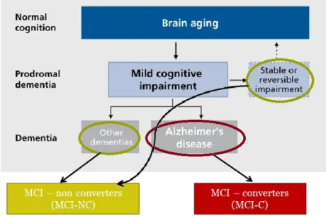
1.1 A conceptual model of possible developments after reaching MCI state. . 3

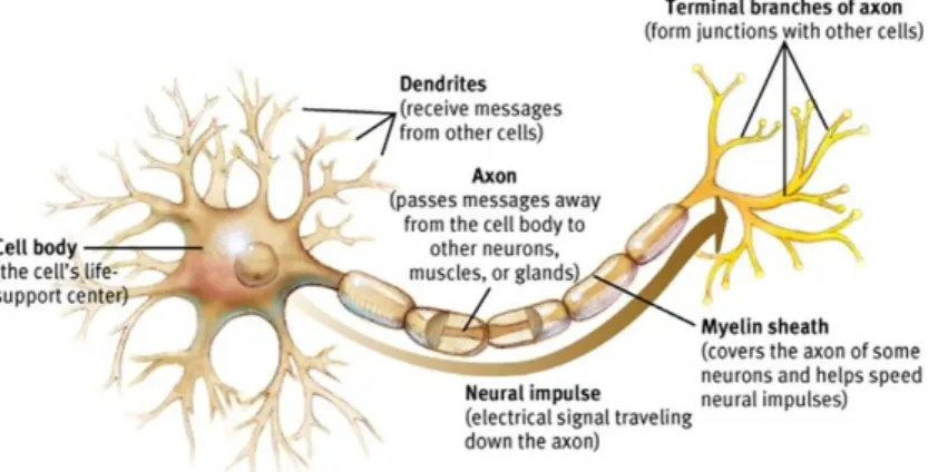
1.2 Structure of a neuron and how the nerve impulse travels. . . 4

1.3 Illustration of the two pathological hallmarks in AD. . . 4

1.4 Illustration of the amyloid cascade hypothesis. . . 5

1.5 Changes in the brain along AD progression and the respective loss of patient capabilities.. . . 6

1.6 Machine Learning framework for neuroimaging classification problems. . . 10

1.7 FDG-PET images demonstrating differences between CN, MCI and AD. . 11

1.8 sMRI images demonstrating differences between CN, MCI and AD. . . 11

3.1 Feature selection for a multimodal (PET + MRI) case. A - Using the L1 norm as the regularization. B - Using L1/L2 norm as regularization. . . . 27

3.2 A 2D representation of the hyperplane xi.w+b = 0 defined by the support vectors and maximum-margin kwk−1 to separate class positive from class negative. . . 29

3.3 Nested Cross-Validation . . . 32

3.4 Representation of the logistic sigmoid function . . . 33

4.1 Representation of the framework for the multimodal classification problems. 41 4.2 Harvard-Oxford cortical (a) and subcortical (b) structural atlases gener-ated by averaging images to MNI152 space. . . 44

4.3 AD vs CN classification results using LR as classifier. . . 48

4.4 AD vs MCI classification results using LR as classifier. . . 49

4.5 CN vs MCI classification results using LR as classifier. . . 49

4.6 MCI-C vs MCI-NC classification results using LR as classifier.. . . 50

4.7 AD vs CN classification results using GP as classifier. . . 52

4.8 AD vs MCI classification results using GP as classifier. . . 52

4.9 CN vs MCI classification results using GP as classifier. . . 53

4.10 MCI-C vs MCI-NC classification results using GP as classifier. . . 53

4.11 AD vs CN classification results using SVM as classifier. . . 55

4.12 AD vs MCI classification results using SVM as classifier. . . 55

4.13 CN vs MCI classification results using SVM as classifier. . . 56

4.14 MCI-C vs MCI-NC classification results using SVM as classifier. . . 56

4.15 Posterior Probabilities obtained with LR for ADvsCN. . . 62

4.16 Posterior Probabilities obtained with LR for ADvsMCI. . . 62

4.17 Posterior Probabilities obtained with LR for CNvsMCI. . . 63

4.18 Posterior Probabilities obtained with LR for MCI-CvsMCI-NC. . . 63

4.20 Posterior Probabilities obtained with GP for ADvsMCI. . . 64

4.21 Posterior Probabilities obtained with GP for CNvsMCI. . . 65

4.22 Posterior Probabilities obtained with GP for MCI-CvsMCI-NC. . . 65

4.23 Subcortical brain regions selected for ADvsCN. . . 68

4.24 Subcortical brain regions selected for ADvsMCI. . . 68

4.25 Subcortical brain regions selected for CNvsMCI. . . 69

2.1 State-of-the-art Multimodal Studies . . . 19

2.2 State-of-the-art MCI Multimodal Studies . . . 22

4.1 Demographic table . . . 38

AD Alzheimer’s Disease

ADNI Alzheimer’s Disease Neuroimaging Initiative

aMCI amnestic Mild Cognitive Impairment

APP Amyloid Precursor Protein

APOE Apolipoprotein E

Aβ Protein beta-Amyloid

CAD Computer Aided Diagnosis

CAP Composite Absolute Penalties

CN Cognitive Normal

CSF CerebroSpinal Fluid

DPC Data sharing and Publications Committe

FAQ Functional Activities Questionnaire

FDG-PET 18F-Fluoro-Deoxy-Glucose Positron Emission Tomography

FN False Negatives

FP False Positives

GM Gray Matter

GP Gaussian Process

GPML Gaussian Processes for Machine Learning

ICP Ishihara Color Plate

IDA Image Data Archive

LASSO Least Absolute Shrinkage and Selection Operator

LIBSVM Library for Support Vector Machines

LONI Laboratory of Neuro Imaging

LR Logistic Regression

MMSE Mini-Mental Status Exam

MNI Montreal Neurological Institute

MRI Magnetic Resonance Imaging

NIA National Institute on Aging

NINCDS-ADRDA National Institute of Neurological and Communicative Disorders and Stroke-Alzheimer’s Disease and Related Disorders Association

PAD Pre-dementia Alzheimer Disease

PIB Pittsburgh Compound B

ROI Region Of Interest

SLEP Sparse Learning with Efficient Projections

SPM Statistical Parametric Mapping

SVM Support Vector Machine

TN True Negatives

TP True Positives

WM White Matter

Greek Symbols

α Lagrange multiplier

λ Regularization parameter

λmax Maximum regularization parameter defined by SLEP toolbox

θ Hyperparameter

θMRI Hyperparameter which defines the weight for MRI data

θPET Hyperparameter which defines the weight for PET data

ξn Slack variable

Roman Symbols

K Kernel matrix

W Feature weight matrix

w Feature weight vector

X Feature data matrix

x Feature data vector

XMRI Feature matrix for MRI data

XPET Feature matrix for PET data

b Bias term

D Data set

d Number of features

L Lagrangian

n Number of samples/subjects

s Weight for a given sample

t Number of tasks/modalities

Introduction

Alzheimer’s Disease (AD) is one of the most common neurodegenerative disorders in older people, accounting for 60-80% of age-related dementia cases (Ye et al.,2011). The disease causes neurons progressive damage or destruction and loss of their connections in the brain, consequently the patient begins losing memory, thinking and behavior abilities and reaches a state that they are entirely unable to take care of themselves, having difficulties controlling even the most basic necessities and consequently, require around-the-clock care. Most often, AD is diagnosed in people over 65 years of age (late-onset), however some individuals younger than age 65 (early-onset) can also develop the disease, but the risk of getting this disease is much higher as people get older. Unfortunately, as neurons normally are not able to regenerate and do not undergo cell division, all the caused damage in the brain cannot be recovered. Therefore, till date AD is considered an irreversible brain disease which leads ultimately to death, because there is currently no known cure and present treatments cannot stop AD from progressing, they only can slow down the worsening of symptoms. The speed of progression can vary, but an average point for survival time ranges from 3.3 to 11.7 years, with most cases in the 7 to 10-year period (Todd et al.,2013).

Brookmeyer in 2007 reported that there were 26.6 million cases of AD in the world in 2006 and in 2050 one person in 85 will suffer from AD (1.2% of total population) or 106.8 million (Cornutiu, 2015). In Portugal the numbers from 2012 indicate that more than 182 000 people suffer with dementia (this represents 1.71% of the population, a little higher than the European mean which is 1.55%) (Alzheimer Europe, 2013). A

report estimates from (World Health Organization (WHO) and Alzheimer’s Disease International,2012) point that the numbers from 2012 will double until 2030, and more than triple by 2050. As most of the AD diagnoses are late, it increases the difficulty of applying some strategies which are used actually to try reducing the progression of the disease. For this reason and due to its big emotional and financial impact on society, AD is a quite concerning public health issue and has been identified as a research priority (Ballard et al.,2011).

Patients suffering from AD at a prodromal stage, i.e. when early symptoms appear and might indicate the start of the disease before the characteristic symptoms occur, are, mostly, clinically classified as amnestic mild cognitive impairment (aMCI). When refer-ring to a patient with MCI it means that the patient has an early loss of brain function before meeting criteria for the diagnosis of dementia. In most cases, the function lost is memory, thus, commonly it can be named as aMCI. These patients show cognitive de-cline greater than expected for their age and education level, however these alterations are not severe enough to interfere with everyday activities (Alzheimer’s Association, 2016). According to (Petersen et al., 2010) study, they suggested that about 16% of elderly people with no dementia are affected by MCI and that approximately two-thirds of those with MCI have aMCI. Studies have also compared the rate of conversion of MCI, they have shown that MCI patients convert to AD at an annual rate of 10-15% per year compared with healthy controls who develop dementia at a rate of 1–2% per year (Bischkopf et al.,2002). So, older MCI patients are at a greater risk of developing AD. The patients that do indeed convert to AD are named as MCI-converters (MCI-C). However, not all MCI patients will develop AD, some either develop other forms of dementia (Vascular dementia; Dementia with Lewy bodies; Parkinson’s disease; Hunt-ington’s disease), remain stable, or in a small minority, revert the process and go back to normal cognition, so these are seen as MCI-non converters (MCI-NC), figure 1.1 de-scribes this division. It is unclear why some MCI patients develop AD or other dementia and others do not (Alzheimer’s Association,2016).

1.1

Alzheimer’s Disease

AD is named after the German physician Dr. Alois Alzheimer, who first described this disease in 1906 (Hippius and Neund¨orfer,2003). He detected a dramatic shrinkage of the

Figure 1.1: A conceptual model of possible developments after reaching MCI state. They can convert to AD (MCI-C) or not (MCI-NC). Adapted from (Golomb et al.,2004)

brain and abnormal deposits in and around nerve cells when analysing the autopsy of a patient who had profound memory loss and many psychological changes. Since then, scientist have been investigating how AD affects the brain, trying to understand its real cause and also several efforts to know how it can be treated are being made, but still with little or no success.

In a healthy adult brain there are around 100 billion nerve cells (neurons), which are the core structural and functional components of the brain and the nervous system. Typ-ically the structure of a neuron consists of dendrites which receive the neural signal, a cell body that will process the signal and an axon which will pass the signal electrically through the neuron and when the electrical signal reaches the end of the axon this causes the terminal branches to release chemical messengers called neurotransmitters. There-fore, the neural communication actually involves an electrochemical communication. An example of a neuron is presented in figure 1.2. In turn, these cells can connect to each other by spaces called synapses, which count for approximately 100 trillion (Alzheimer’s Association, 2016). The neurotransmitters travel across these synaptic clefts and bind to the receptors present in the dendrites from neighbour neuron’s. This transmission will cause the other neuron to become electrically active and the same process continues and passes through other neurons.

Figure 1.2: Structure of a neuron and how the nerve impulse travels. (http://www.appsychology.com/Book/Biological/neuroscience.htm)

The exact cause of AD is still to be fully understood. However, based on several research done for AD along these years, two pathological hallmarks are known: the accumulation of plaques of the protein beta-amyloid (Aβ) outside neurons and the formation of an abnormal form of the protein tau (neurofibrillary tangles) inside the neurons (Ballard et al.,2011). See figure 1.3for illustration.

Figure 1.3: Illustration of the two pathological hallmarks in AD: formation of amyloid plaques betwen neurons and neurofibrillary tangles inside the neurons. (http://www.brightfocus.org/alzheimers/)

The first hypothesis about the amyloid plaques suggested that the total amyloid load had a toxic effect on neurons and consequently lead to neurons failure. With more studies in this area, the pathological changes were more deeply investigated, more precisely the

(Aβ) processing, and a more detailed hypothesis was formulated: the amyloid cascade hypothesis. According to this hypothesis, the protein (Aβ) results from the cleavage of the amyloid precursor protein (APP) and accumulates inside neuronal cells but also extracellulaly where it aggregates into plaques and is believed to interfere with the neurons communication by causing synaptic dysfunction and neuronal death (figure 1.4).

Figure 1.4: Illustration of the amyloid cascade hypothesis. Illustration from (Ballard et al.,2011).

The tau tangles are believed to unable the transport of nutrients and other essential molecules inside neurons contributing therefore for their death.

These processes and changes in the brain are progressive. The first changes can oc-cur without the patient feeling it (clinically silent), as the brain tries to compensate the caused damages (Alzheimer’s Association, 2016). However, as the process starts evolving, the brain can no longer compensate the damages and the first symptoms start appearing in accordance to the brain regions affected. A scheme of the affected areas along AD progress and the symptoms are presented in figure 1.5.

The first areas affected are normally in the medial temporal lobe from the brain cortex, which suffers a shrinkage. More specifically the hippocampus is quite affected. As this part of the brain plays a key role in formation of new memories, patients start having difficulties in storing short-term memories. As years pass more neurons are affected from other brain areas like lateral temporal and parietal temporal lobes; consequently the patient begins suffering some difficulties in other activities like reading and recognising objects. The disease spreads also to the frontal lobe. The frontal lobe is responsible for executive functions such as planning, judgment, decision-making skills, and attention.

Figure 1.5: Changes in the brain along AD progression and the respective loss of patient capabilities. (http://my-dementia.co.uk/Stages%20and%20Cases.html)

Consequently, in this phase, all these functions can decrease drastically. In a more severe stage the disease reaches the occipital lobe and difficulties in seeing clearly rise.

The diagnosis of AD, at present, can only be done with certainty in autopsy by perform-ing a histopathological confirmation, which involves a microscopic examination of brain tissue. Thus, clinically, only probable diagnosis is possible. In addition, as this disease is quite complex and not fully understood, a single medical test will not be sufficient. The diagnosis has to be carefully evaluated by a physician, normally along with a neurologist help, by following some established guidelines. In this context, the physician can require many different tests and patients’ family help, in particular, as explained in (Alzheimer’s Association, 2016), these include: 1- Obtaining medical background (including psychi-atric and cognitive history) and family history from the patient; 2- Requesting a family member or an person close to the patient to describe the changes in thinking skills and behavior; 3- Executing cognitive tests and physical and neurologic examinations; and 4-Acquiring patients’ blood tests and brain images.

1.2

Motivation and problem identification

There is a strong belief that pathological manifestations of AD may appear around 20 or more years before subjects become symptomatic (Alzheimer’s Association,2016). Therefore, it is important to find a way to diagnose even before the classical symptoms

appear. An early and accurate diagnosis will allow patients to benefit from new treat-ments or strategies that may delay the progress of the disease. In this sense, the aim of today’s investigations in this area, is mainly to find the best possible methods which will distinguish between MCI-C and MCI-NC, in order to know which patients will develop AD and need treatment in a near future (i.e. within a few years), and target the disease before irreversible damage or mental decline has occurred.

However, unfortunately the task of predicting conversion from MCI to AD is still known to be difficult and presents challenges beyond that of classifying AD and cognitive normal (CN) subjects or even that of classifying AD/CN vs MCI subjects. For that reason many studies have achieved good results distinguishing AD from CN or CN from MCI, but studies which analyzed MCI-C vs MCI-NC still have low classification performances. This difficulty may be due to the “lag” between brain atrophy and cognitive decline (Hinrichs et al.,2011).

From a public health perspective, treatments as well as clinical trials of therapeutics are classified in terms of primary, secondary, and tertiary prevention interventions (Cavedo et al., 2014). Primary prevention aims at reducing the incidence of illness across the broad population by treating the subjects before disease appears, in other words, it tries to eliminate the potential causes of the disease. Secondary prevention aims at preventing disease at preclinical phases of illness. While tertiary prevention is focused on treating the disease when it has been clinically diagnosed. In AD context, is seems obvious that the primary and the secondary preventions are the ones which concern the population because there is still no known cure for AD, and so tertiary prevention interventions are still not very useful. In case of AD, when referring to a primary prevention it means distinguishing between healthy and MCI patients, when referring to a secondary prevention would be referring to detecting MCI subjects which will convert to AD.

1.3

Use of machine learning for early diagnosis

Machine learning is a subfield of computer science which uses algorithms of artificial intelligence to perform pattern recognition, i.e., to identify patterns and regularities in the data in order to build a model that will make accurate predictions on new data.

Recent advances in neuroimaging techniques and image analysis have significantly con-tributed to better understand the factors which change the brain and are associated with Alzheimer’s disease. Combining them with machine learning algorithms will bring enormous help in finding the best process to reach an early diagnosis of this disease. This combination of elements of artificial intelligence and digital image processing gave rise to a relatively young interdisciplinary technology called computer-aided diagnosis (CAD). For this reason, CAD has gained increasing attention in the medical field in order to simplify the task of interpreting test results by constructing a set of algorithms and computational techniques which use pattern recognition to make future predictions and correctly classify a certain patient.

To define a good classification model when using imaging data, five key steps need to be followed: pre-processing of the data, feature extraction, feature selection, classification and finally the evaluation of the performance of the classification results.

The first steps: pre-processing and feature extraction and feature selection are cru-cial to perform when using neuroimaging data because without these most probably good results for classification would be difficult to get. This is because medical images can have noise and intensity-inhomogeneity, and in addition, when comparing different scans they might not all be aligned so pre-processing will overcome these issues. The pre-processing can include: motion correction with realignment, spatial normalization and spatial smoothing. Furthermore, when dealing with CAD, there exists the high dimensional problem of neuroimaging data, as neuroimages are characterized by having high dimensionality, i.e. having a very large number of voxels in each image. Thus, when analyzing pattern recognition for neuroimaging studies, the number of voxels is much higher than the number of scans/subjects available. This leads to two big prob-lems: it will require a large amount of memory and computation time and can lead to overfitting, which means that it gives rise to a model that overfits the training sample and generalizes poorly to new samples. One of the first steps to overcome this issue is by performing feature extraction. This can be done by extracting, for example, some predefined regions of interest (ROI) which can be meaningful for the study. A feature se-lection on the extracted features can then be performed. Feature sese-lection is the process of selecting a subset of features that can be meaningful and relevant for the classifica-tion procedure. The feature selecclassifica-tion is quite crucial for various reasons: it simplifies the model facilitating interpretation; it makes it computationally more effective as it requires

shorter training times and it enhances generalization by reducing overfitting. Hence, an effective feature selection could not only speed up computation, but also improve the classification performance (Liu et al.,2014).

It is also very common to use kernel methods to solve the high dimensionality of image data. Kernel methods consist of a collection of algorithms based on pair-wise similarity measures between all examples (feature vectors), summarized in a kernel matrix that will have n × n dimensions instead of data matrix dimensions n × d (n-number of sub-jects/scans; d- number of voxels). Given two feature vectors, a kernel function returns a real number characterizing their similarity. The simplest operation one can perform to measure the similarity between two vectors is a dot product (linear kernel). So, in pattern recognition the kernel matrix is many times used instead of the data matrix to simplify the calculations when using neuroimages data, because it makes the model computationally more efficient.

There are many types of machine learning algorithms like supervised learning, unsu-pervised learning and semi-suunsu-pervised. Unlike in unsuunsu-pervised learning, in suunsu-pervised learning all the training data (i.e. the examples provided to the classifier) are properly labeled by hand (i.e. all examples have their class). It consists in two important steps: training and testing. During the training phase, the algorithm learns some mapping be-tween patterns and the labels and then creates a function that can accurately predict the labels for unseen new patterns. For AD classification problems, the method mostly used is the supervised learning method. Nonetheless, semi-supervised learning algorithms are also recently being tested. Furthermore, in supervised learning we can have two types of pattern recognition: classification and regression. If one wants to distinguish classes or subjects (e.g. distinguish MCI from AD) the learnt function is a classifier model and the labels are discrete values, for example -1, 1 for negative class and positive class, respectively. If instead, one wants to predict a specific value (e.g. values of cognitive test scores), then the learnt function will be a regression model and the labels in this case are continuous values.

The final step, after using the classification algorithm, is then to validate it by evaluating its performance. This evaluation is done by performing a cross-validation and looking into the statistics of the model. A good classification model, will present high accuracy (test’s ability to correctly detect or exclude a condition correctly), high sensitivity (test’s

ability to identify a condition correctly) and high specificity (test’s ability to exclude a condition correctly) values. These statistical measurements are calculated by the formulas presented in figure 1.6, where TP is the number of true positives, TN the number of true negatives, FP the number of false positives and FN the false negatives. This figure1.6presents the machine learning framework usually followed for classification problems using neuroimaging data.

Figure 1.6: Representation of the framework for neuroimaging classification problems.

For AD classification studies, a wide range of different medical information could be used as data to distinguish between patients with AD from those who do not have the disease, or to determinate which are more likely to develop AD. These data, in a machine learning context, are normally called modalities, and include: neuroimages, neuropsychological tests, genetic tests, and cerebrospinal fluid (CSF) tests. The two most widely used neuroimage modalities are: 18F deoxyglucose Positron Emission Tomography (FDG-PET) that measures the cerebral metabolic rate for glucose, and structural Magnetic Resonance Imaging (sMRI) which provides information about brain morphometry and therefore can capture brain tissue atrophy related to the loss of neurons (Vemuri and Jack, 2010). Furthermore, these could be used separately or together giving rise to a multimodal classification approach. Existing studies have indicated that different modal-ities can provide essential complementary information and therefore improve accuracy in disease diagnosis, some of these studies will be presented in chapter2. An illustration of these two image modalities is presented in figures1.7 and1.8.

Figure 1.7: Example of FGD-PET images from cognitive normal (left), MCI (middle) and AD (right) subjects. The color scale represents the magnitude of 18F-FDG standardized uptake value ratio (SUVR) which is proportional to glucose uptake. By these images one can identify lower SUVRs in MCI and AD when compared to cognitive normal. Illustration from (Schilling et al.,2016).

Figure 1.8: Structural MRI images from an older cognitively normal (left), an amnestic mild cognitive impairment (middle) and an Alzheimer’s disease (right) subjects demonstrating progressive brain tissue atrophy. Illustration from (Vemuri and Jack,2010).

The feature selection for the neuroimage multimodal case can be performed indepen-dently in each modality. However, this may overloook the complementary information conveyed in different modalities. More recently, studies have used multi-task learning to perform the feature selection for a multimodal approach, where each modality is seen as a task. Multi-task learning is based on a procedure which takes a number of tasks simultaneously and exploits the commonalities between them. So the objective is to defect the intrinsic relationship among different tasks, which can lead to a better results than when learning the tasks independently (Liu et al.,2014).

In terms of classifiers, these can also be distinguished by their property of providing a probability. Most of the classification done in AD studies are based in non-probabilistic classifiers (Zhang et al., 2011; Hinrichs et al., 2011; Liu et al., 2014; Jie et al., 2015), which only provide the class that a sample should belong to. Nonetheless, interest in

probabilistic classifiers has been recently presented (Young et al., 2013; Challis et al., 2015) as these may be advantageous in terms of clinical use because they provide addi-tional information, more precisely, a measure of confidence of the prediction made.

1.4

Contribution of Thesis and Thesis Outline

Considering that classification methodologies to distinguish MCI-C from MCI-NC are still in progress (Golomb et al.,2004;Hinrichs et al.,2011;Davatzikos et al.,2011;Young et al.,2013;Zhang et al.,2014;Cheng et al.,2015;Jie et al.,2015), and taking into ac-count the recent interest in probabilistic classifiers (Young et al., 2013; Challis et al., 2015), this thesis proposes the analysis of a multimodal approach to distinguish these two group subjects using non-probabilistic and probabilistic classifiers. More precisely, in this multimodal procedure two modalities will be used as data: MRI and FDG-PET images. For feature selection the group LASSO multi-task feature selection method provided by (Liu et al.,2009.) software will be used to jointly select features between the two modalities from a whole-brain problem. This whole-brain approach is chosen in order to give the possibility of finding new regions of the brain which can be seen as rel-evant features, instead of using just predefined regions. For the classification step, three classifiers will be studied: the Support Vector Machine (SVM) which is the most widely used classifier for neuroimaging studies and represents a non-probabilistic classifier; and two probabilistic classifiers, which are not so widely used as the first one, the logistic regression (LR) and the Gaussian Process (GP). In this thesis essentially four analyses will discussed: the analysis of the feature selection step to achieve the best performance for each classifier, the comparison of the performance of these classifiers, the interpre-tation of the posterior probabilities given by LR and GP, and the investigation of the selected brain regions.

In chapter2the State-of-the-art will be presented. The theory of the methods used and their respective toolbox is explained in chapter3. In chapter4all the performed work in this thesis is depicted. This chapter has three main sections: section4.1which starts by describing the data used in this work, section 4.2 which shows the experimental design followed to implement the methods proposed and section 4.3 that presents the results and discussion. All the results in this last section are for 4 groups: AD vs CN, AD vs MCI, CN vs MCI and MCI-C vs MCI-NC. Each of these for single modalities (PET

and MRI) and for multimodality (PET + MRI). Finally, the conclusion and future work suggestions are presented in chapter5.

The innovation in this thesis is the comparison of the performance of non-probabilistic and probabilistic classifiers in a whole-brain approach using LASSO with L1

regulariza-tion and group LASSO with L1/L2 regularization as the feature selection methods, for

both single and multimodality respectively, and the analyses of the posterior probabili-ties provided by LR and GP.

State-of-the-art

The publication of the National Institute of Neurological and Communicative Disorders and Stroke-Alzheimer’s Disease and Related Disorders Association (NINCDS-ADRDA) criteria in 1984 represented a breakthrough in the diagnosis of AD (McKhann et al., 1984). These criteria established that the clinical diagnosis should be based on certain characteristics: medical history, clinical examination, neuropsychological testing, and laboratory assessments. However, most demented patients were seen by community physicians who often did not detect dementia or misdiagnosed it, and for pre-dementia AD (PAD) detection this criteria did not show enough sensitivity (Alom et al.,2012). In this context, researchers began developing studies which test machine learning methods in order to understand if new guidelines could be suggested to facilitate physicians in the diagnosis process. Presently, with the research done since then, these guidelines from the 1984 criteria were updated with new guidelines established by the National Institute on Aging (NIA) and the Alzheimer Association, in 2011 (Sperling et al., 2011;Albert et al., 2011; McKhann et al., 2011; Jack et al., 2011). According to this criteria, the brain changes due to Alzheimer’s begin several years (20 or more) before symptoms, and suggest that, in some cases, MCI is an early stage of Alzheimer’s, whereas the earlier criteria from 1984 would require the appearance of memory loss and cognitive decline in order to make a diagnosis of AD. Although this new criteria for a preclinical phase of AD is still not used by doctors for clinical diagnosis, it will help a lot for research purposes. These new guidelines also added other tests that could facilitate an early diagnosis, like for example the use of neuroimages.

One of the first studies using machine learning for AD diagnosis was (Shankle et al., 1997). They used machine learning algorithms combined with clinical data such as subjects demographic data (age, gender, education) and neuropathological tests, like Functional Activities Questionnaire (FAQ), the Mini-Mental Status Exam (MMSE), and the Ishihara Color Plate (ICP) tasks, to learn rule sets that would help detect very early stages of dementia from normal aging and the results were as good as or better than any rules derived from knowledge provided by expert clinicians. This demonstrated the importance of exploiting machine learning techniques for AD early diagnosis. Most machine learning studies in this area are making efforts to understand which biomarkers are able to indicate early stages of AD. A biomarker is a biological factor that can be measured to accurately and reliably indicate the presence or absence of disease, or risk of developing a disease (Alzheimer’s Association,2016). Examples being studied for AD include beta-amyloid and tau levels in CSF, genetic risk factors and brain changes detectable by brain imaging techniques. However, the difficulty rises as these indicators may change at different stages of the disease process. In addition, for a biomarker to be validated in order to be used as medical test for clinical diagnosis, multiple studies in large groups of people have to be made and proven that it accurately and reliably indicates the presence or absence of AD. These factors make it difficult to validate biomarkers for AD and researchers are still investigating these promising candi-dates. Although these candidates are not still seen as entirely validated biomarkers for clinical use, they can provide comprehensive information about the disease being help-ful to investigators in machine learning studies and also to physicians and neurologists, specially the neuroimaging techniques, as they also allow the detection of brain changes associated with AD. These techniques will be presented in the following paragraphs. Structural Magnetic Resonance Imaging (sMRI) is an extremely important image modal-ity for AD studies since it helps detecting brain atrophy as it was presented in previous chapter in figure1.8. In AD, brain atrophy occurs in a characteristic topographic distri-bution, it begins in the medial temporal lobe and spreads to the lateral temporal areas, and medial and lateral parietal areas (Cavedo et al., 2014). The most common sMRI measure employed in AD is the atrophy of the hippocampus, recently recommended by the revised criteria for AD as one of the core biomarkers (Albert et al.,2011;McKhann et al., 2011; Jack et al., 2011). In this sense, several studies proposed classification methods to discriminate between patients with AD or MCI and CN based on sMRI like

for example (Kl¨oppel et al.,2008;Davatzikos et al.,2008). Comparing performance re-sults of these studies an other sMRI studies may not be fully correct because they were assessed on different populations. Many factors as: degree of impairment, age, gender, genotype and level of education could be affecting the evaluation of the prediction accu-racy. Therefore, in order to have the possibility to compare different performance results (Cuingnet et al.,2011) studied 10 methods of classification of AD using sMRI with the same population. Most of the methods showed high accuracy in classifying AD and CN, nevertheless at the prodromal stage, i.e. for MCI, their sensitivity was very low. This suggests the need of combination with other modalities, to overcome this difficulty. Functional Magnetic Resonance Imaging (fMRI) has also been used for AD detection. This modality tracks changes associated with blood flow, more precisely, it measures the blood-oxygen-level dependent (BOLD) signal, reflecting the regional neuronal acti-vation and intracortical processing. As a primary prevention biomarker, it still needs considerable research and development work, because it has the issue of possible con-found between normal aging and development of AD-related pathology. Normal aging alters potential fMRI biomarker and alterations that are seen in MCI group are similar to middle aged healthy controls (Cavedo et al., 2014). Therefore, at the moment, the main use of fMRI would be in secondary prevention trials, which is actually the main concern in this area. However, it should be noticed that pathologies other than AD, such as Major Depression, can mimic the symptoms experienced by MCI patients, and have also been shown to induce changes in functional connectivity (Challis et al.,2015). So, further work needs to be done to better understand the relationship between BOLD signal and clinical changes in dementia and non dementia cases.

As already referred in chapter 1 and presented in figure 1.7, another imaging modality widely used for AD detection and study of its progression is 18F-fluorodeoxyglucose (FDG) positron emission tomography (PET). FDG-PET is a functional marker that measures tissue uptake of glucose and can therefore be linked to the detection of cortical synaptic dysfunction. Normally it can reveal hypometabolism in the temporoparietal regions, posterior cingulate cortex, and frontal lobe even prior to atrophy (Schilling et al., 2016). This image modality has been approved in the USA for diagnostic purposes and is sensitive and specific for AD detection in its early stages (Ballard et al., 2011) and revealed to be a good predictor of MCI progression within the next 2 years combining clinical covariates (Shaffer et al.,2013).

In recent years, researches have also studied a new modality called carbon 11-labeled Pittsburgh Compound B (11C-PIB) PET. This modality provides both perfusion and amyloid deposition information. Combining this modality with structural MRI good results were achieved (Liu et al.,2015). However, this study was basically to distinguish between AD vs CN (accuracy 100%) and MCI vs CN (accuracy 85%) and did not explore MCI conversion to AD. The ones that indeed evaluated MCI conversion like the longitudinal study from (Zhang et al., 2014) did not get such good results and showed high sensitivity results (83-100%) but poor specificity (46-88%). This was explained by the fact that positive results of PIB-PET were also present in other patients with other diseases (Lewy body dementia, Parkinson) and also in some normal subjects. For this reason, prior to 11C-PIB-PET being widely used as diagnostic modality it is still important to demonstrate its accuracy, as it is a high cost investigation biomarker. Furthermore, some AD studies were also based on cerebrospinal fluid (CSF) biomarkers. At present there are three main CSF possible biomarkers for AD molecular pathology: total tau protein (T-tau) that reflects the intensity of neuronal degeneration; hyperphos-phorylated tau protein (P-tau) that probably reflects neurofibrillary tangle pathology; and the 42 amino-acid-long form of amyloid beta (Aβ42) that is inversely correlated with

Aβ pathology in the brain (Cavedo et al., 2014). So, when using this modality for AD prediction these are the ones which are used as CSF features, like it was done in (Cheng et al.,2015).

In addition, genetic factors play an important role in late onset Alzheimer’s disease ( Al-bert et al.,2011). Variants of the apolipoprotein E (APOE) gene, found on chromosome 19, are known to affect the risk of developing AD. These are: APOE ε2, which is rel-atively rare and may provide some protection against the disease; APOE ε3, which is the most common allele, and is believed to play a neutral role in the disease (neither decreasing nor increasing risk); and APOE ε4, which is the strongest known genetic risk factor for AD and present in about 25% to 30% of the population and in about 40% of all people with AD (Liu et al.,2013;Crenshaw et al.,2013). So people who develop Alzheimer’s are more likely to have an APOE ε4 allele than people who do not develop the disease.

Neuropsychological assessments have been used to grade the cognitive state of patients (Folstein et al.,1975) and to characterize dementia associated with AD in several studies

(Shankle et al.,1997;Salmon and Bondi,2009;Chapman et al.,2010;Weintraub et al., 2012). A very common neuropsychological test is the MMSE already mentioned in this chapter when referring to (Shankle et al., 1997) study, one of the first using machine learning methods for AD diagnosis. The neuropsychological tests have proven to be extremely useful to identify the cognitive profiles, determine patterns of impairment, assess changes of impairment over time and also after treatment, and in fact, have been widely used clinically to achieve a probable diagnosis of the disease (McKhann et al., 2011). These are normally the preferred assessments used clinically because they present some advantages and facilities like being inexpensive in comparison with other types of exams, as neuroimaging, and are totally innocuous for the patients, compared to invasive tests like nuclear medicine imaging.

Almost all of the data from these different modalities described above, used as predictors for the disease, can be found in Alzheimer’s Disease Neuroimaging Initiative (ADNI) data repository (http://adni.loni.usc.edu/data-samples/access-data/). All ADNI data is archived in a secured and encrypted system through Image Data Archive (IDA), of the University of Southern California’s Laboratory of Neuro Imaging (LONI), and can be accessed with proper authorization provided by ADNI Data sharing and Publications Committee (DPC). This well-curated scientific data repository is remarkably successful across the globe, and has been a huge help for studies in this area providing data since 2004. According to (Murray, 2012) more than 1300 investigators have been granted access to ADNI data, resulting in extensive download activity that exceeds 1 million downloads of imaging, clinical, biomarker and genetic data. ADNI has data of AD, MCI patients and elderly cognitive normal (CN). These participants are followed and reassessed over time to track the pathology of the disease as it progresses.

2.1

Multimodality

Given that different modalities can help in the detection of different characteristics, an approach combining more than one modality would be preferable. Multimodal neu-roimaging, which is the combination of more than one image modality, may play an important role with regard to early and reliable detection of subjects at risk of develop-ing AD, for two important reasons. Firstly, neurodegeneration in AD cannot be reduced to a singular pathological process in the brain (Cavedo et al., 2014). Thus, different

modalities can detect different important neuropathological aspects which can facilitate the detection of the disease. Secondly, it is well accepted that the onset of appear-ance of these different neuropathological aspects in the brain may occur subsequently and not simultaneously (Cavedo et al.,2014). Therefore, depending on which stage the disease is, one modality may detect a certain pathological characteristic better than other. Intuitively, integration of more than one modality may uncover the previously hidden information that cannot be found using just a single modality. In this context, multimodality is seen as a very useful tool to achieve better classification performances (Zhang et al.,2012;Cavedo et al.,2014;Uluda˘g and Roebroeck,2014). Several studies have exploited the fusion of the multiple modalities to improve AD or MCI classification performance. Some recent studies which use multimodality are presented in table 2.1. It is possible to see how using different modalities allows better results. For example, (Jie et al.,2015) tests two different multimodal cases MRI+PET and MRI+PET+CSF, using the same population, and shows that the second presents better results. In com-parison with single modality, the multimodal approach requires a more careful handling of the data as in this case data from different modalities have to be joined and the num-ber of features given to the classifier rises. The simplest way to combine the data, which was done in many studies (Bouwman et al.,2007; Vemuri et al.,2009; Walhovd et al., 2010) is by concatenating all the features of each modality in the same vector. Other more powerful methods include allocating kernels for each modality and then using a multi-kernel learning method to aggregate all kernels in one only kernel like it is done in (Hinrichs et al.,2011;Zhang et al.,2011).

Study Subjects Modalities Classifier AD vs CN MCI vs CN MCI-C vs MCI-NC

Zhang et al., 2011 51 AD + 99 MCI + 52CN MRI + PET SVM 90.6% — — Zhang et al., 2011 51 AD + 99 MCI + 52CN MRI + PET + CSF SVM 93.2% 76.4% — Hinrichs et al.,

2011 48 AD + 66 CN MRI + PET SVM 87.6% — — Hinrichs et al., 2011 48 AD + 66 CN MRI + PET + CSF+ APOE +

Cognitive scores SVM 92.4% — — Huang et al., 2011 49 AD + 67 CN MRI+PET SVM 94.3% — — Zhang et al., 2012 45 AD + 91 MCI + 50CN MRI + PET + CSF SVM 93.2% 83.2% — Gray et al., 2013 37 AD+ 75 MCI+ 35 CN MRI+ PET+ CSF+ genetic RF 89.0% 74.6% 58.0% Liu et al., 2014 51 AD+ 99 MCI+ 52 CN MRI+ PET SVM 94.4% 78.8% 67.8% Jie et al., 2015 51 AD+ 99 MCI+ 52

CN MRI+ PET SVM 95.0% 79.3% 68.9% Jie et al., 2015 51 AD+ 99 MCI+ 52

CN MRI +PET+ CSF SVM 95.4% 83.0% 72.3%

2.2

Feature Selection

As stated in the previous chapter, feature selection is a crucial step prior to any classi-fication performed on high-dimensional data, because it reduces the number of features given to the classifier, leading therefore to sparse representations of data. As stated in (Yu, 2003), since 1970’s the problem of feature selection has been extensively studied by the machine learning community and it has been proven that it can be effective to remove irrelevant and redundant features.

For neuroimaging studies there are essentially two ways of dealing with feature selection depending on the feature extraction chosen: 1- extracting specific brain regions, which are called regions of interest (ROI) and then performing feature selection in these regions; 2- using feature selection methods to select only the important features of the whole-brain. Many researchers opt for the first approach (Zhang et al.,2011;Zhu et al.,2015; Lahmiri and Boukadoum, 2013; Young et al., 2013) to avoid the high dimensionality problem. For example, in (Zhang et al., 2011) they select 93 ROIs and then average intensity of each ROI region having in total just 93 features for each neuroimage modality, in (Young et al.,2013) they choose to select 10 regions according to (Braak and Braak, 1995), therefore reducing drastically the computational time. However this approach can have some issues. First if there are no ROI’s known a priori, and second having ROI’s a priori will not give the possibility to find new important regions. On the one hand, it can be logical and facilitating to use just ROI’s because they are based in previous studies which have proven a certain theory driven assumptions of which areas are most involved in the disease, nonetheless, research must be done not only to confirm findings but also to expand them, specially for AD case, where absolute knowledge is still on construction. Therefore, a whole-brain analysis may give new and interesting information, in addition to the one already known. On the other side, choosing to design a whole-brain classifier is quite challenging as it will present a lot more features. Typically the consequence is an overfitting of the data, leading to high accuracies for data used in designing the classifier, but poor classification accuracies for new independent test data. To overcome this problem, there is a huge need to use of feature selection methods.

A well-known method is the Least Absolute Shrinkage and Selection Operator (LASSO) method, introduced in 1996 (Tibshirani, 1996). This method uses a regularized L1

regression problems in several studies, but also has become popular topic in the context of classification problems. For the regression problems the most popular loss function used is the least squares estimate (Schmidt,2005), for classification problems, however, least squares estimate may not be adequate, as it gives poor predictions compared to other loss functions, like logistic regression (Rosasco et al., 2004). The comparison of the L1 penalty and the L2 penalty was also performed, and results showed that models

produced with L1 penalty often outperformed the ones produced with L2. (Schmidt,

2005).

Further work have also extended the LASSO for multi-task problems by using other regularization parameters, in particular the L1/Lq regularization, with 1≤ q ≤ ∞,

proposed by (Yuan and Lin,2006) for regression and extended for classification in (Meier et al., 2008). The L1/Lq regularization belongs to the composite absolute penalties

(CAP) family. When q=1, this extension is equivalent to the L1-penalty problem; when

q>1, the L1/Lq regularization promotes group sparsity in the resulting model, which

is quite desirable in many applications of classification problems. Studies analyzed also the influence of different values for q. For example, the results of (Liu and Ye, 2010) showed that smaller values of q had lower balanced error rates then higher values of q. Another study also performed this analysis of the q values, in this case for a multi-task learning with large scale experiments (Vogt and Roth,2012), and the results also showed better results for lower values of q more precisely for values between 1.5 and 2. Thus, L1/L2regularization seem to be the preferred choice to use for the model creation. This

L1/L2norm penalty was already used for AD studies. In (Zhou et al.,2011) they used it

for regression, specifically they tested a multi-task regression problem predicting disease progression measured by cognitive tests. This method of using LASSO with the L1/Lq

penalty for multi-task is also known as the the group LASSO multi-task method or just group LASSO, for simplification.

2.3

Classifiers

Most of machine learning studies carried out for AD classification from neuroimaging problems used the Support Vector Machine (SVM) algorithm as the classifier (Zhang et al., 2011; Hinrichs et al., 2011; Liu et al., 2014; Jie et al., 2015), due to its good accuracy, ability to cope with very high-dimensional data (several features and small

number of examples) as it uses kernels, and for providing a unic solution every time the problem is solved with the same inputs and same conditions. In fact, all studies presented in table2.1used SVM as the classifier, expect for (Gray et al.,2013) which used random forest (RF). Although SVM can bring good results and has big advantages, this classifier is a non-probabilistic binary classifier which uses a supervised learning algorithm, and the use of other classifiers, like probabilistic classifiers, could also be helpful for these kind of studies.

One example is Logistic Regression (LR) which is able to predict, given a sample input, a probability distribution over a set of classes, rather than only outputting the most likely class that the sample should belong to. So, it provides classification with a degree of certainty. Nonetheless, it is worth noting that LR should not be used when there are a large number of features in comparison to the number of training samples, because of the problem of overfitting. In this sense, sparse models are necessarily needed for neuroimaging pattern recognition studies, which is achieved by adding regularization parameters as described above in section2.2. In (Rao et al.,2011) they tested LR with L1 and also another penalty, the L2, for classification of AD vs CN based on sMRI,

and presented classifications with better accuracies when using L1than when using only

the L2 regularization. Furthermore, (Ryali et al.,2010) used LR with a combination of

L1 and L2 norm regularization for whole-brain classification of fMRI data, however not

for AD applications. With their work they could identify relevant discriminative brain regions and accurately classify fMRI data.

Study Subjects

(MCI-NC; MCI-C) Modalities Conversion period Accuracy AUC

Nho et al., 2010 355 (205; 150) MRI + APOE+ family history 0-36 months 71.6% — Zhang et al., 2011 99 (56, 43) MRI + PET + CSF 0-18 months (sens 91.5% spec 73.4%) — Davatzikos et al.,

2011 239 (170, 69) MRI + CSF 0-36 months 61.7% — Hinrichs et al.,

2011 119

MRI + PET + CSF+

APOE +Cognitive scores 0-36 months — 0.7911 Ye et al., 2012 319 (177, 142) MRI+ APOE+

cognitive scores 0-48 months — 0.859 Young et al., 2013 143 (96, 47) MRI+ PET +APOE 0-36 months 74.1% 0.795 Cheng et al., 2015 99 (56, 43) MRI + PET + CSF 0-24 months 80.1% 0.852

Table 2.2: Performance of different state-of-the-art Multimodality studies for predicting MCI conversion to AD.

Recently two papers have also explored another classification algorithm for AD studies: the Gaussian Process (GP). Gaussian Process is a probabilistic classifier and can be seen as a Kernelised Bayesian extension of logistic regression. The first study to use GP for AD applications was (Young et al.,2013). They tested GP in a multimodality

study using MRI, PET, CSF and genetic for classification of MCI-C vs MCI-NC. Their multimodality results were significantly better than any single modality and better than when performing the classification with SVM. Thus, they achieved state-of-the art ac-curacy (table 2.2) and showed that the GP classifier can be successfully applied to the prediction of conversion of MCI patients to AD. Another study (Challis et al., 2015) also used GP classifier, but only for fMRI data and tested different covariance functions. These papers showed that with GP the results were very similar to SVM results or even better. Additionally, they also argue that GP has advantages in comparison to SVM: (i) having a probabilistic classification means that each diagnosis includes an attached degree of confidence rather than a simple binary decision. In case of clinically decision this can be quite useful, as frequently this decision is hampered by overconfidence. (ii) GP is better at finding a set of kernel weights for optimum classification. Rather than finding these through a grid search, like is done when using SVM, with GP a tuning is performed via the likelihood function, which seems to be both more robust and allows a wider search range.

From table 2.1 it is possible to note that the older studies were more concerned with classifying AD vs CN and CN vs MCI. However more recent studies are also concerned in classifying MCI-C vs MCI-NC. Some of the studies performed to predict MCI conversion to AD are presented in table 2.2.

Proposed Methods

In the following chapter the proposed methods will be explained, more precisely each section will present a brief introduction about the basic theory behind each method and the toolboxes used to implement them.

3.1

Feature Selection

The overall goal of feature selection is to overcome the high-dimensional problem by selecting the most important features, i.e., the ones that help minimizing redundancy and maximizing relevance in distinguishing particular conditions of interest. In the case of this work, to distinguish two classes from the study (binary or binomial classification). In this perspective, the goal is to get sparse models, i.e., models that will have zero weights for the features that are not relevant in distinguishing the classes.

3.1.1 LASSO with L1 penalty

Several studies that wish to achieve sparse models, are using the L1 norm penalty as

it has a strong sparsity-inducing property and has shown great empirical success for various applications (Schmidt, 2005; Liu and Ye, 2010). The least absolute shrinkage and selection operator (LASSO) is an example of a model trained with the L1-norm