The comb signaland its Fourier transform

*Correspondence address: Campus da FCT da UNL, Quinta da Torre, 2825-114, Monte da Caparica, Portugal. Tel.:# 351-1-2948520; fax:#351-1-2957786.

Also with INESC.

E-mail address:[email protected], [email protected] (M.D. Ortigueira).

The comb signaland its Fourier transform

ManuelDuarte Ortigueira*

Instituto Superior Te&cnico and UNINOVA, Monte da Caparica, Portugal

Received 25 February 1999; received in revised form 6 October 2000; accepted 8 October 2000

Abstract

In this paper, we study the aperiodic comb signalfrom the point of view of the Fourier transform. The comb is very important in the theory of ideal sampling. The knowledge of its properties is crucial for the establishment of suitable interpolation schemes. Here, we present su$cient conditions so that the Fourier transform of an aperiodic comb is an aperiodic comb. We use this result to propose: (1) an alternative approach to the de"nition of an almost periodic signal and its anharmonic Fourier series; (2) a generalisation of the Shannon}Whittakker sampling/reconstruction for the irregular sampling case. Application of this theory to pulse duration modulation and pulse position modulation is also presented. 2001 Elsevier Science B.V. All rights reserved.

Keywords: Comb; Anharmonic Fourier Series; Irregular sampling; Almost periodic

1. Introduction

The comb signalis one of the most important entities in SignalProcessing, because of its connec-tions with Fourier Series (FS) and idealsampling [8]. The usualcomb is a periodic repetition of the Dirac's delta (generalised) function [10,12]. As is well known, its Fourier transform (FT) is also a periodic comb [1]. In this paper we will study the FT of the generalaperiodic comb signaland formu-late conditions to guarantee that its FT is an aperi-odic comb, too. To see the importance of this subject, let us consider the following practical situ-ation. One of the objectives in electrocardiogram

(ECG) processing is the study of the variability of the cardiac frequency. This is usually done from the so-called RR intervals that are the time inter-vals between peaks of consecutive cardiac beats. These values constitute a time series. We can model the excitation of the heart as a pulse frequency modulation signal. With this, the RR interval signal can be considered as being proportionalto the modulating signal. Therefore, we have a signal that is sampled at a non-uniform spacing: the beat peak positions. Letd

L (n"1, 2,2,¸) be a sequence of RR intervals. Taking 0 as the time origin reference, we de"ne a set of sampling instants:

t

L"tL\#dL t"0,n"1, 2,2,¸ (1.1)

and a signal,v(t)

v(t

L)"dL (1.2)

that is proportional to the modulating signal. In the available commercial systems, the signal v(t) is treated as if it was obtained by uniform sampling.

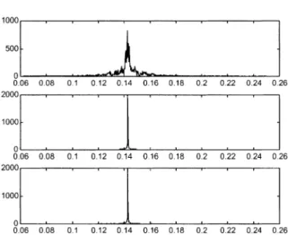
Fig. 1. FFT of a non-uniformly sampled sinusoid (top), FFT of a uniformly sampled sinusoid (middle) and the FT of non-uniformly sampled sinusoid computed through Eq. (1.5) (bottom).

To analyse the error we are making, we took a signal d

L obtained from an ECG signaland con-structed the sequence of instants,t

L, through (1.1). We sampled a sinusoid at those instants and at a uniform spacingn¹, where the sampling interval, ¹, is the mean value ofd

L. For these two signals, we computed their FT by using the FFT. The results are shown in Fig. 1 (top and middle pictures). As it is clear, the use of FFT to compute the FT of the non-uniformly sampled signal is incorrect. To avoid the problem, we assumed that the signalv(t) was ideally sampled by a non-periodic comb

p(t)"> \

(t!t

L) (1.3) obtaining the signal

v

(t)"> \

v(t

L)(t!tL) (1.4) that has the following FT:

< ()"

> \

v(t

L)e\SRL. (1.5) We used this expression to obtain the spectrum shown at the bottom picture in Fig. 1 that shows a good agreement with the picture in the middle. This fact means that the available approaches to studying the variability of cardiac frequency are

intrinsically wrong. These considerations served as motivation for the study we present in this paper. The problem of non-uniform sampling has received increasing attention due to practical applications in real life. The theory of frames [6] has being the most important toolfor dealing with the problem. Here we adopt a more general point of view. We intend to state conditions generalising some of the current results on ideal sampling and reconstruction.

In Section 2, we present the main result of this paper:under stated conditions, the FT of an aperiodic comb is an aperiodic comb [11]. We precise such (su$cient) conditions. The proof is in Appendix A. That result has interesting implications in some well-known"elds, as: almost periodic functions and non-uniform sampling. These subjects are treated in Section 3. In Section 4 we present two applica-tions to communication theory: the pulse duration modulation (PDM) and pulse position modulation (PPM) [2]. Most of the mathematicalbase of the theory is in distribution theory. We present in Appendix B a brief overview of the Axiomatic Theory of Distributions [7,13].

In the following, we represent the sets of integer and realnumbers by Z and R, respectively. The Dirac's symbol will always be represented by(t).

2. The FT of a comb

Consider a set of instants t

L (n"!R,2,

0,2,#R) assumed to form a, as fast as n, increasing sequence such that t

!"$R (for

Theorems 2.1 and 2.2, we only need to assume that the sequence increases faster than(n).

De5nition 2.1. A comb is a distribution, c(t), de"ned by

c(t)"> \

(t!t

L). (2.1)

Theorem 2.1. The series>_\(t!t

L)is convergent. To prove it, let us introduce the function s(t) given by

s(t)">

r(t!t L)!

\ \

r(!t!t

wherer(t) is the ramp function

r(t)"

0 t(0 (2.3)

It is not hard to see that s(t) is a continuous function. In fact, for every"nitet,s(t) is a"nite sum of continuous functions. This means that both the series in (2.2) are uniformly convergent. According, to De"nition B.3 in Appendix B [7,13], the series (2.1) de"ning the comb is convergent, becausec(t) is the second derivative of s(t), that is a continuous function.

The FT (see Appendix B) of an aperiodic comb is an anharmonic [4] FS

C()"> \

e\S_RL (2.4)

Theorem 2.2. The series>

\e\SRL is convergent.

For proof, consider the De"nition B.9 and the series

P()"> \ L$

1 t L

e\SRL (2.5)

As P()(_>

\L$1/tL that is a convergent series, since its terms converge to zero faster than 1/n (t

L(n"!R,2, 0,2,#R) is assumed to

form a, as fast asn, increasing sequence), the series in (2.5) converges uniformly. P() is de"ned by a uniformly convergent series and so it is a continu-ous function. Its second derivative isC() and then the series>

\e\SRL is convergent.

As is well known, the FT of a periodic comb is a periodic comb. We are looking for a generalisa-tion of this result to the non-periodic case. Accord-ing, to what we just wrote above,we are looking for conditions that ensure that the series (2.4) represents a comb. Let us introduce some generality by using the comb

C()"2> \

C

L(!L), (2.6)

where_L is a, as fast asn, increasing sequence, for now. Its FT\is the anharmonic FS

c(t)"> \

C

Le\SLR. (2.7)

We assume that the sequenceC

L is bounded (but not necessarily convergent!) and that, to ensure realness ofc(t),CH

L"C\L and\L"!L.

c(t)"1#2>

C

Lcos (Lt#L) L"arg(CL). (2.8)

Again, the conditions we are looking for must en-sure that (2.7) represents the comb (2.1). If these conditions exist, (2.7) will be a Fourier (nonhar-monic) series associated to (2.1) and (2.4) a Fourier series associated to (2.6).

> \

(t!t L)&

> \

C

Le\SLR. (2.9)

and

2> \

C

L(!L)&> \

e\S_RL. (2.10)

According to the above theorems, all these four series are convergent.

To go further introduce a sequence of intervals I_L andI_L (n"!R,2, 0,2,#R) de"ned by

I_L"]n!

,n#], n3Z (2.11)

and

I

L"]n#,n#], n3Z, (2.12)

where ])] stands for a left-open right-closed

interval.

De5nition 2.2. We de"ne analmost linear sequence (ALS) [4], ¹

$, with uniform density equalto F [5], as a strictly increasing sequence satisfying:

¹

$"tLFtL3ILn3Z,F3R (2.13)

or

¹

$"tLFtL3ILn3Z,F3R (2.14)

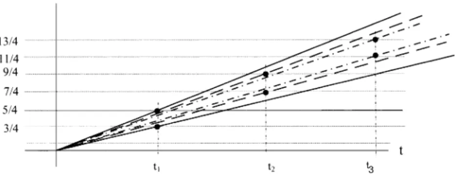
(see Fig. 2).

Fig. 2. De"nition of (2.11) intervals for two di!erent values of the density.

We tried, but failed to prove the conjecture:`everyALS with densityF is a sub-sequence of all the ALS with densitykF, k any integera. In this case the proof of Theorem 2.3 would be simpler.

each intervalof a given set: e.g. t

L3](n!1/4)/ F,(n#1/4)/F]n3Z, for type 1 ALS. For the other set,I

L, we would obtain type 2 ALS.

This is a more precise de"nition than`relatively denseaand has a wider generality than the similar de"nition given by Davis [4]. It is clear that, according to this de"nition, all thet

Lcan be written as

t

L"n.¹#L ¹"1/F n3Z (2.15)

in type 1 case and

t

L"(n#1/2).¹#L ¹"1/F n3Z (2.16)

in type 2 case, with

0)

L(1/(4F)"¹/4. (2.17) If all the

L are zero, the tL sequence will be uniform t

L"n¹"n/F. In the following we will

assume that the sequence of

L has a zero mean value (if the

Lsequence were not zero mean valued, t

L could be written as tL"n¹##L, corre-sponding to a sliding of the whole sequence. So, we do not lose generality with this assumption). In Fig. 2 we show how the intervals are de"ned for di! er-ent values of F(f

'f).

From (2.15) or (2.16), we conclude that the min-imum distance between consecutive elements in an

ALS is equalto 1/2F, while the maximum distance is 3/2F. This means that every strictly increasing sequence with minimum and maximum distances equal, respectively, to

Kand+with+)3Kis an ALS. We compute¹from a given sequence,t

L, by adjusting to it a`stairafunction:

_L"t L!n¹

and forcing_L to have zero mean. Asn¹is an odd function, we force both sequences (corresponding ton'0 andn(0) to be approximated by a stair function. Consider the expressions

lim

,

,

(t

L!n¹)"0P¹"lim

,

2 N(N#1)

,

t L

and

lim

,

,

(!t

L!n¹)"0P¹

"!lim

,

2 N(N#1)

,

t_\ L.

The average of the two is

¹"lim

,

2 N(N#1)

,

(t

L!t\L). (2.18)

De5nition 2.3. We de"ne an almost periodic comb as a comb de"ned on an almost linear sequence.

Theorem 2.3. Ift

Lis an almost linear sequence, there is an almost linear odd sequence

Fig. 3. Sequence of intervals de"ned by (2.23) to compute the almost harmonics from the set of instants.

The even sequence would correspond to a type 2 ALS, that is not suitable here, since"0 (see Fig. 3).

that

FT

(t!t

L)

C

L(!L), (2.19)

where the C

L coe.cients form a bounded sequence and are given by

C I"

1

¹lim

,

1 2N#1

, L\,

e\SIRL. (2.20)

The proof is presented in Appendix A.

Now, it is important to see how to compute the values of_I from the given t

L. We proceed recur-sively for each set of horizontal strips. Consider Fig. 3. The verticalline passing at t

L de"nes with the boundaries of the horizontalstrips two points. These, together with the origin de"ne two straight lines with slopes:

f_IL"k.n#1/4 t

L

(2.21)

and

f IL"

k.n!1/4 t

L

. (2.22)

Forn"1, 2, 3,2compute those slopes and the

pointsK

IL"fIL.tL>andKIL"fIL.tL>. Begin

by computing the intersection of the verticalline passing at t

with the strip centred at k"1. Let

kinteger andk3[K

IL,KIL]. Ifkis odd repeat the procedure for the next n. The sequence of slopes de"ne a sequence of intervals,I

IL: I

IL"]fIQL,fIGL[n"1, 2, 3,2. (2.23)

If this sequence converges, it does so to a degener-ate interval]F

,F[, whereFis the common limit

of the sequences de"ned by (2.21) and (2.22) and it is the frequency of the 1st`almost harmonica. Ifkis even,stop the procedure and go to another ` al-most harmonicafrequency. For the second`almost harmonica, intersect the verticalline passing at t

with the strip centred at. Repeat the procedure.

As it is clear the previous procedure can be used to compute other frequencies (almost harmonic fre-quencies) and we can also conclude that the set of these frequencies is numerable.

3. Consequences

Letx

(t) a signalwith FTX() andtL an ALS. Let us assume that X

() is a bounded function.

We de"ne an almost periodic function, x(t), as the generalised function resulting from convoluting x

(t) withc(t) given by (2.1). Attending to the

prop-erties of thefunction, we can write

x(t)"

L\

x

(t!tL). (3.1)

By the use of Eq. (2.19) we conclude that x(t) is represented by the anharmonic FS [3,9]:

x(t)"> \

x

with

X

L"CL.X(L) (3.3)

However, using (2.1) and the de"nition of FT, we obtain

x

L"c(t)e\SLR

\

x

()e\SLOd

"lim

1 2

>

\

>

\

c(t)x

(s!t)e\SLQdsdt

or, by changing the integration orders and noting that the convolution ofc(t) withx

(t) isx(t):

X

L"lim

1 2

\

x(s)e\SLQds (3.4)

that is the usualway of computing the Fourier coe$cients associated with an almost periodic function [3,9]. Therefore, an almost periodic function is an almost periodic repetition of a basic function.

It is important to remark that the reduction of (3.2) to a trigonometric polynomial is obtained only for signals, x

(t), which are band-limited or have

a FT with nulls at the

L for n'N3Z> (since

X

L_{The dual problem leads to the ideal sampling.}"0). De"ning a signal x

(t) by

x

(t)"x(t).c(t) (3.5)

we obtain after using Eq. (2.19)

X

()"

L\

C

LX(!L) (3.6)

generalising the well-known result. Similarly, insert (2.1) in (3.5) and transforming, we obtain, immedi-ately

X

()"

L\

x(t

L)e\SRL (3.7)

that shows thatX

() is an almost periodic

func-tion. Ifx(t) is a band-limited signal, -BL, we can recoverx(t) fromX

() by ideallow-pass"ltering

provided that *_{2 . So, let} )=) . As,

from (2.20) and (a.9), C

"/2, the "lter must

have a gain equalto 2/and its output is easily obtained from (3.7)

x(t)"

L\

x(t L)

1

5

\5

eHSR\RLd

"

L\

x(t L)

sin[=_(t!t L)] (/2)(t!t

L)

(3.8)

that is the generalisation of the Shannon} Whit-taker cardinalseries. In particular, puttingt"k¹ andt

L"(n#L)¹and noting that¹."2, we obtain

x(k¹)"

L\

x(t L)

sin[.(k!n! L)]

(k!n!

L)

(3.9)

where

"=¹

"

2=

)1. (3.10)

Eq. (3.9) allows us to obtain the values of a signal on a uniform time spacing from an irregular one. If one puts t"t

I"(k#I)¹(k3Z) and tL"n¹ in (3.8), and notes that the sine function is even, we have

x(t I)"

L\

x(n¹)sin[.(k!n!L)]

(k!n!

L)

. (3.11)

A comparison of Eqs. (3.9) and (3.11) leads us to conclude, that under the described circumstances the sine functions appearing in those equations are orthogonal.

4. Applications to pulse modulation

In the following, we are going to study two important cases that fall inside the theory we pre-sented in previous sections. We will present the expressions for the modulated signals in pulse duration modulation (PDM) and in pulse position modulation (PPM) [13].

We will consider the PDM signal with trailing-edge modulation of the pulse duration. The modu-lating signal dependence is on the location, t

I,

to the generalisation of Nyquist criterion stated in (A.11), the sampling instants will be given by (2.15) or (2.16) withFequalto twice the bandwidth of the modulating signal, x(t). In [13], it is assumed t

I!k¹¹, that is a too restrictive relation ac-cording to what we just saw. To correctly represent the PDM signal, we found better to use (2.16), instead (2.15). We consider that each pulse begins at k¹and lasts at

t

I"k¹#¹/2#L, (4.1)

where

L".x(t) (4.2)

with x(t))1 and 0((¹/4. Without losing generality,x(t) is assumed to have a null mean.

It is not a simple task to obtain directly the expression of the modulated signal,s

."+(t). This is

a sequence of rectangular width-variant pulses. However, it is very easy to write its derivative:

s_."+(t)"> \

(t!n¹)!> \

(t!t

L) (4.3)

that can be represented by the Fourier series:

s_."+(t)"1 ¹

> \

e2LR!> \

C

LeSLR (4.4)

easily obtained from (2.9). The Fourier coe$cients are computed from (2.20). Computing the primi-tives of both series in (4.4), we obtain the expression of the PDM signal:

s

."+(t)"S# L$

1

j2ne2LR! L$

C L

j_LeSLR (4.5)

whereS

is equalto 1/2, that is the rectangle mean

width.

The PPM signalis obtained from the PDM signal, by generating"xed width ((¹) rectangu-lar pulses at the end of the PDM pulses. Thus, it is a simple task to observe that

s_."+(t)"> \

(t!t L)!

> \

(t!t

L!). (4.6)

Proceeding as with the PDM signal, we obtain

s

."+(t)"

¹#

L$

C L j

L

eSLR! L$

C L j

L

eSLOeSLR (4.7) or

s

."+(t)"

¹#

L$

C L

j_L[1!eSLO]eSLR (4.8)

that is the Fourier series associated to the PPM signal.

5. Conclusions

In this paper, we studied the aperiodic comb signaland its FT. We showed how we can guaran-tee that the FT of an aperiodic comb is an aperiodic comb. We used this result to propose an alternative approach to the de"nition of an almost periodic signaland computed its anharmonic Fourier series. The original"rst goalof this theory was the gener-alisation of the Shannon}Whittakker sampling/ reconstruction for the irregular sampling case was also presented. Based on the previous results we presented an application to pulse communication by proposing exact expressions for pulse duration modulation and pulse position modulation signals.

Appendix A. Proof of Theorem 2.3

Before going into the proof, we introduce the long-term average (LTA) [9] or mean value [3], g, of a generalised function,g(t), by

g"lim

1 2

\

g(t) dt. (A.1)

A more rigorous statement would write

g"lim

1 2

>?

\ >?

g(t) dt

and the convergence would be uniform in. How-ever, as we work in the "eld of the generalised functions, this subject is not important. With (A.1), it is easy to show that

eSLRe\SIR"

L"I.

For proof of Theorem 2.3, assume that (2.19) is valid. Computing the inverse FT of both members, we obtain

> \

(t!t L)">

\

C

LeSLR. (A.3)

Multiplying both members of (A.3) by e\SLR and computing the LTA, we obtain

\

(t!t

L)e\SIR

L\

C

LeSLRe\SIR

Using (A.2 ) the right-hand side in (A.4) isC I, that, by using (A.1) leads to

C

I"lim

1 2

(t!t

L)e\SIRdt (A.5)

that is the formula to compute the Fourier coe$ -cients [3,9]. If the frequencies_I k"1, 2,2, are multiples of a given frequency , we obtain the ordinary (harmonic) FS. Now, write"(N#

)¹.

Performing the computation, we obtain

C I" 1 ¹lim , 1 2N#1

, L\,

e\SIRL. (A.6)

The sequenceC

Lis bounded which guarantees the convergence of the series in (2.9) and (2.10). In fact C

L)1/¹. We are going to give an interpretation to Eq. (A.6).

(a) The signaleSIRL is the result of sampling a cisoid eSIRin a time spacing that is an ALS. Eq. (A.4) represents the average of those values. (b) When performing the summation in (A.6) we are adding unitary vectors in the complex plane. The resulting vector is, in general, of

"nite length, even if we extend the summation toR. This does not happen if the vectors are collinear, or in a more general situation, if all their extremities lie in the same complex half plane (right or left). If the vectors are collinear, the resulting vector will have a length equal to the sum of the lengths of all the vectors; other-wise, the resulting vector will have a length inferior to the sum of the lengths. Assuming thatt

Lhas the form (2.15) or (2.16) withL hav-ing zero mean, the length of the resulthav-ing vector will be equal to the sum of the real parts of the

vectors and so

C I" 1 ¹lim , 1 2N#1

, L\,

cos(

ItL), (A.7)

where

ItL"2fItLandfItLsatis"es (2.13) or (2.14) for alln,k3Z. As the"rst member in (2.19) is given by (2.4) and using the LTA de"nition we can write

1"lim

5

1 2=

5

\5 2>

\

C

L(!L)eRISd (A.8)

Now, write"(N#

)and perform the

compu-tation to obtain

1"2

lim

,

1 2N#1

, I\,

C

IeSIRL n3Z (A.9)

that is valid for every n3Z. Inserting (A.6) into (A.9), we obtain after some manipulation:

1"2

¹ lim

,+

1

(2N#1)(2M#1)

; ,

K\, + I\+

e\SIRK\RL n3Z. (A.10)

According to the considerations we did before concerning the interpretation of the summations as vectors, we conclude that in the ,

K\,

+

I\+e\SIRK\RLonly the terms corresponding to t

K"tL, contribute to the limit. This is not di$cult to observe. We have

K\, + I\+

e\SIRK\RL

+ I\+

e\SIRK\RL

"(2N#1)(2M#1).

But the terms corresponding tot

K"tL, contribute with the value 1 independently of

I. So, ,

K\,

+ I\+

1"(2N#1)(2M#1)

and the other terms add to zero:

, K_K\_$L,

+ I\+

e\SIRK\RL"0 n3Z.

This is a consequence of the fact that t

K!tL" (m!n)¹#

K!L where K!L3]!, [ (m,

corresponding vectors are likely to have their ex-tremities almost uniformly distributed on the unit circle, so adding to zero. It is easy, now, to obtain the important formula

2

¹"1 (A.11)

which is the generalisation of the Nyquist result obtained in the uniform case. Consider (A.9) again, multiply both sides by e\SKRL, compute the average value and use (A.10)

1

¹lim

,

1 2N#1

, L\,

eSIRL

"1

¹lim

,

1 (2N#1)

, I\,

C I ,

L\,

eSI\SKRL.

The LHS isC

K. So, ifIOKO0 from the second member we conclude that

lim

,

1 2N#1

, L\,

eSI\SKRL"0 kOm, (A.12)

which states orthogonality between two di!erent sinusoids sampled at the same points and is the discrete-time version of (A.2). As _I is an ALS sequence

I"k#I k3Z,I(/4, and"0. (A.13)

_I!

K"(k!m)#I!K with I!K(

/2, ensuring that, witht

L an ALS, the extremities of vectors in (A.8) are likely to be at any point on the unit circle, leading to a null average of the vectors. Eq. (A.13) "xes only the format of the

I sequence; it does not mean that all the corre-sponding `almost harmonicsa exist, because the respective coe$cients may be zero. For example, consider the `extremea sequence t

L"n¹$¹/4, with the signal $ being selected randomly or irregularly. In this case, the "rst almost harmonic has a null coe$cient.

Appendix B. On the axiomatic theory of distributions

B.1. Motivation

In the following, we will present a brief overview on the axiomatic theory of distributions. Although

this theory was developed by Prof. J. Sebastiao and Silva [13] in the 1950s, it remains almost unknown in the engineering community. However, in our opinion, it is the most intuitive and direct of the approaches to distributions. Davis [5] proposed an approach that we consider to be a particular case of the theory we are going to present. The idea under-lying the axiomatic theory of distributions is very simple: `enlarge the class of functions in order to make possible to di!erentiate inde"nitely any continuous functiona.

To begin letIbe an intervalinR,C(I) the set of continuous functions on I and CN(I) the set of functions p times continuously derivable in the usualsense. We represent byDthe operator d/dt. So, a functiong3CN(I) can be represented by

f"D_Ng, (B.1)

where f3C(I). The right inverse operator of D(primitivation operator) is represented bySand satis"es

SNf"g (B.2)

with

Sf"

f() d. (B.3)

As the primitive of a given function is de"ned aside a constant, the setC(I)"Sf#K:f3C(I),K con-stant is contained in C(I) :C(I)MC(I). De"ning the powers of the operator S by the recursion:

SLf"S(SL\)f, with Sf"f and denoting by

P

L\ the set of (n!1)th degree polynomials, we

will have

CL(I)"SLf#p:f3C(I) andp3P

L\, (B.4)

whereC_L(I) is the set of then times continuously di!erentiable functions inR. Putting, now,C(I) as the intersection of all the CL(I)(n"1,2,R), we conclude that

C(I)MC(I)M2MCL\(I)MCL(I)

MC_L>(I)M2MC(I).

consists essentially in prolonging the previous sequence to the left in order to obtain

C

(I)M2MCL>(I)MCL(I)

MC

L\(I)M2MC(I)MC(I).

We represent by C

(I) the reunion of all the

C

L(I)(n"1,2,R) say, the set of all the ` func-tionsathat result from the repeated application of the operatorDtof3C(I).

De5nition B.1. The elements3C

(I) such that "DNf p3N

, f3C(I), (B.5)

we will call generalised functions or distributions (GF).

Therefore, any distribution is a derivative of a continuous function. Example: the second-order derivative of the function x(t)"t is twice the Dirac impulse.

B.2. The axioms

With this de"nition, any continuous function is a distribution. These considerations lead us to the intuitive notion of distribution. However, we need a correct formalframework for the GF theory. For this, we introduce two primitive terms:distribution (or GF) and derivative (generalised). The precise meaning of these terms is established when con-structing the referred formalframework. This is based in four axioms, which will be presented, inter-preted and their consequences discussed.

Axiom B.1. Iff3C(I), thenf3C

(I)

Thus,C

(I) is a nonempty set, since it contains,

at least, the continuous functions.

Axiom B.2. For eachf3C

(I), there is an element

Df3C

(I) such that iffhas derivative,f3C(I) in

the usualsense, thenDfcoincides with f.

This is a guarantee of in"nite di!erentiability of any GF. This means that, iffis a continuous func-tion,Dfwill represent a distribution. There exists,

then, an application from C;N

intoC(I) that

associates a distribution"DLfto each pair (f,n) [12]. To the least natural number in these condi-tions, we call degree of the distribution. So, zero degree GF are the continuous functions; the Heavi-side's unit step has degree 1 and Dirac's impulse has degree 2.

Axiom B.3. For each 3C

(I) there is a n3N

and a functionf3C(I) such that

"DLf. (B.6)

We conclude that any distribution is de"ned by sets of pairs (f,n). For example, the Dirac's delta function can be de"ned by the pairs (r, 2) and (u, 1), whereranduare the ramp and unit step functions.

Axiom B.4. If n3N

and f and g3C(I), then we

have DLf"DLg if and only if f}g has the form

f}g"P

L\(t), wherePL\represents a polynomial

intwith degree less thann.

This axiom speci"es what one understands by equality of generalised functions (FG), or, the conditions such that two pairs (f,n) and (g,m) represent the same GF; for example iff(t)"tu(t) the pairs (f, 2), (f, 1) and (f, 0) represent the same distribution.

Consider the simple case of two continuous func-tions de"ned inR. In this case,Df"fandDg"g,

Df"Dg being equivalent to (f}g)"0, or,

f}g"constant inR. Axiom 4 corresponds to accept

and generalise this fact. As DLf"DL>K(SKf) and DKg"DL>K(SLg), we conclude that DLf"DKg, if and only ifSKf!SLg"P

L>K\.

To "nish these considerations relative to the axiomatic it is convenient to say that we would show that it must be compatible and categorical. We do not do it because it is beyond the objectives of this work.

A generalised functionis said to be tempered or of poly-nomialtype if and only if3Rsuch that (t)/t?is bounded whentPR.

fact, it is not possible to de"ne product of two GF in order to guarantee that it enjoys the usual properties (namely, to be associative, to satisfy the product derivative rule and to coincide with usual product when both factors are continuous func-tions. We do not go further (see [7]).

B.3. Sequences and series of distributions

We are going to generalise the notions of limit of a sequence in order to introduce the notion of series.

De5nition B.2. Letf

Lbe a sequence of GF. We will say that f

L converges to f in C(I) if and only if

there existp3N,FandF

L3C(I) such that we have DNF

L"fL,DNF"fand thatFLconverges uniform-l y toFinI.

With this de"nition, we are able to de"ne sum of a series of distributions.

De5nition B.3. Letf

Lbe a sequence of distributions inI. We say that the series

fL is convergent in

C

if and only if the sequence of partial sums

g

I_{If the series is bilateral:}IfL is convergent. _>

\fL, it is convergent, if the series

fL and \\fL are both convergent. The sum of the series is obtained by adding the sums of the two series.

B.4. Fourier transform of distributions

Letbe a GF inR. We de"ne the primitive of

to any GFsuch that

D". (B.7)

The integral _@?(t) dt is de"ned by the gener-alised Barrow formula:

?

(t) dt"(b)!(a). (B.8)

An integralexists or is convergent if and only if both limits exist. It can be proved that if a GF is integrable in R, then (t)"O(t\) when tPR. On the other hand, if there exist(!1 such that

(t)"O(t?) when tPR then is integrable in

R[7].

Similar to the usual procedure, we de"ne FT of a generalised function (t) as being the function

() such that

()"

0

(t)e\SRdt (B.9)

if the integralexists.

De5nition B.4. The integral(t,) dis said to be convergent inRif and only if there exists a primi-tive of relatively to convergent in R when PR.

We will write then (t,) d"(t,#R) !(t,!R) in R. In particular, it can be proved

that

(a) if is summable in R, FT[] exists and it is a continuous bounded function inR.

(b) Ifis a temperedGF, then its FT exists and it is also a tempered GF.

References

[1] R. Bracewell, The Fourier Transform and Its Applications, McGraw-Hill Book Company, New York, 1965. [2] A.B. Carlson, Communication Systems, McGraw-Hill

InternationalEditions, New York, 1983.

[3] C. Cordoneanu, Almost Periodic Functions, Wiley Interscience Publishers, New York, 1968.

[4] A. M. Davis, Almost periodic extension of band-limited functions and its application to nonuniform sampling, IEEE Trans. Circuits Systems CAS-33 (10) (October 1986) 933}938.

[5] A.M. Davis,K

Generalised functions, Proceedings of the

IEEE InternationalConference on Circuits and Systems, Seattle, Washington, DC, USA, 1995, pp. 1652}1659. [6] R.J. Du$n, A.C. Schae!er, A class of nonharmonic

Fourier series, Trans. Amer. Math. Soc. 72 (1952) 341}366. [7] J.C. Ferreira, Introduc7ao a` Teoria das Distribuic7oes,

Fun-dac7ao Calouste Gulbenkian, 1990. English version:

[8] A.J. Jerri, The Shannon sampling theorem*its various extensions and applications: a tutorial review, Proc. IEEE 65 (11) (November 1977) 1565}1596.

[9] B.M. Levitan, V.V. Zhikov, Almost periodic functions and di!erentialequations, Cambridge University Press, Cambridge, 1982.

[10] M.J. Lighthill, Introduction to Fourier analysis and gener-alised functions, Cambridge University Press, Cambridge, 1964.

[11] M.D. Ortigueira, What about the FT of the comb signal?, Proceedings of SAMPTA-97, Aveiro, Portugal, 1997, pp. 28}33.

[12] L. Schwartz, TheHorie des Distributions, Herman & Cie, Paris, 1966.