(will be inserted by the editor)
Calibration of parameters in Dynamic Energy
Budget models using Direct-Search methods
J. V. Morais · A. L. Cust´odio · G. M. Marques
Received: date / Accepted: date
Abstract Dynamic Energy Budget (DEB) theory aims to capture the quan-titative aspects of metabolism at the individual level, for all species. The parametrization of a DEB model is based on information obtained through the observation of natural populations and experimental research. Currently the DEB toolbox estimates these parameters using the Nelder-Mead Sim-plex method, a derivative-free direct-search method. However, this procedure presents some limitations regarding convergence and how to address con-straints.
Framed in the calibration of parameters in DEB theory, this work presents a numerical comparison between the Nelder-Mead Simplex method and the SID-PSM algorithm, a Directional Direct-Search method for which conver-gence can be established both for unconstrained and constrained problems. A hybrid version of the two methods, named as Simplex Directional Direct-Search, provides a robust and efficient algorithm, able to solve the constrained optimization problems resulting from the parametrization of the biological models.
Support for J. V. Morais was provided by FCT/MCTES (PIDDAC) through project UID/EEA/50009/2013.
Support for A. L. Cust´odio was provided by Funda¸c˜ao para a Ciˆencia e a Tecnologia (Por-tuguese Foundation for Science and Technology) under the project UID/MAT/00297/2013 (CMA).
J. V. Morais · G. M. Marques
MARETEC - Marine, Environment & Technology Center, Instituto Superior T´ecnico, Uni-versidade de Lisboa, Lisboa, Portugal
E-mail: [email protected],[email protected] A. L. Cust´odio
Department of Mathematics, FCT-UNL-CMA, Campus da Caparica, 2829-516 Caparica, Portugal
Keywords Dynamic Energy Budget theory · Nelder-Mead Simplex algo-rithm · Directional Direct-Search methods · Constrained optimization
1 Introduction
Models are used to describe and simulate a particular system or process by referencing it to existing knowledge. They can be used as a proxy of the reality and, for this reason, they could be an alternative to direct measurement or experimental processes when simulating the behavior of a system in different conditions.
The conception of a model should start with the statement of a set of as-sumptions, to which follows the mathematical formulation, using the previous assumptions. In a third phase, a sequence of tests on consistency, coherence, parameter sensitivity and relevance should be performed, analyzing the qual-ity and adequacy of the model, like is suggested by Kooijman (2011) . The results of the model should be related to the quantitative aspects that can be measured and it is important to define the adequate experiments to test against the model predictions.
Models are frequently used in Biology to describe and quantify the metabolic processes of organisms and also to predict changes in these processes with the inclusion of variations in the environment. One additional research interest is to relate the physiological processes in an organism with the dynamics at a population level.
The calibration of a biological model consists in the definition of a set of parameters, in an attempt of matching the predicted values computed with the model with observed data. The parameter values obtained with the calibration procedure characterize the corresponding organism.
Considering the diversity of life on Earth, the formulation of a single the-oretical description that could be applied to all organism species seems to be a hard task. However, some similarities, such as von Bertalanffy’s growth curve
(in von Bertalanffy (1957)) and Kleiber’s law on metabolic rate (in Kleiber (1932)), suggest that mechanisms responsible for the control of metabolism are not
species specific (see Sousa et al. (2008)). These evidences and other empiri-cal patterns in Biology suggest that a general approach should be taken when describing energy and mass fluxes inside the organisms. Fortunately, such a general theory has already been developed, namely the Dynamic Energy Bud-get (DEB) theory, authored by Kooijman (2000; 2010)
DEB theory aims to describe the rates at which an organism assimilates and mobilizes energy for somatic maintenance, growth, maturation and reproduc-tion, considering the state of the organism and of the environment. The state of an organism can be characterized by the corresponding size and amount of reserves, while the environment is characterized by distinct factors, such as food availability and temperature (see van der Meer (2006)). The phy-logenetic information of the species allows the formulation of a specific DEB model which permits to relate observed patterns of growth, development,
re-production and mortality in a particular organism to empirical information on feeding rates and maintenance costs, as suggested by Nisbet et al. (2000)
DEB models are based on simple thermodynamic principles and, for this reason, they can be applied to all species, including micro-organisms, plants and animals. In fact, they can be an important tool to describe several ener-getic aspects of the life cycle of an organism. These enerener-getic aspects can be compared through the parameters of the model, which can be estimated using the observational and experimental data available. Additionally, DEB models of organisms can be used in studies of dynamics of structured populations, including optimization of pest control, the development of optimal harvesting strategies, and the reduction of sludge production in sewage treatments, as re-ported in van der Meer (2006) The effects of a concentration of a specific stressor in an organism can also be analyzed with the application of DEB the-ory and measured by changes in parameters values (see Jager et al. (2014) or Baas et al. (2018)).
The estimation of DEB model parameters, based on the adjustment of the predicted values computed with the model to the observed data, is not an easy task. Currently, due to its derivative-free nature, this constrained optimization problem is solved with the application of the Nelder-Mead Simplex method, proposed by Nelder and Mead (1965) and implemented in the DEBtool (available at http://www.bio.vu.nl/thb/deb/deblab/debtool/DEBtool M). However, this algorithm presents some limitations regarding convergence and how to address constraints. For this reason, it is of major importance to develop a systematic, reliable and efficient estimation procedure, which would allow a simple application of DEB theory to several species, in order to maximize the time associated with the biological interpretation and analysis of the results, rather than the time related to the computational work of the estimation procedure.
The Add-my-Pet collection (2018) database was developed to include different species for which the estimation procedure was applied and the corre-sponding parameters obtained. The collection has now more than 1000 species and includes all the needed files for the estimation of parameters.
Using the Add-my-Pet database, the aim of this study is to evaluate the performance of the current procedure used for estimation of parameters in DEB models. The Nelder-Mead Simplex algorithm will be compared with an alternative class of derivative-free methods, namely Directional Direct-Search, for which, under mild assumptions regarding the smoothness of the objec-tive function, convergence can be established both for unconstrained and con-strained optimization. Additionally, some alternative approaches are proposed to develop a convergent and efficient algorithm, able to solve the constrained optimization problems related with the DEB parameters estimation.
This paper is organized as follows. Section 2 defines the calibration of pa-rameters in a DEB model as an optimization problem. Section 3 provides a description of the Nelder-Mead Simplex algorithm and the corresponding lim-itations. Section 4 introduces an alternative class of derivative-free methods, namely Directional Direct-Search. In Section 5, the results of a numerical
com-parison between the two methods are reported, motivating the development of a hybrid algorithm, which is presented in Section 6. Some strategies for addressing constraints are described in Section 7, as well as the corresponding numerical results. Finally, Section 8 is devoted to some concluding remarks and ideas for future work.
2 DEB problem definition
In DEB theory, differential equations are used to describe the quantitative as-pects of metabolism at the individual level, as proposed by Sousa et al. (2010) The model predictions represent the performance of an organism in a variable environment.
In a standard DEB model three life stages are considered: embryo, which neither feeds or reproduces; juvenile, which feeds but does not reproduce, and finally, adult, which both feeds and reproduces. Each organism is described in terms of several state variables, as structural body, quantified as volume (V ), reserves, quantified as energy density (E), level of maturity, expressed in terms of cumulative energy investment (EH), and reproduction buffer, expressed in
terms of energy allocated to reproduction (ER). Maturity has no mass or
energy in the body, however, it controls life stages transitions that cover the full life cycle of the organism.
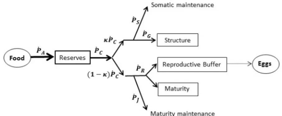
Fig. 1 Schematic representation of the standard DEB model.
Following the standard DEB model introduced by Kooijman (2010) and represented in Figure 1, energy enters the organism as food and it is as-similated at a rate of ˙pA into reserves. The mobilization rate, denoted by
˙
pC, represents the energy mobilized from reserves. According to the κ-rule
of Kooijman (1986) a fixed κ fraction of ˙pC is allocated to pay somatic
maintenance ( ˙pS) and growth ( ˙pG), while the value (1 − κ) ˙pC is used to pay
the costs associated with maturity maintenance ( ˙pJ), maturation ( ˙pR) and,
over the other uses. Growth ceases when the fixed fraction κ just supplies the somatic maintenance demand. The organism may begin to reproduce when a certain maturity threshold is reached.
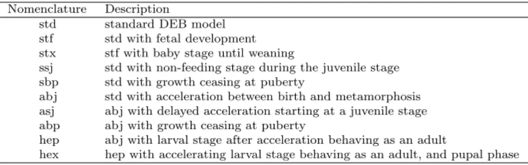
Although the standard DEB model is appropriated to capture many as-pects of the metabolic performance of species, more complex species or differ-ent applications could require extensions to incorporate specific characteristics of organisms. For example, a big number of fish species has an exponential growth phase after birth and this can be modelled by considering a juvenile phase with acceleration. Table 1 specifies the different extensions of the stan-dard DEB model.
Table 1 Different DEB models available in the Add-my-Pet (AmP) database. Nomenclature Description
std standard DEB model stf std with fetal development stx stf with baby stage until weaning
ssj std with non-feeding stage during the juvenile stage sbp std with growth ceasing at puberty
abj std with acceleration between birth and metamorphosis asj abj with delayed acceleration starting at a juvenile stage abp abj with growth ceasing at puberty
hep abj with larval stage after acceleration behaving as an adult
hex hep with accelerating larval stage behaving as an adult, and pupal phase
Following Kooijman (2010) , the different models consider the effects of changes in shape during growth, the inclusion of more types of substrate, reserves or structures, the formation and excretion of metabolic products, the production of free radicals and their effect on survival, and processes of adaptation to the availability of substrates.
For the estimation of DEB parameters, the covariation method has been widely used, linking model predictions with experimental and field observa-tions of distinct life stages of the individual (see, for instance, Lika et al. (2011) or Marques et al. (2018) . The Add-my-Pet option, included in the DEBtool, allows the estimation of parameters by minimizing the difference between ob-served (dij) and predicted values using a DEB model (pij), measured through
a weighted least-squares average, as proposed by Marques et al. (2018) :
minimize (x1, ..., xn)∈ Ω m X i=1 mi X j=1 ωij (pij(x1, . . . , xn) − dij)2 d2 i + p2i(x1, . . . , xn) , (1)
where m represents the total number of data sets, i denotes a specific data set, mi denotes the number of observations in data set i, j represents a given
point on the data set i, and di and piare defined as
di= 1 mi mi X j=1 dij and pi(x1, . . . , xn) = 1 mi mi X j=1 pij(x1, . . . , xn). (2)
These means are used in the denominator so that problems with some dij
equal to 0 can be dealt with. In (1) and (2), x1, . . . , xnrepresent the variables
of the optimization problem, corresponding to the n model parameters to be estimated, and ωij represent weight coefficients associated with the data,
which could be used to introduce a level of confidence on the observed values. In eq. (1) we have symmetrized data and predictions in the denominator. The purpose is to balance the overestimation and the underestimation, without which one can have a bias in estimation and lack of convergence in a realistic part of the parameter space (for more detail see Marques et al. (2018)).
The parameters space is restricted to a subspace Ω ⊂ Rnwhere the mathe-matical DEB model is well-defined and where the parameters have a biological meaning. The constraints defining Ω are dependent on the species under anal-ysis. Nevertheless, there are three general types to be considered:
(1) li + αi ≤ xi ≤ ui − βi, i = 1, . . . , n, with −∞ ≤ li < ui ≤ +∞
αi≥ 0, βi≥ 0
(2) Pn
i=1ajixi+ γj≤ bj, j = 1, . . . , q and γj ≥ 0
(3) gl(x1, . . . , xn) + θl≤ 0, l = 1, . . . , p and θl≥ 0
The constants αi, βi, γj and θl, defined in (1), (2) and (3), are set equal
to a small positive value, when the constraints need to be strictly satisfied. Otherwise, they will be equal to zero.
The constants li and ui in (1) correspond to lower and upper bounds,
re-spectively. Bound constraints (1) are applied to most variables. In fact, most parameters cannot be negative or equal to zero because of its biological mean-ing. Another example is the κ fraction that should always be strictly between zero and one. Although, for some parameters upper bounds are not defined.
Linear inequalities (2) are generally applied to maturity levels, since it is necessary to guarantee that two subsequent maturity levels are not equal. In the standard DEB model, the maturity at birth, Eb
H, should always be
inferior to the maturity at puberty, EHp. Otherwise, the model has no biological meaning.
Finally, (3) represents black-box constraints for which an analytical form is not available for use. In the standard DEB model, one example of this type of constraints is the condition required for birth, which is provided by the model as an oracle type condition: yes, if birth can occur; no, otherwise.
The number of variables, the total number of constraints and the type of constraints depend on the species and on the corresponding model. For example, the abj model includes an additional maturity threshold to describe an intermediate transition between birth and puberty, called metamorphosis, (EHj). Before metamorphosis, the growth curve is exponential and it can not be described by the typical von Bertalanffy growth curve of the standard model. In this case, a new linear constraint must be defined to guarantee that the
maturity level at metamorphosis is strictly between the maturity at birth and the maturity at puberty.
3 The Nelder-Mead Simplex method with restarts
The Nelder and Mead (1965) Simplex algorithm is one of the most popular derivative-free optimization methods. The algorithm proceeds by evaluating points in a simplex, without any explicit or implicit derivative approximation or model building of the objective function. At each iteration, the algorithm attempts to replace the worst vertex of the simplex by a new vertex resulting from a set of geometrical operations performed on the simplex.
The most common variants of the Nelder-Mead Simplex method allow re-flections, expansions and inside or outside contractions of the simplex (see Figure 2). When the previous operations fail in providing a point better than the worst vertex of the simplex, the simplex is shrunk towards its best vertex (see Figure 3).
Fig. 2 Reflection (xr), expansion (xe), outside contraction (xoc), and inside contraction
(xic) of a simplex, used by the Nelder-Mead Simplex method.
Fig. 3 Representation of a shrink operation used by the Nelder-Mead Simplex method.
The Nelder-Mead Simplex algorithm is the standard procedure used for the estimation of parameters in DEB models, being an implementation available in the DEBtool. Algorithm 1 provides a complete description of the variant considered.
Algorithm 1 (Nelder-Mead Simplex algorithm)
Initialization: Choose an initial simplex of vertices X0= {x00, x 1 0, . . . , x n 0}. Choose coefficients: 0 < γS< 1, −1 < δic< 0 < δoc< δr< δe. (3) Standard choices are:
γS = 1 2, δ ic= −1 2, δ oc =1 2, δ r= 1, and δe= 2. (4)
For each iteration k = 0, 1, 2, . . . Evaluate f at the points in Xk = {x0k, x
1 k, . . . , x n k} and define f i= f (xi k), i =
0, . . . , n. Order the n + 1 vertices, such that
f0≤ f1≤ . . . ≤ fn (5)
Compute the centroid xc=
1 n n−1 X i=0 xik.
1. Reflect: Reflect the worst vertex (xn
k) over the centroid (xc), xr = xc+
δr(x
c− xnk). Evaluate fr = f (xr). If f0 ≤ fr < fn−1, replace xnk by the
reflected point and terminate the iteration.
2. Expand: If fr < f0, calculate a expansion point, xe = xc+ δe(xc− xnk)
and evaluate fe = f (xe). If fe ≤ fr, replace xnk by the point xe and
terminate the iteration. Otherwise, replace xnk by the reflected point xr
and terminate the iteration.
3. Contract: If fr≥ fn−1, then a contraction is perform between the best
of xr and xnk. If f
r < fn, perform an outside contraction, x
oc = xc+
δoc(x
c− xnk) and evaluate f
oc= f (x
oc). If foc ≤ fr, replace xnk by xoc and
terminate the iteration. Otherwise, perform a shrink. If fr≥ fn, perform
an inside contraction, xic= xc+ δic(xc− xnk) and evaluate f
ic= f (x ic). If
fic< fn, replace xn
k by xicand terminate the iteration. Otherwise, perform
a shrink.
4. Shrink: Evaluate f at the n points x0
k+γs(xik−x0k), i = 1, ..., n and replace
x1
k, ..., xnk by these points. Terminate the iteration.
The initial simplex is built following the procedure suggested by L. Pfeffer and reported in Fan (2002) . Let Xn×(n+1)store columnwise n + 1 replicas
of the initial vertex x0
0. The initial simplex, X0, is computed as:
X0= X + [ 0 diag (g(x)) ], where (6) gj(x) = ( 0.00025 if (x0 0)j= 0 0.05(x00)j if (x00)j6= 0 j = 1, . . . , n (7)
If the problem has constraints then the initial simplex is modified as xi0 = xi0/2k, with i = 0, . . . , n and k ∈ N0the smallest value which ensures feasibility.
As stopping criteria, the optimization procedure ends when the relative size of the simplex becomes smaller than a chosen tolerance ∆simplex > 0, when
the difference between the objective functions values calculated in the simplex vertices is inferior to a certain tolerance ∆f un > 0, or if a maximum number
of function evaluations is reached. As default values, the DEBtool considers ∆simplex= 10−4 and ∆f un= 10−4.
Despite its good practical performance, the Nelder-Mead Simplex method presents some limitations. Lagarias et al. (1998) established the conver-gence of the original Nelder-Mead Simplex method for strictly convex functions of one variable. However, McKinnon (1998) provided a family of strictly convex examples of dimension two for which the algorithm applied consecutive inside contractions towards a point that is not a minimizer, when considering a specific initialization.
These failures motivated the development of convergent variants of the al-gorithm. In order to avoid the deterioration of the simplex geometry and the convergence to non-stationary points, Price et al. (2002) allowed the algo-rithm to run as long as it provided some form of sufficient decrease, avoiding stagnation. This modified method does not allow shrink operations, replacing them by the computation of quasi-minimal frames. Convergence is a direct consequence of the use of these quasi-minimal frames and it is established for C1functions.
The modified Nelder-Mead Simplex algorithm suggested and analyzed by Tseng (1999) proposes monitoring the simplex geometry for all operations, with the exception of the shrink, where the normalized volume of the simplex is intrinsically preserved. This version is flexible in the number of vertices to retain when computing a new simplex, but again requires sufficient decrease when accepting new points and convergence is established for continuously differentiable functions.
Kelley (1999) proposed a different sufficient decrease condition which, if satisfied for all iterations and if the diameters of the simplices converge to zero, would guarantee convergence of the Nelder-Mead Simplex algorithm to a stationary point, when applied to a smooth function. When the sufficient decrease condition fails and a shrink is due, the method could be in stagna-tion. Kelley (1999) proposes the replacement of this operation by an oriented restart, which numerically improved the robustness of the method.
A restarting strategy is also implemented in the DEBtool when solving problems with the Nelder-Mead Simplex algorithm. The adopted variant restarts the algorithm several times, in consecutive runs, which are not independent. The final point computed by the algorithm in a given run is used as initializa-tion in the next one. Again, the thresholds ∆simplex, ∆f un and a maximum
number of function evaluations are considered as stopping criteria for each one of the considered runs.
Additionally to the convergence problems described, other important dis-advantage of the Nelder-Mead Simplex method is of not being originally de-signed to address constrained optimization problems.
Penalty or barrier functions could be considered as a simple way to extend the algorithm to constrained optimization (see Nocedal and Wright (2006)). Since penalty functions allow the evaluation of infeasible points, its use would be inappropriate in the context of DEB problems. If feasibility is not ensured, the DEB model would not provide meaningful results. The same argument ap-plies to the use of filter methods, proposed by Fletcher and Leyffer˙(2002) Hare (2010) suggested projection techniques to address constraints, which avoid the evaluation outside the feasible region by projecting infeasible points into the boundary. The presence of black-box constraints, for which we do not have an explicit mathematical formulation, prevents the use of this approach. In derivative-free optimization it is common the use of an extreme barrier function defined as
fΩ(x) =
(
f (x) if x ∈ Ω
+∞ otherwise , (8)
only evaluating feasible points, also saving in computational budget. This approach is applied to the Nelder-Mead Simplex method included in the DEBtool, as a way to address constraints. Despite of its easy implementation, the application of an extreme barrier function can cause a rapid degeneration of the simplex form and volume, and increases the probability of not exploring subspaces near to the boundary of the feasible region.
Box (1965) proposed a technique to handle constraints in a variant of the Nelder-Mead Simplex method. This approach, named as the COMPLEX algorithm, is again a simplicial method based on the reflection of the worst point of a generalized structure over the centroid of the remaining vertices, but allowing a larger number of points in the structure (higher than n + 1 and less or equal than 2n). If a trial point is out of the boundaries, it is reset to a value l + 0.000001 if the lower bound is violated, or to h − 0.000001 if the violation respects to the upper bound. Regarding the remaining constraints, if the trial point is infeasible, it is moved halfway towards the centroid of those points already selected, until a feasible point is found. Guin (1968) refined this last idea, applying it not only to general constraints but also to bounds. The procedure should be repeated until the trial point is feasible or a minimum threshold is reached.
Later, Le Floc’h (2012) showed that Box’s method can fail to find a satisfactory solution, considering that it always tries to perform operations too near to the boundary. Guin’s approach can work better in practice but it produces a collapse of the simplex and it tends to fail when the centroid is an infeasible point. Le Floc’h compared these two methods with the use of a penalty function approach, and with a variant of the Box method, called Random Box.
In Random Box, when the trial point is out of the boundaries and the centroid (xc) respects the constraints, the trial point is reset to l + z(xc− l)
when the lower bound is violated, and to h − z(h − xc) when the upper bound
is not satisfied, where z is a random number in the interval [0.000001; 0.5]. If the centroid does not satisfy the constraints, the original Box method is applied. None of the approaches was completely satisfactory, even for simple quadratics.
4 Directional Direct-Search
An alternative class of convergent derivative-free optimization methods is Di-rectional Direct-Search. Instead of using simplices through the iterative pro-cess, sampling is guided by sets of directions with particular geometrical fea-tures, namely positive spanning sets (see Conn et al. (2009)). A positive spanning set is a set of vectors that generates Rn, considering non-negative
linear combinations of its elements. A minimal positive spanning set is named as a positive basis. For continuously differentiable functions, positive spanning sets (and positive basis) are guaranteed to have a descent direction among one of their vectors (see Conn et al. (2009)). This is a key feature, when design-ing convergent algorithms for numerical optimization. A simple example of a Directional Direct-Search method is coordinate search, which uses the positive basis D⊕= [ I − I ], where I represents the identity matrix.
Each iteration of a Directional Direct-Search method is organized in a search step and a poll step. The search step is optional, not required for estab-lishing convergence. Its main purpose is to improve the numerical performance of the method, possibly with the use of some heuristic procedure.
When the search step fails in improving the current best point, the poll step is performed. The algorithm tests the points corresponding to the directions of a positive spanning set, scaled by a step size parameter. If no better point is found, the step size is decreased.
Algorithm 2 provides a description of this class of methods. Algorithm 2 (Directional Direct-Search)
Initialization: Choose x0, α0> 0, and a set of positive spanning sets D.
Define the constants δ1, δ2and δ3, with 0 < δ1≤ δ2< 1, and δ3≥ 1.
For each iteration k = 0, 1, 2, . . .
1. Search step: Try to compute a point x, with f (x) < f (xk), by evaluating
the objective function at a finite number of points. If such point is found, set xk+1 = x, define the iteration and the search step as successful and
skip the poll step. Otherwise, perform the poll step.
2. Poll step: Choose a positive spanning set Dk from D. Order the poll set
Pk = {xk + αkd : d ∈ Dk}. Evaluate the objective function in the poll
points. If a poll point is found such that f (xk+ αkd) < f (xk), then xk+1=
xk + αkd and the poll step and the iteration are considered successful.
3. Step size parameter update: If the iteration was successful, the step size parameter is maintained or increased, αk+1 ∈ [αk, δ3αk]. Otherwise,
decrease the step size parameter, αk+1∈ [δ1αk, δ2αk].
There is an hierarchy of convergence results associated to this class of methods, depending on the level of smoothness of the objective function, from continuously differentiable functions, established by Torczon (1997) to non-smooth functions, derived by Audet and Dennis (2003) and even allowing some types of discontinuities, as shown by Vicente and Custodio (2012) . These algorithms are also suited for constrained optimization. For bound constraints, coordinate directions naturally capture the geometry of the bound-ary of the feasible region (see Kolda et al. (2003)). In the case of linear constraints, Lewis and Torczon (2000) proposed numerical procedures to compute sets of positive generators that adapt to the tangent cone defined by the approximated active constraints, to be used in the poll step. More general constraints require asymptotic density of the sets of directions used through the optimization process, jointly with an extreme barrier approach, as established by Audet and Dennis (2006) .
5 Numerical comparison between the Nelder-Mead Simplex algorithm and Directional Direct-Search
Since one of the drawbacks of using the Nelder-Mead Simplex algorithm is the lack of a well-established convergence analysis for nonsmooth optimiza-tion, and since Directional Direct-Search provides it, the two methods were numerically compared on a set of DEB problems.
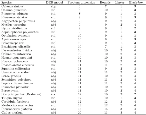
A total of 30 constrained DEB problems was considered, corresponding to different species, different models and different dimensions (see Table 2), reflecting the features of the complete collection of DEB problems to be solved (which comprises 1012 instances).
The Nelder-Mead Simplex algorithm with and without restarts, available in
the DEB toolbox, was tested against SID-PSM, an algorithm by Custodio and Vicente (2007) which corresponds to an implementation of a Directional Direct-Search method.
In SID-PSM (version 1.3), the search step is based on the minimization of quadratic polynomial interpolation or regression models of the objective func-tion, built by reusing function evaluations as proposed by Custodio et al. (2010) As positive spanning sets, to be used in the poll step, it was considered the default option of SID-PSM, which includes coordinate directions, suited for bound constraints, enhanced with two random directions, generated in the unit sphere, to account for the black-box constraints. Initialization was pro-vided by the DEB collection.
As stopping criteria, in SID-PSM it was considered a minimum step size of 10−4 or a maximum of 2000n function evaluations, where n represents the problem dimension. Regarding the Nelder-Mead Simplex method, it was con-sidered ∆f un = 10−4, ∆simplex = 10−4 or a maximum of 2000n function
Table 2 Overview of the set of DEB problems
Species DEB model Problem dimension Bounds Linear Black-box
Calanus sinicus sbp 6 7 1 3
Channa punctata std 8 10 1 3
Pleuroxus aduncus std 8 9 1 3
Pleuroxus striatus std 8 9 1 3
Argopecten purpuratus abj 9 9 2 4
Mytilus trossulus abj 9 9 2 4
Hydra viridissima stf 9 9 1 2 Aspidiophorus polystictos std 9 9 1 3 Octolasion cyaneum std 10 9 1 3 Apatosaurus spec std 10 9 1 3 Balaeniceps rex std 10 9 1 3 Brachionus plicatilis std 10 7 1 3
Paracentrotus lividus abj 10 10 2 4
Callianira antarctica abj 10 10 2 4
Haematopus moquini std 10 10 2 3
Pisaster ochraceus abj 11 10 2 4
Phascolarctos cinereus stx 11 11 2 2
Squatina californica std 11 9 2 3
Uranoscopus scaber abj 11 11 2 4
Beroe gracilis abj 11 10 2 4
Schmidtea polychroa abj 11 11 2 4
Lepidochitona cinerea abj 11 11 2 4
Planorbis planorbis abj 11 10 2 4
Beroe ovata abj 11 10 2 4
Bos primigenius (Brahman) stx 12 10 2 2
Tiliqua rugosa std 12 10 1 3
Crepidula fornicata abj 12 12 2 4
Merluccius merluccius std 13 12 2 4
Pleuronectes platessa abj 15 15 3 4
Gadus morhua abj 20 13 3 4
aThe column ‘Bounds’ provides the number of bound constraints, the column ‘Linear’ represents the
number of linear constraints, and ‘Black-box’ corresponds to the number of black-box constraints.
evaluations. When using the restart approach, the maximum number of func-tions evaluafunc-tions was distributed by 10 runs, with a maximum value of 200n functions evaluations per run.
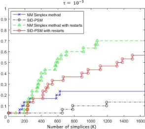
For reporting the results, we considered data profiles introduced by More and Wild (2009) which are widely used as tool for benchmark derivative-free optimization solvers.
A data profile provides a graphical representation of the percentage of prob-lems solved by a method for a given accuracy (τ ) versus the number of simplices (K) used, which corresponds to the quotient between the number of function evaluations required and the problem dimension plus one (n + 1). A problem is considered solved to the accuracy (τ ) if the following condition is satisfied:
f (x0) − f (x) ≥ (1 − τ )(f (x0) − fL), (9)
where τ > 0, x0 represents the initialization, and fL is computed for each
levels 10−2, 10−3, and 10−4 were considered in the analysis. Since the results were similar, we are only reporting for τ = 10−3.
Fig. 4 Data profile for the Nelder-Mead Simplex and SID-PSM algorithms, with and with-out the restart approach, for an accuracy level τ = 10−3.
Figure 4 corresponds to the data profile that compares the Nelder-Mead Simplex method without and with the restart procedure and the SID-PSM algorithm, considering an accuracy level τ = 10−3. It is clear the advantage of the simplex variants over SID-PSM, in particular when the restart proce-dure is applied, even for budgets of moderate size. The restart strategy seems to avoid the stagnation of the Nelder-Mead Simplex algorithm, allowing the exploitation of others areas of the variable space, conducting to better final solutions.
Based on these results, the restart approach was also applied to SID-PSM in an attempt of improving the corresponding performance. The result corre-sponds to the red line in Figure 4, which corroborates the value of the restart approach, clearly improving the results obtained with SID-PSM. Although, SID-PSM continues to not be competitive with the Nelder-Mead Simplex with restarts. Nevertheless, SID-PSM presents a well-established convergence anal-ysis, which is not the case for the variant of the Nelder-Mead Simplex method tested.
6 Simplex Directional Direct-Search (SimDDS)
The structure of each iteration of a Directional Direct-Search algorithm, or-ganized in a search step and a poll step, provides a natural framework for hybridizing the Nelder-Mead Simplex method with Directional Direct-Search.
Implementing a search step based on the Nelder-Mead Simplex algorithm will allow to take advantage of its good numerical performance, not jeopardizing the converge properties of Directional Direct-Search, since they result from the poll step.
Several hybrid versions of the two methods were considered, mainly differ-ing in the criteria adopted to define the search step as unsuccessful, interrupt-ing the simplex search and performinterrupt-ing the poll step. Only two will be reported, namely the ones that were more promising.
In the first hybrid version, the search step is considered unsuccessful when the difference between the objective function values at the simplex vertices reaches a given small threshold, which could mean that the algorithm reached a flat region, being adequate to check for stationarity by doing a local search around the best simplex vertex, using the poll step. The search step is also declared as unsuccessful when a maximum fixed number of function evalua-tions is attained or when the relative size of the simplex becomes smaller than a chosen tolerance ∆simplex> 0.
In the second hybrid version, additionally to the previous described criteria, no simplex shrinks are allowed, moving the algorithm to the poll step. When a shrink operation should be performed by the Nelder-Mead Simplex method, there is an indication that the algorithm is in stagnation, unable to proceed. A poll step around the best simplex vertex could indicate if stationarity has been reached.
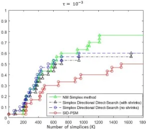
Fig. 5 Data profile for two hybrid variants of the Nelder-Mead Simplex and SID-PSM algorithms (Simplex Directional Direct-Search), for the Nelder-Mead Simplex method and for SID-PSM. The last two algorithms were applied using the restart approach.
Figure 5 corresponds to the data profile comparing the two hybrid ver-sions with the Nelder-Mead Simplex and SID-PSM algorithms. The last two algorithms considered the restart approach.
Both hybrid versions present a better performance than SID-PSM. How-ever, for larger budgets of function evaluations, these versions are not compet-itive with the Nelder-Mead Simplex algorithm. Nevertheless, as it was already pointed out, from all the solvers represented in the data profile of Figure 5, the Nelder-Mead Simplex algorithm is the only one without a well-established convergence analysis.
7 Strategies for constrained optimization in simplicial search Considering the techniques described in Section 3, there is not a clear indi-cation on how to address constraints when using the Nelder-Mead Simplex algorithm. Three different strategies were implemented, in an attempt of over-coming the consequences of the use of an extreme barrier function.
In fact, the strategies tested suggest additional function evaluations, al-lowing the exploitation of the feasible region near to the boundary, when the reflection operation is infeasible and the simplex needs to reduce its dimensions and volume.
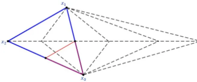
The first approach is motivated by Guin (1968) . When the reflected point is infeasible, a backtracking line-search approach moves it in the direction of the centroid until feasibility is reached. Figure 6 represents the application of this strategy in a two dimensions constrained problem, where f (x1) < f (x2) <
f (x3) and Ω represents a portion of the feasible region, nearby the current
simplex.
Fig. 6 Backtracking line-search strategy for constrained optimization with the Nelder-Mead Simplex method.
Since xr is infeasible, a backtracking procedure is initialized, towards x3,
by considering:
xBk= x3+ αk(xr− x3), with αk∈ ]0, 1[ (10)
and αk+1< αk. Points xB1 and xB2 are two of the resulting trial points. The
procedure stops once that feasibility is reached. If f (xBk) < f (x3) than xBk
is accepted as a vertex of the new simplex and the iteration ends. Otherwise, an inside contraction is performed.
The second approach is represented in Figure 7 and consists on an ad-ditional outside contraction, when the trial point obtained by reflection (xr)
is infeasible and the point computed in a following inside contraction is not accepted, f (xic) ≥ f (x3). In a regular iteration of the Nelder-Mead Simplex
method a shrink operation would be performed. As consequence, the size of the simplex would decrease, which could lead to the stagnation of the algorithm. The execution of an outside contraction before the shrink operation, allows the exploitation of the subspace near to the boundary of the feasible region and, if successful, avoids the decrease of the simplex size. If f (xoc) < f (x3),
then xoc is accepted as a vertex of the new simplex and the iteration ends.
Otherwise, the method performs the shrink operation.
Fig. 7 Additional outside contraction for constrained optimization with the Nelder-Mead Simplex method.
The third approach is similar to the second one but, in case of infeasibility of the reflected point, performs both the inside contraction and the outside contraction, choosing the trial point with the best objective function value.
So, if f (xic) ≤ f (xoc) and f (xic) < f (x3) , then xic is accepted as a
vertex of the new simplex and the iteration ends. If f (xic) > f (xoc) and
f (xoc) < f (x3) , then the iteration ends and xoc is accepted as a vertex of
the new simplex. Otherwise, the method performs a shrink operation. The strategy is described in Figure 8.
Fig. 8 Best of inside-outside contractions for constrained optimization with the Nelder-Mead Simplex method.
The three proposed strategies were implemented in the Nelder-Mead Sim-plex algorithm with the restart approach. Figure 9 provides the corresponding data profile.
Fig. 9 Data profile for the three variants for handling constraints applied to the Nelder-Mead Simplex algorithm with the restart approach.
Based on the numerical results obtained, there is not a clear indication of the value of any of the strategies to improve the numerical efficiency of the algorithm. In fact, the results obtained are similar to the ones corresponding to the Nelder-Mead Simplex method only considering the restart approach.
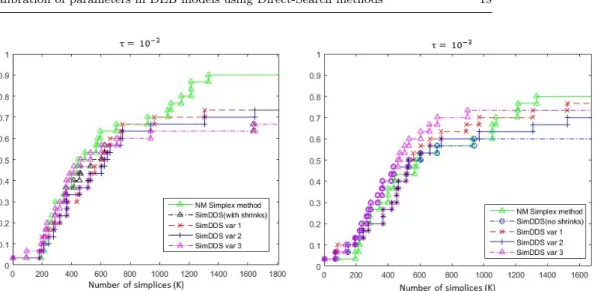
Anyway, the three developed variants were also applied to the hybrid Sim-plex Directional Direct-Search algorithm. The corresponding results are re-ported in Figures 10 a) and 10 b), for the first and second hybrid versions, respectively.
From the analysis of these data profiles, it is possible to conclude that the application of the strategies to handle constraints improved the performance of the Simplex Directional Direct-Search algorithm, in particular in the case of the second variant, where the shrink operation is not performed. The im-provement is more pronounced when considering the third strategy to address constraints, where it is possible to choose between the best of the inside and outside contraction operations.
8 Conclusions
This work accessed the numerical performance of the Nelder-Mead Simplex algorithm, implemented in the DEB toolbox, when calibrating parameters in DEB models, by comparison with Directional Direct-Search. The Nelder-Mead
(a) Results for the Simplex Directional Direct-Search algorithm, allowing shrinks.
(b) Results for the Simplex Directional Direct-Search algorithm, without the shrinking operation.
Fig. 10 Comparison between the results obtained with the Nelder-Mead Simplex algorithm with restarts, the two variants of Simplex Directional Direct-Search (SimDDS), and the application of the different strate-gies to address constraints to SimDDS.
Simplex method with restarts proved its competitiveness, although it does not provide guarantees of convergence.
The good numerical performance of the restart approach is not specific of its joint application with the Nelder-Mead Simplex algorithm. This strategy can be used to improve the numerical performance of other classes of methods. Compelling results were obtained with the SID-PSM algorithm.
The development of a hybrid version of Simplex Search and Directional Direct-Search, incorporating strategies to address constraints, allowed to re-tain the convergence properties of Directional Direct-Search and the good numerical performance of the Nelder-Mead Simplex method with restarts.
Recently, the authors were aware of another hybrid variant of these two classes of optimization methods, developed in parallel with the current work by Audet and Tribes (2018) . While there are some similarities between the two approaches, since the Nelder-Mead Simplex algorithm is also used to define a search step in a Directional Direct-Search method, with similar conditions to define the search step as unsuccessful, constraints are addressed with a filter technique, which would not be possible in the context of the estimation of DEB models parameters.
In future, the Simplex Directional Direct-Search, without the shrinking op-eration and with the variant of choice between the inside-outside contractions for addressing infeasibility, will be implemented in the DEB toolbox and ap-plied to the complete Add-my-Pet collection. A comparison between the model parameters computed with the new procedure and the current estimated
pa-rameters, recorded in the collection, will allow to access the corresponding biological contribution of the proposed method.
Finally, we note that the new algorithmic framework of Simplex Directional Direct-Search is not specific of being applied to DEB optimization problems. Rather, it can be applied to any general derivative-free constrained optimiza-tion problems, where infeasible points can not be evaluated, being a valuable tool in several domains of simulation-based optimization.
References
1. Add-my-Pet collection (2018). http://www.bio.vu.nl/thb/deb/deblab/add my pet 2. Audet C, Dennis J (2003) Analysis of generalized pattern searches. SIAM J Optimiz
13:889–903
3. Audet C, Dennis J (2006) Mesh adaptive direct search algorithms for constrained opti-mization. SIAM J Optimiz 17:188–217
4. Audet C, Tribes C (2018) Mesh-based Nelder-Mead algorithm for inequality constrained optimization. Comput Optim Appl. doi: 10.1007/s10589-018-0016-0
5. Baas J, Augustine S, Marques GM, Dorne J-L (2018) Dynamic energy budget models in ecological risk assessment: From principles to applications. Sci Total Environ 628–629:249– 260
6. Box MJ (1965) A new method of constrained optimization and a comparison with other methods. Comput J 8:42–52
7. Conn AR, Scheinberg K, Vicente LN (2009) Introduction to Derivative-Free Optimiza-tion. MPS-SIAM Series on OptimizaOptimiza-tion. SIAM, Philadelphia
8. Cust´odio AL, Rocha H, Vicente LN (2010) Incorporating minimum Frobenius norm models in direct search. Comput Optim Appl 46:265–278
9. Cust´odio AL, Vicente LN (2007) Using sampling and simplex derivatives in pattern search methods. SIAM J Optimiz 18:537–555
10. Fan E (2002) Global Optimization of Lennard-Jones Atomic Clusters. Master Thesis, McMaster University, Hamilton, Canada
11. Fletcher R, Leyffer S (2002) Nonlinear programming without a penalty function. Math Program 91:239–269
12. Guin J (1968) Modification of the complex method of constrained optimization. Comput J 10:416–417
13. Hare WL (2010) Using derivative free optimization for constrained parameter selection in a home and community care forecasting model. In: International Perspectives on Oper-ations Research and Health Care, Proceedings of the 34th Meeting of the EURO Working Group on Operational Research Applied to Health Sciences, pp 61–73
14. Jager T, Barsi A, Hamda NT, Martin BT, Zimmer EI, Ducrot V (2014) Dynamic energy budgets in population ecotoxicology: Applications and outlook. Ecol Model 280:140–147 15. Kelley CT (1999) Detection and remediation of stagnation in the Nelder-Mead algorithm
using a sufficient decrease condition. SIAM J Optimiz 10:43–55 16. Kleiber M (1932) Body size and metabolism. Hilgardia 6:315–353
17. Kolda TG, Lewis RM, Torczon V (2003) Optimization by direct-search: New perspec-tives on some classical and modern methods. SIAM Rev 45:385–482
18. Kooijman SALM (1986) Energy budgets can explain body size relations. J Theor Biol 121:269–282
19. Kooijman SALM (2000) Dynamic Energy and Mass Budgets in Biological Systems. Cambridge University Press
20. Kooijman SALM (2010) Dynamic Energy Budget Theory for Metabolic Organisation. Cambridge University Press
21. Kooijman SALM (2011) Basic Methods in Theoretical Biology. Part of the DEB tele-course, Vrije Universiteit, Amsterdam
22. Lagarias JC, Reeds JA, Wright MH, Wright PE (1998) Convergence properties of the Nelder-Mead simplex method in low dimensions. SIAM J Optimiz 9:112–147
23. Le Floc’h F (2012) Issues of Nelder-Mead simplex optimisation with constraints. SSRN eLibrary, 2097904
24. Lewis RM, Torczon V (2000) Pattern search methods for linearly constrained minimiza-tion. SIAM J Optimiz 10:917–941
25. Lika K, Kearney MR, Kooijman SALM (2011) The “covariation method” for estimat-ing the parameters of the standard Dynamic Energy Budget model II: Properties and preliminary patterns. J Sea Res 66:278–288
26. Marques GM, Lika K, Augustine S, Pecquerie L, Kooijman S (2018) Fitting multiple models to multiple data sets. J Sea Res. doi: 10.1016/j.seares.2018.07.004
27. McKinnon KIM (1998) Convergence of the Nelder-Mead simplex method to a nonsta-tionary point. SIAM J Optimiz 9:148–158
28. Mor´e JJ, Wild SM (2009) Benchmarking derivative-free optimization algorithms. SIAM J Optimiz 20:172–191
29. Nelder JA, Mead R (1965) A simplex method for function minimization. Comput J 7:308–313
30. Nisbet RM, Muller EB, Lika K, Kooijman SALM (2000) From molecules to ecosystems through dynamic energy budget models. J Anim Ecol 69:913–926
31. Nocedal J, Wright SJ (2006) Numerical Optimization. Springer-Verlag, second edition 32. Price CJ, Coope ID, Byatt D (2002) A convergent variant of the Nelder-Mead algorithm.
J Optimiz Theory App 113:5–19
33. Sousa T, Domingos T, Kooijman SALM (2008) From empirical patterns to theory: a formal metabolic theory of life. Philos T Roy Soc B 363:2453–2464
34. Sousa T, Domingos T, Poggiale JC, Kooijman SALM (2010) Dynamic Energy Budget theory restores coherence in biology. Philos T Roy Soc B 365:3413–3428
35. Torczon V (1997) On the convergence of pattern search algorithms. SIAM J Optimiz 7:1–25
36. Tseng P (1999) Fortified-descent simplicial search method: A general approach. SIAM J Optimiz 10:269–288
37. van der Meer J (2006) An introduction to Dynamic Energy Budget (DEB) models with special emphasis on parameter estimation. J Sea Res 56:85–102
38. Vicente LN, Cust´odio AL (2012) Analysis of direct searches for discontinuous functions. Math Program 133:299–325
39. von Bertalanffy L (1957) Quantitative laws in metabolism and growth. Q Rev Biol 32:217–231