PARAMETERS ESTIMATION IN THE MODEL FOR IN SITU DEGRADABILITY OF MERTENS AND LOFTEN

MUNIZ, J. A. et al.

1622

PARAMETERS ESTIMATION IN THE MODEL FOR

IN SITU

DEGRADABILITY

OF MERTENS AND LOFTEN

1

Estimação dos parâmetros no modelo para degradabilidade in situ de Mertens e Loften

Joel Augusto Muniz2_{, Taciana Villela Savian}3_{, João Domingos Scalon}4

ABSTRACT

The aim of this study is to evaluate the behavior of the parameters of the degradation model proposed by Mertens & Loften (1980) fitted to the results of a rehearsal of degradability in situ. In the experiment, we evaluate the potentially degradable residue of neutral detergent fiber (NDF) of coastcross grass (Cynodon dactylon x Cynodon nlemfunensis) cut at 60 days, with three replications. The potentially degradable residue of NDF is studied using fifteen incubation times (0; 0.5; 1; 3; 6; 9; 12; 18; 24; 36; 48; 56; 72; 96 and 120 hours). The experimental plot is comprised of a non-lactating cow with a permanent ruminal fistula. It is obtained mean and individual fits for the animals. Variances of parameter estimators is also obtained through both the covariance matrix of the parameters and the jackknife method, then resulting expressions for the estimate of the confidence interval for the parameters of the model. The results shows that the jackknife method presents larger variance estimate for the parameters of the model of Mertens & Loften (1980), resulting in confidence intervals of greater amplitude and less precise parameter estimates for both the individual and mean fits.

Index terms: Nonlinear regression, ruminal degradability, jackknife method, coast-cross grass.

RESUMO

Objetiva-se avaliar o comportamento dos parâmetros do modelo de degradação proposto por Mertens & Loften (1980) ajustado aos resultados de um ensaio de degradabilidade in situ. No experimento é avaliado o resíduo potencialmente degradável da fibra em detergente neutro (FDN) da gramínea coastcross (Cynodon dactylon x Cynodon nlemfunensis) cortada aos 60 dias, com três repetições. O resíduo potencialmente degradável da FDN é estudado utilizando quinze tempos de incubação (0; 0,5; 1; 3; 6; 9; 12; 18; 24; 36; 48; 56; 72; 96 e 120 horas). A parcela experimental é constituída por uma vaca não lactante, com fístula ruminal permanente. São obtidos ajustes médios e individuais para os animais. Obtem-se também as variâncias dos estimadores dos parâmetros por meio da matriz de variância e covariância dos parâmetros e pelo método jackknife, propondo-se expressões para a estimação do intervalo de confiança para os parâmetros do modelo. Os resultados mostram que o método de jackknifeapresenta maior estimativa de variância para os parâmetros do modelo de Mertens & Loften (1980), resultando em intervalos de confiança de maior amplitude e estimativas dos parâmetros menos precisas, nos ajustes individuais e médios.

Termos para indexação: Regressão não-linear, degradabilidade ruminal, método jackknife, gramínea coastcross.

(Received in april 27, 2006 and approved in april 2, 2007)

1_{Trabalho conduzido com apoio do CNPq.}

2_{Engenheiro Agrônomo, Doutor, Professor Titular Departamento de Ciências Exatas/DEX Universidade Federal de Lavras/UFLA Cx. P. 3037} 37200-000 Lavras, MG joamuniz@ufla.br

3_{Zootecnista, Mestre em Estatística e Experimentação Agropecuária Departamento de Ciências Exatas/DEX Universidade Federal de Lavras/UFLA} Cx. P. 3037 37200-000 Lavras, MG tacianavillela@gmail.com

4_{Estatístico, PhD, Professor Associado Departamento de Ciências Exatas/DEX Universidade Federal de Lavras/UFLA Cx. P. 3037 37200-000} Lavras, MG scalon@ufla.br

INTRODUCTION

Quantitatively, carbohydrates are the most important nutrients in the diet of ruminants. Vegetables contain approximately 75% of these elements that are the primary source of energy for the microorganisms of the rumen and for the host animal. The main carbohydrates found in the vegetables are cellulose, hemicelulose, pectins, fructosans, and starch. The microorganisms of the rumen present high capacity of utilization of these carbohydrates, in that the ruminants use the final products of the ruminal fermentation, more specifically the fatty acids that are absorbed, supplying most of the energy demands of the animals.

For a long time, the feeding of ruminants was inadequate, because it was just based on the amount, and not on the quality of the feeds. Today, the characterization of feeds according to their chemical composition, and the constitution of their different fractions, degraded or not, in the rumen, is one of the principal objectives of nutritionists when balancing rations that provide nutrients for the growth and development of the microorganisms in the rumen and, consequently, of the animal.

Parameters estimation in the model... 1623 that remains packed in nylon bag, in different periods of

time. This technique was already known in 1930, when Quinn et al. (1938) used this method to evaluate the digestion of the feedstuff in the rumen of fistulated sheeps. According to Mertens (1993), the first evaluations of digestion processes and conversion, those depended on retention times, were qualitative and based on the visual interpretation of digestion curves. The description of the process was difficult because the digestion curves showed nonlinear behavior, and seemed to not fit to the kinetics of typical chemical reactions. According to Mertens (1993), Waldo, in 1970, was the first to report that degradation profiles were combinations of digestible and indigestible material, and that the potentially digestible fraction would follow kinetics of first order. Mertens (1977) verified that the digestion of the neutral detergent fiber (NDF) presented a period in that degradation of the component indeed didn t happen. Mertens & Loften (1980) suggested the inclusion of a parameter, for the estimates of the parameters of the model of first order of Waldo et al. (1972) that contemplated this period for degradability in vitro and in situ of NDF, dry matter (DM) and nitrogen (N).

Souza (1998) considers the nonlinear regression model in the form

y

_t

f x

( ,

_t 0

)

_t, where t = 1, ..., n;

0

( ,

_t

)

f x

h a s k n o w n fu n c tio n a l fo rm ;

x

_t is a k dimensional vector formed by observations in exogenous variables, 0 _{is a p dimensional parameter belonging} to the parametric space e _t is an experimental error,, not directly visible. The same author mentions that, in a similar way to linear models, the process of parameter estimates in a nonlinear model can be obtained by the minimization of the error sum of squares, obtaining the system of normal nonlinear equations, which does not present a closed-form solution for the parameter estimate, and therefore, it must be obtained by iterative processes. The success in the use of Gauss-Newton s algorithm, as an iterative method, will depend on the appropriate choice of both the function response and starting values. Although some general orientations exist for determination of starting values, the choice process is a procedure resolved by the researcher. Several alternatives for the determination of those values are presented in Draper & Smith (1998) and Gallant (1987).

Some important statistical considerations, usually ignored in the studies of the curves of ruminal degradation, are the heterogeneity of variances of the percentage of degradation of the food in time, and the existence of autocorrelation of the regression residuals. Violating the assumptions of homogeneity of variances and no autocorrelation, then the estimates are likely to be biased

and the variances of the parameters are subestimated, respectively. (SOUZA, 1998).

In agreement with Hoffman & Vieira (1998), in presence of heterogeneity of variances, the weighted least squares procedure is more appropriate for supplying unbiased estimators with minimum variance, while in the presence of both heterogeneity of variances and autocorrelation of the residuals, the generalized least squares method is more efficient than both weighted and ordinary least squares methods.

Usually, in basic regression models, it is assumed that the errors are not correlated, that is, that they are independent, which is not appropriate when one works with chronological series of data. In such a case, the error corresponding to an observation is correlated with the error of the previous observation (HOFFMANN & VIEIRA, 1998). According to Morettin & Toloi (2004), the general characteristic of the autocorrelation of the residuals is the one of a systematic variation of the values among successive observations. When this happens, it is said that the residuals present autocorrelation.

According to Mood et al. (1974), the deficiency observed in the point estimator is that by itself conveys no information about its closeness to the parameter value and, therefore, supply limited information regarding the parameters. In practice, only rarely the point estimate is exactly equal to the parameter. This situation makes possible the inference to be complemented, whenever possible, with presuppositions concerning the probabilities of being close or not to its point estimate. That can be done by the construction of confidence intervals so that, with a chosen degree of confidence (probability) the value of the parameter will be captured inside the interval. Several methods may exist for obtaining those intervals, though, the question is to determine which is the best interval. It is considered the more appropriate the one that presents minimum amplitude.

Vieira (1995) compared three statistical models, among them the one of Mertens & Loften (1980), for estimate of the kinetics of ruminal degradation in vitro and in situ of elephant grass (Pennisetum purpureum Schum. cv. Miner), cut at 61, 82, 103, 124, and 145 days after planting. Also, Feitosa (1999) used the same model to describe the degradation of the dry matter, crude protein, and NDF of coastcross grass hay.

MUNIZ, J. A. et al. 1624

The main aim of this work is to estimate the parameters of the degradability model of Mertens & Loften (1980) and to calculate the confidence intervals for the parameters by using both the covariance matrix of the parameters and the jackknife resampling method using data of an experiment of degradability in situ with fistulated cows.

MATERIAL AND METHODS

To illustrate the methodology, experimental data was used (REIS, 2000) of the potentially degradable residue, of the neutral detergent fiber (NDF), of coastcross grass (Cynodon dactylon x Cynodon nlemfunensis), cut at 60 days of age. The degradation profile was evaluated at fifteen incubation times (0; 0.5; 1; 3; 6; 9; 12; 18; 24; 36; 48; 56; 72; 96 and 120 hours), the experimental portion been constituted by a non-lactating cow, with a permanent ruminal fistula.

The model used to describe the potentially degradable residue was of Mertens & Loften (1980), given as:

( )

0

( ) D_{c t L}I para t L

R t

De I para t L

where R(t) is the residue after the incubation in the rumen in the time t (%); D is the degradable fraction (%); c is the degradation rate (%/h); t is the time of incubation (hours); I is the insoluble fraction and non-degradable (%) and L is the colonization time of the particles or lag time (hours).

This model is considered nonlinear and segmented, therefore the partial derivatives in relation to the parameters, for the larger times than the colonization time (t>L), continue in function of the parameters themselves, as shown by the following equations: R t( ) _ec t L( )

D

( )

( )

( ) c t L

R t

t L De c

( )

( ) c t L

R t cDe L

, R t( ) 1

I ,

Several iterative methods have been proposed in the literature for obtaining the least squares estimates of the parameters of a nonlinear regression model. One of them is Gauss-Newton s method that makes use of the partial derivatives, and consists of the development of Taylor series to the term of first order of the function

(

_i

, )

f X

around the point 0_.

The iterative formula known with Gauss-Newton s method is given by 1 0

(

X X

'

)

1

X e

'

, where X is the matrix of partial derivatives in relation to the parameters. This process is repeated placing 1 _{in the} place of 0_{(vector of starting estimates) until some}

convergence criterion is accepted. The speed in the

convergence depends on the complexity of the model in study and, mainly, on the quality of the starting values, necessary in any iterative method.

The matrix of partial derivatives (X) is of the type

nXp, being n the number of incubation times of the samples

in the rumen (n=15) and p the number of parameters of the model (p=4) and assumes the form X (am1am2 am3 am4)

where the elements of this matrix are vectors column of type 15x1, and m assumes the values of the incubation times, in other words, 0; 0,5; 1; 3; 6; 9; 12; 18; 24; 36; 48; 56; 72; 96, and 120.

If in the vectors column m L then, the partial derivatives are: 1 ( ) 1 m R t a D 2 ( ) 1 m R t a I , 3 ( ) 0 m R t a c e

If in the vectors column m>L then, the partial

derivatives are: ( )

1

( ) c t L m R t a e D 2 ( ) 1 m R t a I , ( ) 3 ( )

( ) c t L

m

R t

a t L De

c

( ) 4

( ) c t L

m

R t

a cDe

L e

In this case, X X is a symmetrical matrix (4×4) and its elements (b_ij) can be written in the following way,

15 2 ( ) 11

1

1 i

L n

c t L

i i L

b e 15 ( ) 12 21 1 1 i L n

c t L

i i L

b b e

15

2 ( )

13 31 ( )

i

n

c t L i

i L

b b t L D e 15 2 ( )

14 41

i

n

c t L

i L

b b Dc e

22

b n

15

( )

23 32 ( )

i

n

c t L i

i L

b b t L D e

15

( ) 24 42

i

n

c t L

i L

b b Dc e

15

2 2 2 ( ) 33 ( )

i

n

c t L i

i L

b t L D e

15

2 ( ) 2

34 43 ( )

i

n

c t L i

i L

b b t L D c e 15 2 2 2 ( ) 44

i

n

c t L

i L

b D c e

where is the greatest integer function, in other words,

x

is the greatest integer not superior to x.

Draper & Smith (1998) present the estimates of the asymptotic matrix of covariances in the following manner:

1 1 2 1

1 2 1 2 2

1 2 ( , ) ( , ) ( , ) ( , ) ' ( , ) ( , ) j j

j j j

V Cov Cov

Cov V Cov

V X X QME

Parameters estimation in the model... 1625 with j = 1,..., p, where p is the number of parameters.

In this manner, the confidence interval is defined for the parameter as

, ₂

j j _{n p} j

IC t V , where _j

is the estimate of the j-th parameter, , 2

n p

t _{is the}

superior percentile ₂ of the Student s t-distribution with n-p degrees of freedom and V j is the estimate of the

standard error of the estimate of the j-th parameter. Since there are no closed-form expressions for the variance estimators of the parameters of the model in study, the jackknife resampling method is also used to build the confidence intervals for the parameter estimates of the model of Mertens & Loften (1980), Those intervals are obtained in the following way: first, the estimates of the parameters is obtained, through the SAS program (1995), by using the data set without the first incubation time. Soon after, the process is repeated considering the original data set without the second incubation time and, successively, until all the partial jackknife estimates have been calculated. This process allowed to obtain a group of 15 partial estimates of the parameters. The estimates were applied to the following formula: * * *

1

j j

E nE n E ,

with j = 1,..., 15, where

E

*_j is the estimate of the pseudo-value for the parameter when the j-th incubation time was excluded, n is the number of observations, *

E

is the estimate of the parameters with all the incubation times and

E

*_j is the value of the partial parameter estimate obtained by the fitted model by using the SAS program (1995) when the j-th incubation time was excluded. Then, the mean ( *

E

) was obtained, which represents the jackknife estimator and the variance of this estimator in a conventional way, making possible the construction of the confidence interval as follows: *

100(1 )% _1,

2

n

S

IC E t

n

where 1, 2

n

t _{is the superior percentile}

2 of the Student s t-distribution with n-1 degrees of freedom, and S is the standard deviation of the pseudo-values

E

*_j.

Parameter estimates were obtained for both the individual curves and the average curve of the model in question. To verify the heterogeneity of variances, the variance of the potentially degradable residues was calculated for each incubation time, making possible the calculation of maximum F of Hartley (PEARSON & HARTLEY, 1970), obtained by the quotient between the maximum and minimum residual variance, in that the non-significance shows that there is no heterogeneity of variances. To verify the presence of residual auto-correlation it was used both the macro %AR (y, p), implemented in the proc model (SAS, 1995) and the correlogram analysis.

RESULTS AND DISCUSSION

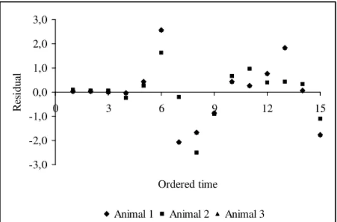
Just as in linear regression analysis, it is extremely important in nonlinear regression to have tools that allow goodness-of-fit of the model in a given application. The typical representations of informal diagnosis in nonlinear regression involve the plots of residuals against the independent variables (or ordered sequence) to check for nonconstant variance (heterocedasticity), influential observations and specification errors in the response function.

Figure 1 shows the plot of the residuals against the ordered sequence of the independent variable (incubation times), for the individual fits of the animals. It is noticed that the plot of residuals, for grass cut at 60 days, does not demonstrate evidences of any heterocedasticity pattern. A typical heterocedasticity pattern that can be found is mentioned by Vieira (1995), whereas the evaluation of the model of Mertens & Loften (1980) linearized for logarithmic transformation, tended to present the band of residuals widening to the right (larger times) showing nonconstant variance.

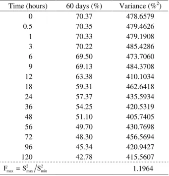
Table 1 shows the values of mean degradation of NDF (in percentage) and their variances. It is observed that, with the increase of the incubation time of the samples in the rumen, there is a decrease in the residual variances of the degradation of NDF of coastcross grass. The relationship between the maximum and the minimum variance is of 1.20 for the cut of the grass at 60 days, not showing the presence of heterogeneity. In other words, this relationship is not significant for 3 experimental groups (3 animals) and 14 degrees of freedom, with a significance level of 5%, according to the Hartley s maximum F test.

The ratio between the maximum and minimum. variance was also used by Mazzini (2001) when studying

Figure 1 Plot of residuals versus ordered time, for each animal, with regards to grass cut at 60 days.

-3,0 -2,0 -1,0 0,0 1,0 2,0 3,0

0 3 6 9 12 15

Ordered time

R

es

id

u

al

MUNIZ, J. A. et al. 1626

growth curves of bovines of the Hereford breed. This author tells us that, as the age of the animals increased, there is an increment in the variances of the body weights. This may be also a possible source of heterocedasticity pattern.

It is observed in Table 2 that the autocorrelation parameters ( ₁ and ₂) are not significant at a significance level of 5%, then not being necessary the fit of autoregressive structure errors. Mazzini (2001), Mazzini et al. (2003) and Mazzini et al. (2005), when studying growth curves of bovine through several functions considering autocorrelation of the residues, found that some functions didn t fit to an autoregressive model of 1st or 2nd order when fitting mean curves; however, when fitting individual curves there were animals that presented these error structures.

Table 1 Observed mean values of the potentially degradable residue (PDR) of NDF (%) per incubation time and its respective variances.

Time (hours) 60 days (%) Variance (%2)

0 70.37 478.6579

0.5 70.35 479.4626

1 70.33 479.1908

3 70.22 485.4286

6 69.50 473.7060

9 69.13 484.3708

12 63.38 410.1034

18 59.31 462.6418

24 57.37 435.5934

36 54.25 420.5319

48 51.10 405.7405

56 49.70 430.7698

72 48.30 456.5694

96 45.34 420.9427

120 42.78 415.5607

2 2 max max min

F = S S 1.1964

Table 3 shows the parameter estimates of the model of Mertens & Loften (1980) without considering the structure of correlated errors (they were not necessary) with the respective variance estimates obtained by both the covariance matrix of the parameters and the jackknife method.

Regarding to the parameter estimate values, Feitosa (1999), studying the comparison of models in rehearsals of degradability in situ with coastcross grass hay, observed

that the model of McDonald (1981), also corrected for the colonization time, resulted in the same estimates for the model of Mertens & Loften (1980). This author reports values of 43.26% for insoluble and non-degradable fraction; 4.4%h-1 _{for the degradation rate (parameter c) and}

2.45 hours for the time of colonization. This model was also used by Lira (2000) to predict the degradation of NDF of braquiaria grass (Brachiaria decumbens Stapf.), during two seasons (dry and rainy), finding mean values of 51.32% for the degradable fraction; 38.08% for the insoluble and non-degradable fraction; 2.5%h-1 _{for the degradation rate}

(parameter c) and 7.64 hours for the colonization time, during the rainy season.

Table 2 Descriptive level of the autocorrelation parameter tests for the individual and mean fits, for grass cut at 60 days, considering a structure of first and second order autoregressive errors.

The parameter estimate values obtained by the jackknife method didn t suffer great alterations. Whereas, the variance estimates of the parameter estimates, obtained by this method presented significant increases in its values, resulting in confidence intervals of greater amplitude, and less precise parameter estimates.

This increase in the variance estimate of the parameter estimates, when compared with the estimates obtained by the covariance matrix of the parameters, can be explained by the fact that when excluding the j-th sample observation, the program converged for values differing of the partial estimates, affecting directly the estimate of the pseudo-value of the parameter directly and its variance.

This methodology was also used by Pereira et al. (2005) when studying the prediction of the nitrogen mineralized in Latossolo through nonlinear models. When comparing confidence intervals obtained by using the covariance matrix of the parameters and by using the jackknife method, the authors also verified that this second method provided greater variance estimates of the parameters.

AR (1) AR (2)

Individual

and mean fits _{1 1 2}

Animal 1 0.7527 0.6799 0.2946

Animal 2 0.4165 0.0750 0.0628

Animal 3 0.7538 0.6814 0.2949

Parameters estimation in the model... 1627 Table 3 Parameter estimates and variance estimates of the parameter obtained by the covariance matrix of the parameters and for the jackknife method, respectively.

Covariance Matrix Jackknife

Parameters _{V LL}1

UL1 _V LL1 UL1

D 27.3689 2.2678 24.0547 30.6831 27.3309 87.1121 22.7310 33.0690 I 52.5959 1.7727 49.6657 55.5261 52.6347 86.9331 46.8880 57.2170 C 0.0318 2.35x10-5 0.0211 0.0425 0.0320 0.0012 0.0096 0.0476

A

n

im

al

1

L 4.4316 2.3249 1.0759 7.7873 4.4203 64.8300 0.1309 9.0496

D 25.5985 1.6552 22.7671 28.4299 25.5569 59.5559 21.9076 30.4558 I 19.6292 1.3608 17.0619 22.1965 19.6292 59.0303 14.8556 23.3659 C 0.0284 1.41x10-5 0.0201 0.0367 0.0284 0.0006 0.0120 0.0399

A

n

im

al

2

L 4.7424 1.8198 1.7735 7.7113 4.7424 36.5709 1.5020 8.2005

D 27.3698 2.2701 24.0539 30.6857 27.3301 87.1015 22.7578 33.0955 I 58.4006 1.7748 55.4686 61.3325 58.4413 86.9509 52.6671 62.9958 C 0.0318 2.35x10-5 0.0213 0.0425 0.0320 0.0016 0.0095 0.0475

A

n

im

al

3

L 4.4305 2.3274 1.0729 7.7880 4.4206 64.7665 0.1119 9.0263

D 26.7738 1.8948 23.7444 29.8032 26.7406 78.4343 22.3336 32.1435 I 43.5473 1.5066 40.8459 46.2486 43.5828 77.9835 38.1595 47.9412 C 0.0306 1.84x10-5 0.0211 0.0400 0.0308 0.0009 0.0105 0.0453

M

ea

n

F

it

L 4.5118 1.9970 1.4017 7.6218 4.4928 60.8839 0.4549 9.0979

1-LL (lower limit), UL (upper limit.

CONCLUSIONS

The model of Mertens & Loften (1980) was adapted to describe the degradability in situ of neutral detergent fiber of coastcross grass (Cynodon dactylon x Cynodon nlemfunensis).

The jackknife method provided greater variance for the parameter estimates of the model of Mertens & Loften (1980), resulting in confidence interval of greater amplitude and less precise parameter estimates in both individual and mean fits.

REFERENCES

DRAPER, N. R.; SMITH, H. Applied regression analysis.

New York: J. Wiley & Sons, 1998. 706p.

FEITOSA, J. V. Ensaios de degradabilidade in situ:uma

abordagem estatística. 1999. 117p. Dissertação (Mestrado

em Zootecnia)-Universidade de São Paulo, Jaboticabal, 1999. GALLANT, A. R. Nonlinear statistical models. New York: J. Wiley, 1987. 610 p.

HOFFMANN, R.; VIEIRA, S. Análise de regressão: uma

introdução à econometria. São Paulo: HUCITEC, 1998. 379p.

LIRA, V. M. C. Utilização de diferentes modelos matemáticos e marcadores para simulação da cinética

digestiva e de trânsito do capim braquiária (Brachiaria

decumbens Stapf.). 2000. 90p. Dissertação (Mestrado em Zootecnia)-Universidade Federal de Viçosa, Viçosa, 2000. MAZZINI, A. R. de A. Análise da curva de crescimento de machos Hereford considerando heterogeneidade de

variâncias e autocorrelação dos erros. 2001. 94p.

Dissertação (Mestrado em Estatística e Experimentação Agropecuária)-Universidade Federal de Lavras, Lavras, 2001.

MAZZINI, A. R. de A. et al. Análise da curva de crescimento de machos Hereford. Ciência e Agrotecnologia. Lavras, v.27, n.5, p.1105-1112. 2003.

MAZZINI, A. R. de A. et al. Curva de crescimento de novilhos Hereford: heterocedasticidade e resíduos autoregressivos. Ciência Rural. Santa Maria, v.35, n.2, p.422-427. 2005.

McDONALD, I. A revised model for the estimation of protein degradability in the rumen. Journal of Agricultural

Science, v.96, p.251-252.1981.

MUNIZ, J. A. et al. 1628

MERTENS, D. R. Rate and extent of digestion. In: FORBES, J. M.; FRANCE, J. (Ed.) Qualitative aspects of ruminant

digestion and metabolism. Wallingford, UK: Cambridge

University, 1993. Cap. 2, p.13-51.

MERTENS, D. R.; LOFTEN, J. R. the effects of starch on forage fiber digestion kinetics in vitro. Journal of Dairy

Science, v.63, p.1437-46. 1980.

MOOD, A. M; GRAYBILL, F. A; BOES, D. C. Introduction

to the theory of statistics. Tokyo: McGraw-Hill Kogakusha,

1974. 564 p

MORETTIN, P. A.; TOLOI, C. M. de C. Previsão de séries

temporais. São Paulo: Atual, 2004. 436p.

PEARSON, E. S.; HARTLEY, H. O. Biometrika tables for

statisticians. Cambridge: Cambridge University, 1970. v.1.

PEREIRA, J. M. et al. Non linear models to predict nitrogen mineralization in an oxisol. Scientia Agrícola, v.62, n.4, p.395-400, 2005.

QUINN, J. I.; VAN DER WATH, J. G.; MYBURGH, S. Studies on the alimentary tract of merino sheep in South Africa.

Description of experimental technique. Journal of

VeterinaryScience Animal Indian, Ondersteport, v.11, n.2,

p.341-360, 1938.

REIS, S. T. dos. Valor nutricional de gramíneas tropicais

em diferentes idades de corte. 2000. 99p. Dissertação

(Mestrado em Zootecnia)-Universidade Federal de Lavras, Lavras, 2000.

SAS INSTITUTE Inc. SAS/ETS® _{User s Guide. Version 6.}

2.ed. Cary, 1995.

SOUZA, G. da S. Introdução aos modelos de regressão

linear e não-linear. Brasília: Embrapa-SPI/Embrapa-SEA,

1998. 489p.

VIEIRA, R.A.M. Modelos matemáticos para estimativa de parâmetros da cinética de degradação do capim elefante (Pennisetum purpureum, Schum., cv. Mineiro) em

diferentes idades de corte. 1995. 88p. Dissertação (Mestrado