Accretion versus outflow regions around Young Stellar Objects

D

Accretion versus

outflow regions

around Young

Stellar Objects

Raquel Maria Galhofa de Albuquerque

Programa Doutoral em Astronomia

Departamento de Física e Astronomia 2020

Orientadores

João José de Faria Graça Afonso Lima,

Professor auxiliar, Faculdade de Ciências da Universidade do Porto Jorge Filipe da Silva Gameiro

Professor auxiliar, Faculdade de Ciências da Universidade do Porto Christophe Sauty

around Young Stellar Objects

PhD Thesis co-supervised between the University of Porto and Observatoire de Paris

Raquel Maria Galhofa de Albuquerque

Departamento de Física e Astronomia, Faculdade de Ciências, Universidade do Porto Instituto de Astrofísica e Ciências do Espaço, CAUP

Laboratoire Univers et Théories, Observatoire de Paris, Université PSL, CNRS, Université de Paris

Advisors João J. G. Lima Jorge F. Gameiro Christophe Sauty

Dissertation submitted to the University of Porto for the degree of Doctor of Philosophy in Astronomy and to the Observatoire de Paris for the degree of Doctorat en Astronomie

et Astrophysique

Firstly, I am deeply thankful to my supervisors Christophe Sauty, Filipe Gameiro and João Lima for all their guidance, discussions, scientific insight and support throughout these last years. Without them this PhD would not be possible.

I would also like to express my gratitude to Fundação para a Ciência e a Tecnolo-gia (FCT) for their financial support through the fellowship PD/BD/113745/2015, under the FCT PD Program PhD::SPACE (PD/00040/2012), funded by FCT (Portugal) and POPH/FSE (EC), and Instituto de Astrofísica e Ciências do Espaço for the Research Fel-lowship CIAAUP-23/2019-BIM. I also acknowledge additional funding from CRUP through the PAUILF cooperation program (TC-16/17), Programme National de Physique Stellaire of CNRS/INSU (France) and FCT/MCTES through the grants UID/FIS/04434/2019; PTDC/FIS-AST/32113/2017 & POCI-01-0145-FEDER-032113; PTDC/FIS-AST/28953/ 2017 & POCI-01-0145-FEDER-028953.

A special word of gratitude goes to all the researchers who I had the opportunity to learn from and share science, namely Andrés Carmona, Carlo Felice Manara, Cláudio Melo, Fátima López-Martinez, Gösta Gahm, Juan Manuel Alcalá, Nestor Sanchez, Peter Petrov, Sérgio Sousa, Sílvia Alencar and Véronique Cayatte.

I would also like to thank to all my friends for their incredible support throughout these last years, in particular Adriana Ferreira, Ana Catarina Leite, Ana Marta Pinho, Andressa Ferreira, Benard Nsamba, Gil Marques, João Camacho, Loïc Chantry, Michel-Andrès Breton, Sandy Morais and Solène Ulmer-Moll.

I am deeply grateful to Mia, Manuel, Teresa, Fernando and Margarida for their tireless encouragement, support and unconditional friendship throughout all of these years.

I would particularly like to thank Telmo for his constant support, adventurous com-panionship and positive mindset since we met.

Last but not the least, I owe my deepest gratitude to my dearest parents, my fearless sister and my little nephew who made me who I am today.

The interplay between accretion and outflow processes in young stellar objects (YSOs) constitutes one of the big challenges in the field of star formation. We can better under-stand their evolution not only by a proper derivation and analysis of stellar and activity parameters through spectra, but also by modelling and simulating accretion and outflow mechanisms. In order to take a step further towards a better understanding of these phe-nomena, we started by carrying out a detailed study of the spectra of some YSOs and explored different tools that can be used to better understand these stars. We then pro-ceeded to perform detailed simulations of the environment around such a YSO, where both accretion and outflows are at play, using existing numerical tools and self-similar semi-analytical magnetohydrodynamic solutions as initial conditions. Thus, to accomplish the goals of this project, we first test available software for main-sequence stars that has the potential to characterize pre-main sequence stars through their main stellar parameters. Second, we characterize a sample of YSOs using ultraviolet to near-infrared spectra plus available photometry. Third, we explore a long-term monitoring of two variable classical T Tauri stars, through both spectroscopy and photometry, in order to characterize their circumstellar environment. Fourth, we actually simulate the circumstellar environment of one of these objects and evaluate if it is compatible with what is observationally expected. Our simulations are able to reproduce the general behaviour expected for the environment around such a YSO. Also, we can derive from those simulations mass accretion and mass loss rates that agree well with the ones we could obtain from the corresponding spectra and with those available in the literature. Furthermore, we have simulations that could not only represent the bimodal behaviour of RY Tau, characterized by active and quiescent periods, but also the ceasing of accretion activity in YSOs. The work presented in this thesis, shows how the synergy between an observational and a numerical approach can improve our knowledge towards the study of low-mass YSOs.

Keywords: Accretion, Classical T Tauri stars, Ejection, Star formation, Young Stellar Objects

A interação entre processos de acreção e ejeção em objetos estelares jovens (YSOs) con-stitui um dos maiores desafios na área de formação estelar. Podemos compreender melhor a sua evolução não só através de uma derivação e análise adequadas dos seus parâmet-ros estelares e de atividade por meio de espectparâmet-ros, mas também através da modelação e simulação de mecanismos de acreção e ejeção. De forma a darmos um passo em frente para uma melhor compreensão destes fenómenos, começámos por realizar um estudo de-talhado de espectros de alguns YSOs e explorámos diferentes ferramentas que podem ser utilizadas para melhor compreender estas estrelas. Em seguida, procedemos à realiza-ção de simulações detalhadas do ambiente em torno de um YSO, onde tanto a acrerealiza-ção como a ejeção estão em jogo, usando ferramentas numéricas já disponíveis e soluções em magneto-hidrodinâmica auto-similares e semi-analíticas como condições iniciais. Assim, para atingir os objetivos deste projeto, primeiro testamos software disponível para estrelas da sequência principal que tem o potencial de caracterizar estrelas da pré-sequência prin-cipal através dos principais parâmetros estelares. Segundo, caracterizamos uma amostra de YSOs usando espectros do ultravioleta ao infravermelho próximo, além de fotometria disponível. Terceiro, exploramos uma longa monitorização de duas estrelas T Tauri clás-sicas variáveis, com fotometria e espectroscopia, a fim de caracterizar os seus ambientes circum-estelares. Quarto, simulamos o ambiente circum-estelar de um desses objetos e avaliamos se é compatível com o que é esperado observacionalmente. As nossas simulações são capazes de reproduzir o comportamento geral esperado para o ambiente em torno de um YSO. Também podemos derivar dessas simulações taxas de acreção e perda de massa que estão de acordo com os valores disponíveis na literatura. Além disso, temos simulações que podem representar não só o comportamento bimodal de RY Tau, caracterizado por períodos ativos e quiescentes, mas também a cessação da acreção nos YSOs. O trabalho apresentado nesta tese mostra como a sinergia entre uma abordagem observacional e uma abordagem numérica pode melhorar o nosso conhecimento em relação ao estudo de YSOs de baixa massa.

Palavras-chave: Acreção, Estrelas T Tauri Clássicas, Ejeção, Formação estelar, Ob-jetos Estelares Jovens

L’interaction entre les processus d’accrétion et d’éjection dans les objets stellaires je-unes (YSOs) constitue l’un des plus grands défis dans le domaine de la formation stellaire. Nous pouvons mieux comprendre leur évolution non seulement par une dérivation et une analyse appropriées des paramètres stellaires et d’activité à travers des spectres, mais aussi à travers la modélisation et la simulation des mécanismes d’accrétion et d’éjection. Pour approfondir la compréhension de ces phénomènes, nous avons commencé par faire une étude détaillée des spectres de certaines étoiles jeunes et nous avons exploré différents outils qui pouvaient être utilisés pour mieux comprendre ces étoiles. Nous avons ensuite fait des simulations détaillées de l’environnement autour d’une étoile jeune de classe II, où l’accrétion et l’éjection sont en jeu, en utilisant les outils numériques existants et des solu-tions magnétohydrodynamiques semi-analytiques et auto-similaires comme condisolu-tions ini-tiales. Ainsi, pour atteindre les objectifs de ce projet, nous avons testé, premièrement, des logiciels disponibles pour les étoiles de la séquence principale qui pouvant potentiellement caractériser les étoiles de pré-séquence principale à travers des leurs paramètres stellaires principaux. Deuxièmement, nous caractérisons un échantillon d’YSOs utilisant les spectres de l’ultraviolet à l’infrarouge proche ainsi que la photométrie disponible. Troisièmement, nous avons effectué un suivi à long terme de deux étoiles T Tauri classiques variables, en spectroscopie et en photométrie, afin de caractériser leur environnement circumstellaire. Quatrièmement, nous avons fait des simulations de l’environnement circumstellaire de l’un de ces objets et nous avons comparé nos résultats avec les observations. Nos simulations sont capables de reproduire le comportement général attendu pour l’environnement autour des YSOs. Nous pouvons également déduire de ces simulations des taux d’accrétion et d’éjection qui concordent bien avec ceux que nous pourrions obtenir à partir des spec-tres correspondants et avec ceux disponibles dans la littérature. De plus, nous avons fait des simulations qui pourraient non seulement représenter le comportement bimodal de RY Tau, caractérisé par des périodes actives et quiescentes, mais également expliquer les phases d’absence d’activité d’accrétion dans les YSOs. Le travail présenté dans cette thése montre comment la synergie entre une approche observationnelle et une approche numérique peut améliorer nos connaissances en vue de l’étude des YSOs de faible masse.

Mots-clés: Accrétion, Étoiles T Tauri classiques, Éjection, Formation stellaire, Objets Stellaires Jeunes

List of Acronyms xvii

1 Introduction 1

1.1 State of the art . . . 2

1.1.1 Formation of low-mass stars . . . 2

1.1.2 A closer look on T Tauri stars . . . 3

1.1.3 Accretion . . . 8 1.1.4 Outflows . . . 12 1.1.4.1 Stellar winds . . . 12 1.1.4.2 Disk winds . . . 13 1.1.4.3 X-winds . . . 13 1.1.4.4 Conical winds . . . 13 1.1.4.5 Jets . . . 13 1.1.4.6 Magnetospheric ejections . . . 16

1.2 Goals and structure of the thesis . . . 17

2 Deriving stellar parameters for CTTSs 19 2.1 Determining stellar parameters with ARES and TMCalc . . . 21

2.1.1 Effective temperature . . . 22

2.1.2 Metallicity . . . 26

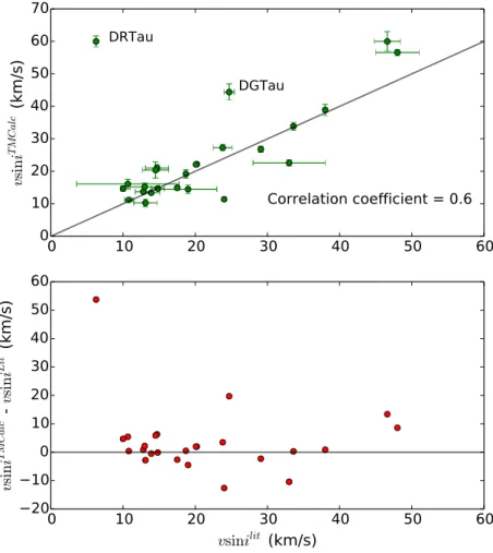
2.1.3 Veiling and projected rotational velocity . . . 30

2.2 Outflow activity parameters . . . 35

2.2.1 Projected terminal velocities . . . 36

2.2.2 Mass loss rates . . . 38

2.3 Conclusions . . . 43

3 Accretion activity among low-mass YSOs in the Orion Nebula Cluster 45 3.1 Introducing the Orion Nebula Cluster . . . 46

3.2 Observations and data reduction . . . 47

3.3 Results . . . 49

3.3.1 Extinction and spectral type . . . 49

3.3.2 Stellar luminosity, radius, mass and age . . . 52

3.3.3 Accretion analysis . . . 53

3.4 Discussion . . . 62 3.4.1 JW180 . . . 64 3.4.2 JW293 and JW908 . . . 64 3.4.3 JW647 . . . 64 3.4.4 JW847 . . . 65 3.5 Conclusions . . . 66

4 Spectroscopic and photometric variability in CTTSs 67 4.1 Data for RY Tau and SU Aur . . . 68

4.2 Results . . . 69

4.2.1 Photometric variability . . . 69

4.2.2 Spectroscopic variability . . . 76

4.2.3 Periodogram analysis . . . 80

4.3 Conclusions . . . 87

5 Simulating the circumstellar environment of CTTSs 89 5.1 Ideal MHD equations for astrophysical plasmas . . . 90

5.2 An outflow model as a starting point . . . 91

5.3 The analytical solution and the initial setup . . . 94

5.4 Before and after implementing of a dead zone . . . 96

5.5 PLUTO setup . . . 98 5.6 Conversion factors . . . 99 5.7 Results . . . 100 5.7.1 Preliminary tests . . . 100 5.7.2 Selected tests . . . 105 5.7.2.1 Mass fluxes . . . 114

5.7.2.2 Outflow and accretion velocities . . . 116

5.7.2.3 Re-scaling the simulations . . . 117

5.8 Discussion . . . 118

5.8.1 Preliminary tests . . . 118

5.8.2 Selected tests . . . 120

5.9 Conclusions . . . 121

6 Conclusions 123 6.1 What has been done . . . 123

6.2 Limitations and perspectives . . . 125

A Best χ2 minimization fits 141

B Observational log and complementary figures for RY Tau and SU Aur 147

1.1 Stages in star formation . . . 2

1.2 Hertzprung-Russel diagram for TTSs in the Taurus-Auriga molecular cloud 3 1.3 Comparison between CTTS and WTTS spectra . . . 4

1.4 Illustration of magnetospheric accretion in a Classical T Tauri star . . . 4

1.5 Illustration of P Cygni and inverse P Cygni profiles . . . 5

1.6 Evolution of spectral energy distributions for low-mass YSOs . . . 6

1.7 Protoplanetary disk of TW Hya imaged with ALMA . . . 7

1.8 Protoplanetary disk images from ALMA . . . 7

1.9 H-band image of IM Lup from SPHERE . . . 8

1.10 Star-disk magnetic interaction . . . 10

1.11 Accretion rate versus stellar mass for low-mass YSOs . . . 10

1.12 Evolution of the angular velocity of a solar mass star according to Gallet & Bouvier (2013) models . . . 11

1.13 Outflow mechanisms in low-mass stars . . . 12

1.14 Conical winds in a slow rotating magnetized star . . . 14

1.15 Compression of the magnetosphere by the disk radial velocity . . . 14

1.16 Illustration of the differential rotation between the star and its circumstellar disk . . . 14

1.17 Images of the HH 34 jet taken by the NASA/ESA Hubble Space Telescope . 15 1.18 RY Tau disk and jet captured by ALMA in the millimeter . . . 16

1.19 Evolution of magnetospheric ejections . . . 16

2.1 Distribution of the spectral types in the sample . . . 21

2.2 Flowchart illustrating the determination of stellar parameters in YSOs with ARES and TMCalc . . . 22

2.3 Illustration of the equivalent width of an absorption line. . . 22

2.4 Illustration of the conservation of the equivalent width with stellar rotation 23 2.5 Comparison between the effective temperatures computed and the literature 26 2.6 Adding artificial veiling to a main-sequence star, HD4208 . . . 28

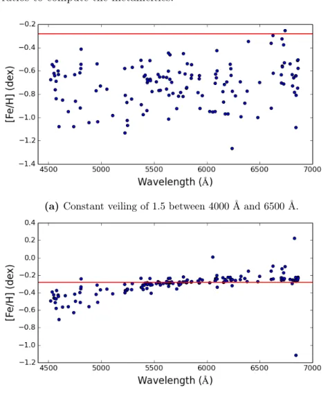
2.7 Individual metallicity estimations in function of the wavelength . . . 30

2.8 Comparison between the projected rotational velocities computed and the literature . . . 33

2.10 Decomposition of forbidden oxygen emission line into a LVC and a HVC . . 37

2.11 Velocity profiles for the forbidden line of oxygen . . . 39

2.12 Comparison between the mass loss rates estimated in this work and the ones from Hartigan et al. (1995) . . . 42

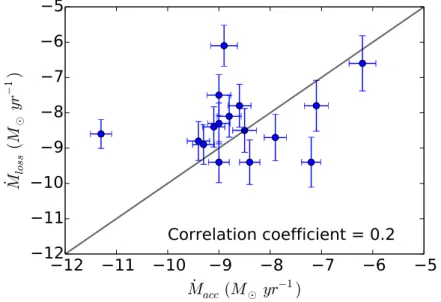
2.13 Accretion rates versus mass loss rates in the sample of CTTSs . . . 43

3.1 Wide-field image of Orion constellation . . . 46

3.2 Position of the targets in the ONC . . . 47

3.3 Target spectrum after extinction correction and the corresponding template 50 3.4 Hertzsprung-Russel diagrams using Siess et al. (2000) and Baraffe et al. (2015) evolutionary tracks and isochrones . . . 54

3.5 Ultraviolet spectra for the ONC targets . . . 56

3.6 Balmer emission lines in velocity scale for JW647 . . . 57

3.7 He I emission profiles at 667.8 and 1082.9 nm for JW647 in velocity scale . 57 3.8 Ca II K and H emission profiles at 393.4 and 396.8nm, respectively, for JW847 59 3.9 Spectral energy distributions for the ONC targets. . . 61

3.10 SEDs of a full-disk, pre-transitional disk and transitional disk an correspond-ing illustration . . . 63

4.1 Light curves for RY Tau and SU Aur . . . 70

4.2 Diagrams with Hα profile in velocity and its correlation with V-magnitude for RY Tau and SU Aur . . . 72

4.3 Diagrams with Hα profile in velocity and its correlation with V-magnitude for each observational epoch of RY Tau . . . 73

4.4 Diagrams with Hα profile in velocity and its correlation with V-magnitude for each observational epoch of SU Aur . . . 75

4.5 The eggbeater model proposed by Johns & Basri (1995b) for SU Aur . . . . 77

4.6 Velocity profiles for the Hα emission in RY Tau . . . 77

4.7 Velocity profiles for the Hα emission in SU Aur . . . 78

4.8 Widths measured for the Hα emission profile . . . 78

4.9 Comparison between the stellar brightness and several parameters related with the Hα emission line for RY Tau and SU Aur . . . 81

4.10 Hα periodograms for RY Tau . . . 85

4.11 Hα periodograms for SU Aur . . . 86

5.1 Illustration of the implementation of accretion . . . 96

5.2 Illustration of the implementation a dead zone and an accretion column . . 97

5.3 Density plots for some preliminary tests with dead zones . . . 103

5.4 Density plots for the selected simulations . . . 106

5.5 Mass flux plots for the selected simulations . . . 109

5.6 Density plots for Test D+ showing the release of magnetospheric ejections . 112 5.7 Mass flux plots for Test D+ . . . 113

5.8 Evolution of mass loss and accretion rates for the selected PLUTO simulations 115 5.9 Illustration of the regions where the mass fluxes were measured. . . 115

5.10 Illustration of the terminal velocity of the stellar jet . . . 116 5.11 Evolution of the maximal accretion velocity and terminal velocity of the jet

for the selected PLUTO simulations . . . 117 A.1 Best fits between synthetic and target spectra of CTTSs . . . 141 B.1 Hα periodograms for RY Tau for each observational epoch . . . 154 B.2 Hα periodograms for RY Tau for each observational epoch for a FAP of 0.5%156 B.3 Hα periodograms for SU Aur for each observational epoch . . . 158 B.4 Hα periodograms for SU Aur for each observational epoch for a FAP of 0.5% 159

2.1 Stellar parameters available in the literature . . . 20

2.2 Stellar parameters derived with ARES and TMCalc . . . 25

2.3 Stellar parameters derived with TMCalc for HD4208 . . . 29

2.4 Veiling and projected rotational velocity computed for HD4208 . . . 32

2.5 Comparison between the veiling determined in this study and the one in the literature . . . 35

2.6 Outflow parameters derived for the targets . . . 41

3.1 Stellar parameters available in the literature for the ONC targets . . . 48

3.2 Observation log of VLT/X-shooter spectra . . . 48

3.3 Observation log of VLT/X-shooter standard tellurics . . . 49

3.4 Spectral indices used to determine the spectral type of the targets . . . 51

3.5 Stellar parameters derived for the ONC targets . . . 51

3.6 List of templates selected for this work. . . 52

3.7 Coefficients needed to determine the mass accretion rates . . . 59

3.8 Logarithmic mass accretion rates derived for the ONC targets . . . 60

4.1 Details on the telescopes/instruments for the spectroscopic observations . . 68

4.2 Variability of the V-magnitudes for RY Tau . . . 69

4.3 Variability of the V-magnitudes for SU Aur . . . 69

4.4 Correlation coefficients between stellar V-magnitude and other parameters obtained from the Hα emission line for RY Tau . . . 80

4.5 Correlation coefficients between stellar V-magnitude and other parameters obtained from the Hα emission line for SU Aur . . . 80

5.1 Configuration of the simulations. . . 105

5.2 Re-scaling the simulations to other CTTSs . . . 119

B.1 Observational log for RY Tau spectra . . . 147

B.2 Observational log for SU Aur spectra . . . 151

2MASS 2Micron All-Sky Survey

AAVSO American Association of Variable Star Ob-servers

AU Astronomical Unit CMEs Coronal Mass Ejections CTTSs Classical T Tauri stars EW Equivalent Width FAP False Alarm Probability HH Herbig-Haro

HR Hertzprung-Russel

HVC High-Velocity Component IPC Inverse P Cygni

IRAF Image Reduction and Analysis Facility LVC Low-Velocity Component

MEs Magnetospheric Ejections MHD Magnetohydrodynamics MIR Mid-Infrared

MRI Magnetorotational Instability MS Main Sequence

Myr Million years NIR Near-Infrared

ONC Orion Nebula Cluster PMS Pre-Main Sequence

SED Spectral Energy Distribution SNR Signal-to-Noise Ratio

TTSs T Tauri stars

UES Utrecht Echelle Spectrograph UVB Ultraviolet

VIS Visible

WTTSs Weak line T Tauri stars YSOs Young Stellar Objects

1

Introduction

Les gens ont des étoiles qui ne sont pas les mêmes. Pour les uns, qui voyagent, les étoiles sont des guides. Pour d’autres elles ne sont rien que de petites lumières. Pour d’autres, qui sont savants, elles sont des problèmes.

—Antoine de Saint-Exupéry, Le Petit Prince

One of the astonishing facts we learn during our childhood is that the Sun is the closest star to planet Earth. As we grow up, we start asking ourselves how did it form? What were the physical processes involved in the formation of the Sun? What impact the evolution of the Sun had on the formation of the planets as we know nowadays? Is there any other way we can look backwards in time to better understand all the mechanisms involved? Are there any other stars similar to the Sun? All the answers are hidden in low-mass Pre-Main Sequence (PMS) stars called T Tauri stars (TTSs). These Young Stellar Objects (YSOs) can be seen as teenage Suns that are still forming and contracting towards the Main Sequence (MS). By observing and studying them, we are getting a step closer towards the understanding of the formation of our own Solar System.

In this chapter, we briefly describe the formation and evolution of low-mass stars. In addition, we characterize these objects through their spectral features and explore accretion an outflow processes enrolled in their evolution. Finally, we mention the goals of the present thesis and describe how is it structured.

1.1

State of the art

1.1.1 Formation of low-mass stars

In our Galaxy, we can find massive structures that gather all the fundamental conditions to generate stars. They are named molecular clouds, are rich in gas and interstellar dust grains and host dense cores, as illustrated in Fig.1.1a. In these denser regions inside cold molecular clouds, protostars are born from gravitational collapse (Stahler & Palla 2005). At this stage, the protostar is embedded in an opaque cloud and can only be seen in the infra-red (Fig.1.1b and c). When the star becomes visible in optical wavelengths (Fig.1.1d), it is possible to determine its position in the Hertzprung-Russel (HR) diagram. Before reaching the main sequence, the PMS star is fully convective, has approximately the same effective temperature, but starts to decrease its luminosity along the Hayashi track (Hayashi 1961). Later on, the star begins to develop a radiative core, the effective temperature increases, but the stellar luminosity is approximately the same along the Henyey track (Henyey et al. 1955). As the PMS stars begin to developed a radiative core and the convective envelope gets thinner, their magnetic fields will become more complex.

Before reaching the main-sequence, PMS stars have temperatures that are not high enough to start burning hydrogen into helium. In order to start these nuclear reactions in their central region, stars need to reach a temperature of ∼ 107K. Until there, their central temperature will increase gradually due to their on-going contraction processes towards the main sequence. By the time the star reaches the MS, it has developed a radiative core surrounded by a convective envelope. These fully formed stars are in hydrostatic and thermal equilibrium. What is supporting the gravitational collapse of these objects is their internal thermal pressure (Petrov 2003; Stahler & Palla 2005).

1.1.2 A closer look on T Tauri stars

T Tauri stars were named after the prototype T Tauri was found by the astronomer John Russel Hind (Hind 1856; Cox 2008). This group of low-mass stars were first studied by Joy (1945) and Herbig (1962), and have been characterized as variable Sun-like stars. TTSs have stellar masses that can go up to 2-3 M and ages ranging between 1 and 10 Million

years (Myr). In the HR diagram, these objects are located at the right side of the main sequence, as shown in Fig.1.2 for TTSs observed in the Taurus-Auriga star-forming region (Stahler 1988).

Figure 1.2: Hertzprung-Russel diagram for TTSs in the Taurus-Auriga molecular cloud. The solid lines correspond to the evolutionary tracks from Iben (1965) and Grossman & Graboske (1971), for pre-main sequence stars, along with the corresponding stellar masses in M. The heavy solid line represents the birthline of Stahler (1983). From Stahler (1988).

TTSs mark a particular evolutionary phase in low-mass stars. Their emission spec-tra resemble the one from the solar chromosphere (Joy 1945). Their specspec-tral types vary between F and M. This evolutionary stage corresponds to the time at which these PMS stars become optically visible and they can be classified in two types. Classical T Tauri stars (CTTSs) are known for having strong ultraviolet and optical emission lines, namely Balmer lines, neutral and ionized metals. In addition, their spectra can also show traces of chromospheric activity. One particular emission is the Hα line, characteristic in YSOs and which can be easily identified in Fig.1.3 at 6563 Å. CTTSs also show the lithium line in absorption at 6708 Å, which is characteristic of young stellar objects. In addition, they are surrounded by accretion disks, which are responsible for the infrared excess fingerprinted in their spectra. Conversely to CTTSs, Weak line T Tauri stars (WTTSs) lack strong emis-sion lines, as shown in Fig.1.3 for V830 Tau spectrum. This evolutionary stage is usually

observed in YSOs with ages higher than 10 Myr, when their disks start to dissipate.

Figure 1.3: Comparison between CTTS (DR Tau and BP Tau) and WTTS spectra (V830 Tau). From Stahler & Palla (2005).

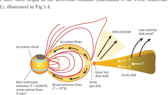
In the spectra of CTTSs, the emission lines originate from different regions of the star-disk system with different densities and temperatures. Most of the permitted emission lines have their origin in the accretion columns (Hartmann et al. 1994; Muzerolle et al. 2001), illustrated in Fig.1.4.

Figure 1.4: Illustration of magnetospheric accretion in a Classical T Tauri star. From Hartmann et al. (2016).

On one hand, strong emissions, as Hα, with broad profiles are thought to have their origin in an extended region in the magnetosphere (Calvet et al. 1984; Takami et al. 2003). Depending on the line of sight, the observer may also detect in the Balmer lines blueshifted and/or redshifted absorptions, which are typical outflow and inflow signatures, respectively. One of the most discussed emissions is probably Hα, not only emitted on the stellar surface and at the base of the accretion columns (Dodin 2015), but also in the wind and magnetospheric region (Kurosawa et al. 2011). If there is enhancement of

outflow/accretion activity, the corresponding absorptions will get stronger and go below the continuum. In that case, we are in the presence of a P Cygni profile, for the blueshifted absorption, or a Inverse P Cygni (IPC) in case of a redshifted absorption (e.g Edwards et al. 1994; Reipurth et al. 1996). In Fig.1.5 both profiles are shown.

Figure 1.5: Illustration of P Cygni (left) and inverse P Cygni (right) profiles. From Reipurth et al. (1996).

On the other hand, narrow emission lines such as He I, should be created near the accretion shock region (Hartmann et al. 2016). Besides accretion tracers, the spectra of CTTSs can also show blueshifted emission of low-excitation lines formed in outflows, namely forbidden lines such as [OI] (Herbig 1962). Forbidden lines originate from rarefied gas flows and form at large distances from the YSO higher than 1 Astronomical Unit (AU) and have two components, a High-Velocity Component (HVC) and a Low-Velocity Component (LVC). While the HVC has been associated with the presence of a stellar jet, the LVC is probably linked with slower outflows, namely disk winds.

Besides showing a very rich emission line spectrum, CTTSs have also been characterized by irregular light variability and variable accretion and outflow activity detected through emission line profiles. The time scale variability can be daily, or even take place in only few hours (e.g. Chou et al. 2013; Petrov et al. 2019). According to Herbst et al. (1994), irregular variability in TTS can be explained by three reasons. First, the presence of cold spots due to magnetic activity that is mainly observed in WTTSs. Second, accretion of circumstellar material and, consequently, the presence of hot spots on the stellar surface due to on-going accretion in CTTSs. Hot spots have a shorter life-time compared to cold spots. Third, obscuration of the central star by circumstellar dust that leads to an increase of visual extinction in the line of sight seen in both CTTSs and WTTSs.

The presence of circumstellar disks is due to the angular momentum conservation all along the collapse of the protostellar core, which lead to the settling of gas and dust in a disk (Shu 1977). Disks can be detected through the presence of infrared excess emission in the spectra of TTSs. Depending on the distance to the star, circumstellar material will have different temperatures. Warmer material will have higher temperatures if it is closer to the YSO, while cooler material will be further away in the disk (Williams & Cieza 2011).

This IR excess can be quantified through the infrared spectral index given by

αIR=

d log νFν

d log ν , (1.1)

where ν corresponds to the frequency and νFν is the flux density. Different ranges of the

αIR index will correspond to a different class, according to the works of Lada & Wilking

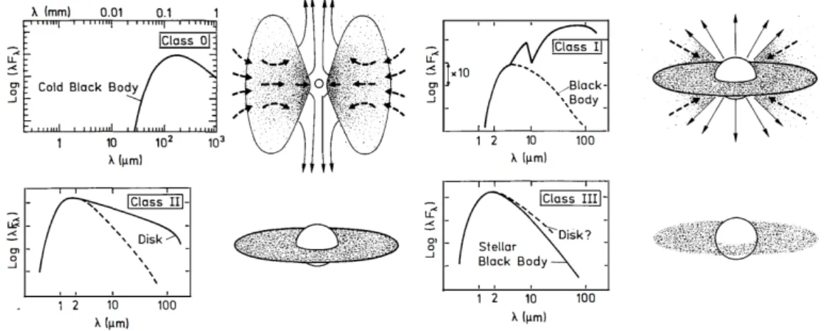
to the slope of the Spectral Energy Distribution (SED), measured between 2 and 25µm, the classes are defined as

• Class 0: YSO is deeply buried in the cloud and there is no optical or near-infrared emission. They can only be detected at far-infrared and millimeter wavelengths (Andre et al. 1993).

• Class I: αIR > 0.3, YSO is still inside a dense core in the cloud and is optically

obscured.

• Flat spectrum: −0.3 < α_IR < 0.3, intermediate stage between class I and II intro-duced by Greene et al. (1994).

• Class II: −1.6 < α_IR< −0.3, less embedded stars surrounded by a circumstellar disk and corresponding to the CTTS evolutionary stage.

• Class III: α_IR < −1.6, the disk begins to disperse and accretion activity is ceasing. This stage is compatible with WTTSs.

Figure 1.6: Evolution of spectral energy distributions for low-mass YSOs. Adapted from André (1994).

As the interstellar medium is composed by 99% of gas and 1% of dust, so are the disks in their initial stage (e.g. Williams & Cieza 2011; Ercolano & Pascucci 2017). Measuring the size of a disk is a difficult task, since the emission of the distant and cooler circumstellar material is hard to detect. Estimates indicate that disk sizes range between 20 and 200 AU (Williams & Cieza 2011). These structures have a lifetime typically around 3-5 Myr, but may vary from less than 1 Myr to 10 Myr (Hernández et al. 2008; Williams & Cieza 2011; Gallet & Bouvier 2013; Gorti et al. 2016; Ercolano & Pascucci 2017).

According to Lissauer et al. (2009), disks seem to live enough so that planets can form. Besides planet formation, other main processes involved in disk dispersal are accretion and disk winds. On one hand, accretion enables the transport of material from the disk to the star and angular momentum in the opposite direction. On the other hand, photoevapora-tion enables the formaphotoevapora-tion of thermal winds that result from the escape of gas in the disk atmosphere that is heated by the star (e.g. Gorti et al. 2016; Ercolano & Pascucci 2017).

Disks are the potential birthplaces of future planets and infrared interferometry has been an important tool to provide information about the inner regions of star-disk systems in YSOs (Millan-Gabet et al. 1999; Akeson et al. 2000). The development of high-advanced instruments and imaging techniques has provided staggering images of YSOs surrounded by their disks.

Since the first promising results of (sub-)millimeter ALMA observations for the well-know YSO HL Tau (ALMA Partnership et al. 2015), there has been a paper-boom with images of protoplanetary disks as never seen before. Some examples include the face-on disk of TW Hya in Fig.1.7 (Andrews et al. 2016) and other YSOs with different disk morphologies in Fig.1.8 (Andrews et al. 2018). Other interesting protoplanetary disks can be seen in the works from van der Marel et al. (2015); Ansdell et al. (2016); Barenfeld et al. (2016); Pascucci et al. (2016); Cieza et al. (2017); Fedele et al. (2017); van der Plas et al. (2017); Boehler et al. (2018); Cazzoletti et al. (2018); Long et al. (2018) and van der Marel et al. (2019). At the time this thesis was written, more than 100 protoplanetary disks were captured with high-resolution imaging from ALMA.

Figure 1.7: Protoplanetary disk of TW Hya imaged with ALMA. The beam sizes are shown as well as a bar scale corresponding to 1 and 10 AU. From Andrews et al. (2016).

Figure 1.8: Protoplanetary disk images from ALMA. The beam sizes are shown as well as a bar scale corresponding to 10 AU. From Andrews et al. (2018).

There is an additional, and promising, new instrument that is giving a big contribution for the study of circumstellar disks in YSOs, which is SPHERE, installed at the Very Large Telescope. There are remarkable images captured by this instrument in the works of Garufi et al. (2017a) and Avenhaus et al. (2018) (see Fig.1.9). In particular, Müller et al. (2018)

were able to image with this instrument a very young planet orbiting the star PDS 70, also known as V1032 Cen. This planet was found inside a gap of this TTS with an age of approximately 5 Myr. More recently, Haffert et al. (2019) discovered a second planet orbiting the same star. They concluded that both protoplanets are still accreting material from the disk. According to Williams & Cieza (2011), exoplanets have been found in 10% of the Sun-like stars in the vicinity of the Solar System.

Figure 1.9: H-band image of IM Lup from SPHERE. The scale bar corresponds to 100 AU. The red dot corresponds to the position of the star, while green areas correspond either to bad pixels or regions hidden by the coronagraph. From Avenhaus et al. (2018).

The high amount of high-resolution images of disks in YSOs, revealed that there is a large morphological variety of protoplanetary disks. In view of this, Garufi et al. (2017b) have been working on the taxonomy of these objects based on their infrared spectral energy.

1.1.3 Accretion

Shakura & Sunyaev (1973) and Lynden-Bell & Pringle (1974) proposed models to explain the concept of accretion disk that can be applied in different astrophysical objects. In agreement with Kepler’s laws, the material in the disk rotates differentially. This assump-tion is only valid if the central star mass is much larger than the disk. Due to the presence of viscosity, the circumstellar material will have its rotation energy converted into thermal energy, implying emission from the disk (Petrov 2003). In Shakura & Sunyaev (1973), the material viscosity is represented by the parameter α, which corresponds to the ratio of stress over pressure.

Years later, the rediscovery of the Magnetorotational Instability (MRI), by Balbus & Hawley (1991), provided a plausible explanation for the α parameter in Shakura & Sunyaev (1973) accretion model. MRI is the product of the interaction between a weak magnetic field and a disk that is differentially rotating (i.e. the angular velocity decreases outward). Very briefly, disk turbulence, which is generated by fluid instabilities, is needed to induce accretion. MRI generates and allows the redistribution of angular momentum to enable

accretion through the disk (Balbus 2003).

Bertout et al. (1988) applied for the first time the accretion disk theory to TTSs by using a model with an active PMS star and an accretion disk similar to the one in Lynden-Bell & Pringle (1974). According to the authors, between the star and the disk there is a boundary layer, i.e. a shock front, at the equatorial plane. The emerging radiation from this region could explain the excess emission observed at ultraviolet wavelengths.

The magnetospheric accretion model has been generally accepted by the scientific com-munity in order to characterize the way accretion is processed in a low-mass pre-main sequence star. Originally conceived for neutron stars by Ghosh & Lamb (1979), it was later adapted for CTTSs by Uchida & Shibata (1984), Camenzind (1990) and Koenigl (1991). This model suggests that the circumstellar disk is truncated in its inner region close to the star, thanks to the presence of strong magnetic fields, around 1-3 kG (e.g. Johns-Krull 2007)1. In this inner edge of the disk, the stellar magnetosphere is strong enough to funnel the disk material onto the stellar surface through accretion columns. In these funnel flows, the gas can reach temperatures around 8000 K. It is thought that in these same columns the Hα line is emitted. The corresponding emission will translate into broadened velocity profiles (Muzerolle et al. 1998b, 2000). When the material falls onto the surface of the star, near the star’s magnetic poles, with a velocity between 200 and 300 km s−1, it creates a shock region. The shock region can reach temperatures near 106 K, but the average temperature of spot is about 104 K (Kenyon et al. 1994; Hartmann et al. 2016).

Romanova et al. (2004) discovered through 3D simulations that hot spots have an inhomogeneous structure and their shape depends on the magnetic axis inclination. The smaller the tilt, the bigger the shape. Higher tilts imply spots with bar shapes. In Kulkarni & Romanova (2013), simulations were made to study the shape and structure of these shock regions. They found out that the density and temperature of a hot spot increases towards its interior. This implies that the central region of the spot will be responsible for emission in the X-rays waveband, while the surrounding regions will emit in the ultraviolet, optical and infrared. In this region, temperatures can increase up to 106 K and the release of ultraviolet energy will be responsible for adding a continuum excess emission in the spectra of CTTSs (Valenti et al. 1993; Calvet & Gullbring 1998). This emission will make the photospheric absorption lines appear less deep when compared to non-accreting YSOs of the same spectral type. This effect is known as veiling, which tends to be stronger towards shorter wavelengths (Hartmann et al. 2016).

In order to enable the formation of accretion columns in the star-disk system, magnetic braking is needed (Bouvier et al. 2007). This is only possible if the truncation radius, R_t, is less than the co-rotation radius, Rco, as illustrated in Fig.1.10.

On average, accretion processes in CTTSs can last for 2 to 3 Myr. A typical value for the average accretion rate in these low-mass YSOs has been estimated to be around 10−8 Myr−1 (Hartmann et al. 2016), as shown in Fig.1.11. Typical ratios between the

jet mass loss and accretion rates range between 1% and 10% (Hartigan et al. 1995; White

1

For comparison, the average intensity of the solar magnetic field is less than 4 G and the one from planet Earth ranges between 0.25 and 0.65 G (e.g. Bouvier et al. 2007; Finlay et al. 2010).

Figure 1.10: Star-disk magnetic interaction. The existence of accretion columns is possible as long as the truncation radius, Rt, is smaller than the co-rotation radius, Rco. From Matt & Pudritz (2004).

& Hillenbrand 2004; Cabrit 2007).

Figure 1.11: Accretion rate versus stellar mass for low-mass YSOs. Different symbols correspond to accretion rates measured in the literature through different methods, namely from the Balmer continuum (red circles), photometric U-band measurements (blue diamonds), and emission lines (green squares). From Hartmann et al. (2016).

The magnetic field plays a key role not only in the star-disk interaction, but also in regulating angular momentum extraction. Although Fig.1.4 shows a simplistic view of the topology of a dipolar magnetic field, recent studies involving Zeeman-Doppler imaging show that the topology of magnetic fields in low-mass YSOs is more complex. One example is given in Donati et al. (2007), where the magnetic field geometry of V2129 Oph, a CTTS, is dominated by a 1.2 kG octupole, tilted by about 20◦ with respect to the rotation axis. Another case is given by Long et al. (2011), where BP Tau has a 1.2 kG dipole and an octupole field of 1.6 kG, which is stronger at the surface of the star comparatively to the dipole.

Stellar rotation has an impact not only in the internal structure of the star, but also on their magnetic activity (Bouvier et al. 2014). If YSOs conserved their angular momentum,

we would expect that accretion would contribute to the spin-up of the star rotation velocity, while the star is still contracting towards the main sequence. This is shown in Fig.1.12, where the dotted lines correspond to the expected evolution of the rotation rate in a 1 M star (Bouvier et al. 2014). However, observations contradicted this idea. The rotation

period measured for CTTSs is not the same for WTTSs. CTTSs rotate slower (3 to 10 days) compared to WTTSs (1 to 7 days) (Bouvier et al. 2014). Models from Gallet & Bouvier (2013) are in agreement with the observed values for the angular velocities measured for solar-type stars in young open clusters. These models include a constant angular velocity during the disk accretion epoch in the early PMS and are based on numerical simulations of magnetized stellar winds by Matt et al. (2012), from which Gallet & Bouvier (2013) quantify the angular momentum losses.

In Fig.1.12, we can see that the red and blue lines, which correspond to the evolution of the rotation velocity according with Gallet & Bouvier (2013) models, show different profiles compared to the dotted ones due to the loss of angular momentum. As long as the star is interacting with the disk, the angular speed is going to fall below the predicted one. Once the disk starts to dissipate, the angular speed increases and overlaps with the theoretical profile.

Figure 1.12: Evolution of the angular velocity of a solar mass star according to Gallet & Bouvier (2013) models (red and blue lines). The evolution of the rotation rate if the star conserved its angular momentum is also shown (dotted lines). From Bouvier et al. (2014).

Previously, we mentioned that is possible to detect accretion through emission lines in CTTSs spectra. But how can we quantify accretion? One way is through the use of ac-cretion luminosities. These are derived from acac-cretion continuum measurements in which a bolometric correction is applied (Hartmann et al. 2016). Accretion luminosities can be derived either from the excess Balmer continuum emission or from the Balmer jump in ultraviolet wavelengths (e.g. Bertout et al. 1988; Valenti et al. 1993), from veiling mea-surements (e.g. Hartigan et al. 1995), or even from U-band photometry (e.g. Manara et al. 2013). Mass accretion rates can also be estimated from emission lines. This method relies on measuring the line flux, convert it to line luminosity, then to accretion luminosity and finally to mass accretion rate, based on accretion luminosity and line luminosity empirical relations derived for several stars (e.g. Rigliaco et al. 2012; Alcalá et al. 2014, 2017).

1.1.4 Outflows

It has been debated that the disk-locking paradigm could give a plausible explanation for the spin-down of YSOs, as proposed for neutron stars in Ghosh & Lamb (1979). If the disk and the star are trapped by the magnetic field, this should be responsible for slowing down the rotation of the star. The stellar rotation is higher than the rotation of the disk. If a strong magnetic field connects the star to the disk, this will imply the deceleration of the star.

Nevertheless, there are new studies that suggest that there should be other angular momentum removal mechanisms responsible for slowing down these objects efficiently, namely outflow mechanisms (see Fig.1.13). As mentioned previously, outflows can be detected through forbidden emission lines or blueshifted absorptions present in the profiles of permitted emission lines (Bouvier et al. 2007). Those outflows can be shaped as stellar winds (Matt & Pudritz 2005), disk winds (Blandford & Payne 1982), X-winds (Shu et al. 1994), conical winds (Romanova et al. 2009), or even Magnetospheric Ejections (MEs) (Goodson et al. 1997; Zanni & Ferreira 2013). According to Ferreira (2013), the Ghosh & Lamb (1979) model, X-winds, conical winds and the accretion powered stellar winds cannot spin-down the star, contrary to magnetospheric ejections. Indeed, it seems very difficult that only one mechanism is responsible for the angular momentum removal observed in CTTSs. Most likely, the spin-down is processed by a combination of different outflows jointly with the contribution of magnetospheric accretion processes.

Figure 1.13: Outflow mechanisms in low-mass stars. From Romanova & Owocki (2015).

1.1.4.1 Stellar winds

Stellar winds could give an explanation for slowing down the stellar rotation. We know that for the Sun, the angular momentum removal is due to stellar winds (e.g. Parker 1958). One of the promising works is given by the accretion-powered stellar winds models by Matt & Pudritz (2005). These outflows would be sustained by a fraction of energy released by accretion processes. According to the authors, if the mass loss rate in the stellar winds is around 10% of the accretion rate, it should be enough to break the spin-up of the star. Assuming that stellar winds are powered by accretion, Matt & Pudritz (2008) suggest that the mass loss rate of the wind should be equal to or less than 60% of the accretion rate. Above this value accretion is not possible to power the wind.

The modelling performed in Sauty et al. (2011) shows that jets can efficiently brake a CTTS. One of the presented solutions suggests that close to the star, with a dipolar

magnetic field configuration, the wind is more efficient concerning the extraction of angular momentum.

1.1.4.2 Disk winds

Extended disk winds are magneto-centrifugally accelerated from the corresponding Ke-plerian disk (e.g. Blandford & Payne 1982). This kind of outflows may be sufficient to spin-down the disk, but is not enough to decelerate the star (Cabrit 2007; Ferreira 2013).

1.1.4.3 X-winds

X-winds are a product of the interaction between the star’s magnetosphere and the cir-cumstellar disk. The X-region separates two regions at a co-rotation radius RX. The

disk material close to the inner region of R_X rotates at sub-Keplerian velocities favouring accretion. The disk material close to the exterior region of RX rotates at super-Keplerian

velocities enabling the escape of the disk material through a wind. At RX the stellar

an-gular velocity equals the Keplerian velocity of the disk (Ω = q

GM∗/R3_X). In this process

there is angular momentum that is transported from the accretion flow to the interior re-gion of RX. In addition, and outside RX, the X-wind transports angular momentum from

that region towards the interstellar medium. The angular momentum transfer from the accretion column to the outflow regulates the spin-up of the star.

1.1.4.4 Conical winds

Romanova et al. (2009) have simulated a different shape of winds for slowly rotating stars named conical winds, which are driven by magnetic pressure (see Fig.1.14). The outflows are conically-shaped, have a half-opening angle between 30 and 40◦ and are composed by 10 to 30% of the inner disk material, up to 0.3 AU from the star. Besides the conical winds, Romanova et al. (2009) managed to simulate also a jet inside the conical wind region. The launching mechanism of these outflows results from compression of the magnetosphere by the radial velocity of the material in the circumstellar disk, as shown in Fig.1.15. There are some differences between the X-wind and the conical wind models. First, the X-wind model requires that the truncation radius coincides with the co-rotation radius, while in conical winds the truncation radius can be smaller than the co-rotation radius. This means that, in the second model, the star can rotate more slowly than the inner disk. Second, the X-winds are driven by the centrifugal force, while the conical winds are magnetically pressure driven (Romanova & Owocki 2015). Due to the star-disk differential rotation, the magnetic field lines will inflate as illustrated in Fig.1.16 . In the work of Romanova et al. (2009), this leads to the release of winds, from the inner disk region, with a conical shape.

1.1.4.5 Jets

The origin and structure of jets has been under debate since many decades. Ferreira et al. (2006) mention that outflow processes in CTTSs should result from a mixture of different processes, namely a disk wind, a coronal stellar wind and hot material ejected

Figure 1.14: Conical winds in a slow rotating magnetized star. The background corresponds to the mass flux, the arrows to the poloidal velocity and the solid yellow lines represent the magnetic field lines. From Romanova et al. (2009).

Figure 1.15: Compression of the magnetosphere by the disk radial velocity. From Romanova & Owocki (2015).

Figure 1.16: Illustration of the differential rotation between the star and its circumstellar disk. As the star and the disk rotate at different speeds, the magnetic field lines increase the total magnetic field. The enhancement of magnetic energy density leads to the inflation of the magnetic loops. From Goodson et al. (1997).

from the magnetosphere. Some steady-state models have been developed in order to explain the jets of YSOs. Although the models can be established by the same set of MHD equations, they differ on their corresponding boundary conditions (Ferreira 2013). Models can be based either in stellar winds (Sauty & Tsinganos 1994; Matt & Pudritz 2005), X-winds (Shu et al. 1994) or even disk X-winds (Blandford & Payne 1982). Jets are bipolar and collimated gas flows with opening angles of only few degrees (Ferreira 2013). These structures are perpendicular to the circumstellar disk and can be detected through low excitation forbidden lines. These emitting regions have an extension that ranges between 100 to 500 AU and the average velocity of a jet is close to 170 km s−1 (Beckwith et al. 1996). According to previous works, there seems to be a correlation between the mass loss rate derived through [OI] and the accretion rate estimated through veiling measurements (Cabrit et al. 1990; Hartigan et al. 1995). This suggests that accretion is feeding jet mechanisms.

In addition, these structures can show bright nodes that move towards the interstellar medium and were first detected through Herbig-Haro (HH) objects. HH objects were first observed by Burnham during the end of the 19th century (Burnham 1890), and studied in detail years later by George Herbig and Guillermo Haro (Reipurth & Heathcote 1997). One known case is the jet HH34 shown in Fig.1.17. The knotty structure suggests that jets result from unsteady ejection events (Ferreira 2013). The shock waves generated by jets in the interstellar medium is due to the partial conversion of the kinetic energy of the outflow into thermal motion. In those regions the gas is ionized and heated up to 105 K (Giannini et al. 2015). The forbidden lines will be emitted from the post-shock cooling regions (Fang et al. 2018). Typical mass loss rates measured for jets in CTTSs vary between 10−7to 10−9 Myr−1 (Frank et al. 2014). Although the origin of jets is still not well understood, it is

believed that the acceleration mechanisms could be a product of the star-disk interaction through accretion (Frank et al. 2014).

Figure 1.17: Images of the HH 34 jet taken by the NASA/ESA Hubble Space Telescope. At the left we show the stellar jet of HH 34 in 1994, 1998 and 2007. At the right we show the corresponding composite image of the brightest segments of the HH 34 jet, where Hα is represented in green and [SII] in red. The jet is flowing from left to right. From Hartigan et al. (2011).

More recently, Garufi et al. (2019) obtained with SPHERE the highest spatial resolution image ever obtained for an atomic jet, down to approximately 4 AU. Fig.1.18 shows the disk and jet of RY Tau traced with different elements. According to the authors, the jet seems to shake back and forth and has an extension of approximately 600 AU, detected

through [Fe II] emission.

Figure 1.18: RY Tau disk and jet captured by ALMA in the millimeter. From Garufi et al. (2019).

1.1.4.6 Magnetospheric ejections

Magnetospheric ejections are a product of successive expansion, disconnection and recon-nection events of the magnetospheric field lines. If the anchor points of the accretion columns have different angular velocities connecting the star and the disk, this will lead to the inflation of the magnetic field lines. During the disconnection events, material is ejected towards the interstellar medium.

Goodson et al. (1997), managed to simulate these outflows during the 90’s and con-firmed that these events could have a cyclic behaviour. Years later, Zanni & Ferreira (2013) simulated several cycles of MEs resulting from the interaction between the dipolar magnetic field and the circumstellar disk. They concluded that the MEs regulate stellar rotation not only by removing angular momentum in the inner region of the disk, but also by extracting it directly from the star due to the differential rotation between the star and the outflowing material. The MEs propagate between the stellar wind and disk wind regions, as shown in Fig.1.19. These outflows are similar to Coronal Mass Ejections (CMEs) that we can see in the Sun (Romanova & Owocki 2015).

Figure 1.19: Evolution of magnetospheric ejections. The background corresponds to logarithmic density, the solid lines represent the magnetic field lines and the blue arrows correspond to veloc-ity. The yellow lines correspond to the evolution of the same magnetic field line throughout the simulation. Time is expressed in stellar rotations. From Zanni & Ferreira (2013).

1.2

Goals and structure of the thesis

The purpose of the current thesis is to show that we can improve our knowledge on Clas-sical T Tauri stars by joining both observational and numerical perspectives. Since a few decades ago, the physical mechanisms involved in the formation and evolution of YSOs can be more easily explored through models and numerical simulations constrained by observational data. In view of this, the aim of this thesis is to explore not only observa-tional data of CTTSs, but also numerical simulations aiming to reproduce what we see. By shaping numerical tests with observational constraints and playing with the main physical quantities, we intend to model accretion and outflow phenomena that could characterize the circumstellar environment of a well known CTTS, RY Tau. This could be fruitful to understand what low-mass YSOs are experiencing in the early stages of their evolution.

The thesis is divided in four parts, followed by the conclusions and three appendices including supplementary information and results through tables and/or plots.

Chapter 2 concerns a sample of CTTSs for which we have tested the determination of stellar parameters with available software. Since in a previous work the mass accretion rates and accretion velocities for these objects were explored, in this work we examine outflow activity parameters. Some of the computed values will be used in Chapter 5 to re-scale numerical simulations aiming to portrait the circumstellar environment of a YSO. Chapter 3 deals with a sample of five low and very-low mass YSOs belonging to the Orion Nebula Cluster. The observations were taken by the X-shooter instrument installed at the VLT. Throughout the chapter is explained how the data reduction was performed and how did we determine their corresponding stellar parameters. We also searched for evidence of accretion activity in the spectra and looked for the presence of circumstellar disks through available on-line photometry.

Chapter 4 is the product of a project developed with P. P. Petrov concerning the analysis of the variability of two CTTSs, RY Tau and SU Aur. Spectroscopic variability is studied through spectral measurements, which are compared with photometric data.

Chapter 5, gathers numerical simulations of the circumstellar environment of CTTSs, based on observational constraints of RY Tau. We give an overview of the outflow model and the analytical solution that rule the simulations, as well as the initial and boundary conditions. Several tests were performed and the most interesting cases are discussed. The numerical results will be compared with the ones we derived for RY Tau in Chapter 4. In addition, we try to extend these results to other objects than RY Tau, but we will see that there are some limitations in doing so.

Finally, Chapter 6 summarizes all the main conclusions from the previous chapters, but also pinpoints which are the limitations found, as well as future perspectives based on the work developed in this thesis.

2

Deriving stellar parameters for

CTTSs

Emission and absorption lines of a spectrum contain information that can be decoded into stellar parameters, which are fundamental to characterize stars. In particular, optical emission profiles can be analysed in order to detect signatures of outflow processes. These are some of the steps taken towards the understanding of the circumstellar dynamics of each YSO.

In this chapter, a sample of 35 CTTSs spectra is analysed. The data were taken by A. Pedrosa in November 1998 and collected with the Utrecht Echelle Spectrograph (UES), installed at the 4.2m William Herschel Telescope, La Palma, before being de-commissioned in 2002. The used slit was 6” long and 1.20” wide, corresponding to a resolution of 51 000. The average signal-to-noise ratio was estimated to be above 40.

Although the spectra were taken more than 20 years ago, the data were never published before. Table 2.1 lists all the targets and corresponding stellar parameters available in the literature and relevant for this work, while Fig.2.1 shows the distribution of the spectral types in the sample. Around 83% of the CTTSs composing the sample are K-type stars, 11% correspond to G-type stars, while only 6% are M-type stars.

From this sample, we determined some typical stellar parameters as effective tempera-ture, projected rotational velocity and veiling. Some outflow parameters were also derived, namely the projected terminal velocity of the jet and mass loss rate, whenever we had in emission a well known outflow tracer, the forbidden line of [OI] at 6300 Å. This emission was corrected with Molecfit (Kausch et al. 2015; Smette et al. 2015) by S. Ulmer-Moll, who removed the telluric absorptions that were contaminating this particular wavelength region (Ulmer-Moll et al. 2019).

(M∗), stellar radius (R∗), inclination (i), projected rotation velocity (v sin i), veiling measured at 5700 Å (r5700) and 6300 Å (r6300). The last column lists all the references from which the parameters were taken.

Object SpT log L∗ M∗ R∗ i v sin i r5700 r6300 References

(L) (M) (R) (◦) (km s−1) AA Ori K4 ... ... ... ... 10.8 ... ... 1,36 AA Tau K7 -0.097 0.76 1.76 75 12.8 0.63 0.0 2,2,15,15,20,37,8,39 AS 353a K5 0.570 0.63 3.30 20 ... 5.10 ... 3,8,8,8,21,8 BM And K5 0.740 1.19 4.03 ... 38.0 ... ... 4,4,15,15,15 BP Tau K7 -0.022 0.75 1.84 36 13.1 0.61 0.6 2,2,15,15,22,37,8,39 BZ Sgr K0 ... ... ... ... ... .. ... 5 CI Tau K7 -0.060 0.76 1.77 46 13.0 0.39 0.6 2,2,15,15,23,37,8,39 CW Tau K3 0.041 1.29 1.96 49 33.0 1.70 1.5 2,2,15,15,24,37,8,39 DF Tau M0 0.301 0.39 3.55 50 46.6 0.66 1.6 1,6,15,15,25,37,8,39 DG Tau K6 0.230 0.90 2.23 32 24.7 3.00 1.0 2,2,15,15,22,37,8,39 DI Cep G8 0.780 1.74 2.31 27 20.2 ... ... 6,6,15,15,26,15 DK Tau K7 0.114 0.74 2.17 44 17.5 0.49 0.4 2,2,15,15,25,15,8,39 DL Ori K1 ... ... ... ... 10.7 ... ... 7,36 DL Tau K7 -0.155 0.57 1.80 40 19.0 1.10 1.0 1,6,15,15,22,37,8,39 DQ Tau K7 -0.020 0.43 2.00 23 14.7 0.18 ... 8,8,8,8,27,37,8 DR Tau K5 0.230 0.74 2.46 69 6.3 9.20 5.6 1,6,15,15,28,37,8,39 DS Tau K5 -0.222 0.99 1.02 65 10 0.96 0.6 1,6,15,15,29,15,8,39 EH Cep K2 ... ... ... ... ... ... ... 1 GK Tau K7 0.146 0.73 2.34 46 18.7 0.23 0.1 2,2,15,15,25,15,8,39 GM Aur K3 -0.155 0.77 1.56 52 14.8 0.22 0.6 1,6,15,15,22,37,8,39 LkHα 191 K0 1.080 2.68 3.97 ... 24.0 ... ... 1,14,15,15,15 LkHα 330 G3 ... 2.50 ... 35 33.6 ... ... 9,16,30,38 RW Aur K2 0.230 1.48 1.71 37 14.5 1.80 ... 10,10,15,15,25,37,8 RY Tau K1 0.881 1.63 2.40 66 48.0 0.10 ... 2,2,8,8,31,37,8 T Tau K0 0.950 2.41 3.44 72 20.1 ... ... 2,2,15,15,32,15 UY Aur K7 0.020 0.75 1.90 42 23.8 0.35 ... 11,11,15,15,33,37,8 UZ Tau E M1.3 0.440 0.18 4.30 56 ... 0.73 ... 1,8,8,8,23,8 V1079 Tau K5 -0.131 1.02 1.54 ... 13.9 ... ... 10,10,15,15,37 V1305 Ori K5 ... ... ... ... 29.1 ... ... 7,36 V1980 Cyg G5-G7 1.420 2.90 5.30 ... ... ... ... 33,14,17,34 V466 Ori K1 ... ... ... ... ... ... ... 12 V625 Ori K6 0.830 1.00 4.67 ... ... ... ... 1,14,15,15 V649 Ori G8 0.910 1.80 4.30 ... ... ... ... 1,14,15,15 V828 Cas K3 ... ... ... ... ... ... ... 35 WY Ari K5 ... 0.80 1.2 35 ... ... ... 13,19,18,19

References: (1) Grankin et al. (2007);(2) Güdel et al. (2007);(3) Rice et al. (2006);(4) Eisner et al. (2007);(5) Torres et al. (2006);(6) Johns-Krull et al. (2000);(7) Fang et al. (2009);(8) Hartigan et al. (1995);(9) Brown et al. (2008);(10) Akeson et al. (2005);(11) Hartmann et al. (1998);(12) Simbad;(13) Luhman (2001);(14) Cohen & Kuhi (1979);(15) Artemenko et al. (2012);(16) Osterloh & Beckwith (1995);(17) Lev-reault (1988);(18) Valenti et al. (1993);(19) Carmona et al. (2007); (20) Cox et al. (2013);(21) Curiel et al. (1997);(22) Guilloteau et al. (2011);(23) Andrews & Williams (2007);(24) Coffey et al. (2008);(25) Appen-zeller & Bertout (2013);(26) Ismailov (2004);(27) Mathieu et al. (1997);(28) Muzerolle et al. (2003);(29) Ake-son & Jensen (2014);(30) Isella et al. (2013);(31) Isella et al. (2010);(32) Ratzka (2008);(33) Close et al. (1998);(34) Rei et al. (2018);(35) Mora et al. (2001);(36) Da Rio et al. (2016);(37) Nguyen et al. (2012);(38) Cottaar et al. (2014);(39) Simon et al. (2016).

G3 G6 G8 K0 K1 K2 K3 K4 K5 K6 K7 M0 M1

Spectral type

0

1

2

3

4

5

6

7

8

9

Number of stars

Figure 2.1: Distribution of the spectral types in the sample.

2.1

Determining stellar parameters with ARES and TMCalc

In this section we developed a method aiming to automatize some procedures used to determine stellar parameters in YSOs. These parameters include effective temperature, projected rotational velocity, veiling and can now be determined automatically through a code in few steps.

Firstly, the effective temperature and metallicity are computed with the software pub-licly available: ARES1 (Automatic Routine for line Equivalent widths in stellar Spectra) (Sousa et al. 2007, 2015) and TMCalc2 (Temperature and Metallicity Calculator ) (Sousa et al. 2012). ARES is a code able to measure automatically the equivalent widths of a given list of weak metal lines. These measurements can be used by TMCalc, which is the software extension for ARES. TMCalc holds a fast code to derive Teff and metallicity for stars of

spectral types F, G and K based on line-ratio calibrations. Both of these programs have been used for main-sequence stars, but have not been applied for pre-main sequence stars since it is needed a high Signal-to-Noise Ratio (SNR) and absorption lines are weaker due to veiling. This study will test somehow the capabilities of the mentioned software when applied to CTTSs. In particular, we will show that is possible to determine the Teff of a

PMS star even if the veiling is high.

Secondly, the projected rotational velocity and veiling are set as free parameters and are determined through a χ2 minimization fit, which will be explained more ahead.

In Fig.2.2 is shown a flowchart illustrating how the script works. Very briefly, the code has as a first input the target spectrum. Then, the spectrum is sent automatically to ARES and TMCalc, where the effective temperature and metallicity are computed. Based on the T_eff determined by the software, a list of templates is selected to compute v sin i and veiling, the two free parameters in the minimization fit. Finally, all the computed param-eters for the target and corresponding templates are printed in a single text file that is given to the user.

In the following subsections, the way each parameter is derived will be briefly explained

1

ARES web page: http://www.astro.up.pt/~sousasag/ares/

2

Figure 2.2: Flowchart illustrating the determination of stellar parameters in YSOs with ARES and TMCalc.

and the results obtained for each stellar parameter will be shown. We tested the code on the spectra of a sample CTTSs and a main-sequence star.

2.1.1 Effective temperature

The effective temperature is one of the stellar parameters that can be derived through the measurement of the Equivalent Width (EW) of weak metal lines (Sousa et al. 2007). The EW or W_λ is a simple way of measuring the strength of an absorption or emission line. This quantity is given by the following integral over the line

Wλ ≡ Z line F0− Fλ F0 dλ , (2.1)

where λ concerns the wavelength, F_λ is the specific flux of the star and F₀ corresponds to the flux at the continuum level. As illustrated in Fig.2.3, this corresponds to the width of a rectangular line profile whose area equals the area defined by the spectral line (Stahler & Palla 2005).

Figure 2.3: Illustration of the equivalent width of an absorption line. From Stahler & Palla (2005).

The advantage of using equivalent widths is that the value is conserved even if the profile gets broader due to large rotations. According to theoretical line profiles from Gray (2005), the equivalent width is not affected by the projected rotational velocity (v sin i) as illustrated in Fig.2.4.

Figure 2.4: Illustration of the conservation of the equivalent width with stellar rotation in the-oretical line profiles. All the lines have the same equivalent width. The labels on the profiles correspond to v sin i in km s−1. From Gray (2005).

The main challenge concerning the measurement of equivalent widths is that it is a very time consuming task. Each spectrum has a multiple number of lines that can be measured manually. This number increases if we deal with a wide wavelength coverage, plus the fact that the sample may include tens, hundreds or even thousands of stars. One way to automatize this tedious measuring process is through ARES (Sousa et al. 2007, 2015). This is a code able to measure automatically the equivalent widths of absorption lines. According to Sousa et al. (2010), the measurements of the equivalent widths can be affected from errors coming from the continuum determination. That is why the line-ratio calibrations consider lines that are separated by less than 70 Å. This is also an important detail if we take into account that the spectrum may have veiling. This ultraviolet and optical excess continuum emission should not affect the estimation of the effective temperature. Veiling should be approximately constant when considering line ratios with lines relatively close to each other. Let us consider that the veiling for a certain line (r_λ) is expressed by

rλ= F_veilλ F_photλ = F∗λ− Fphotλ F_photλ = Fλ ∗ F_photλ − 1 , (2.2)

where F_veil is the veiled flux, F_photλ corresponds to the flux of the undisturbed photosphere and F_∗λ is the measured flux of the star. We can re-write the previous equation as

rλ+ 1 = F_∗λ Fλ phot , (2.3) which is equivalent to rλ+ 1 = F0+ FE F0 , (2.4)

the continuum excess. We assume that F_E is the same for the entire line. From Eq.2.1, the equivalent width of a line with veiling is given by

W_λE = Z line = F0+ FE− Fλ− FE F0+ FE dλ = 1 F0+ FE Z line (F0− Fλ) dλ = F0 F0+ FE Wλ. (2.5)

This last equation can be re-written as

Wλ = (1 + rλ)WλE. (2.6)

If we consider the ratio of the equivalent widths of two veiled lines separated by less than 70Å, W_λ1E and W_λ2E, veiling should be approximately the same (r_λ1∼ r_λ2= r). Thus, the ratios of the equivalent width of veiled or non-veiled absorption lines should be conserved if they are separated by less than 70 Å,

W_λ1E W_λ2E = Wλ1/(1 + r) Wλ2/(1 + r) = Wλ1 Wλ2 . (2.7)

Once the equivalent widths are measured with ARES from a given line list, this output will become the input of TMCalc (Sousa et al. 2012). The selected lines should depend mostly on effective temperature and metallicity. The line list used contains 388 lines and it was provided by S. G. Sousa. This list contains more chemical elements than the one provided with the software installation. In case the spectrum does not have a sufficient number of photospheric lines due to strong veiling, the software may not be able to compute the Teff and the metallicity will deviate more from its true value. In this

case, the program automatically asks the user to give a temperature so it can choose the appropriate synthetic spectra and proceed after with the template fitting to derive veiling and v sin i. This situation happened only once for DR Tau, whose spectrum was very rich in emission lines and veiling was stronger.

In Table 2.2 we list the effective temperatures available in the literature and computed with TMCalc. To simplify the comparison between the values in this work and the literature ones, the top plot in Fig.2.5 shows the comparison between these two sets. We computed the Pearson correlation coefficient as well, which quantifies the linear relation between two given variables. In order to do it, we use the function pearsonr3. We can see that TMCalc is overestimating the T_eff towards the coolest stars in the sample. This is confirmed in the bottom plot, where the differences between the computed T_eff in this study for each star and the ones from the literature are shown. The cooler the star, the more overestimated will be the effective temperature computed by TMCalc. Nevertheless, if we go towards effective temperatures higher than 5000 K, we still see few stars whose Teff starts to deviate a few

hundreds of K.

Sousa et al. (2012) mention that TMCalc is optimized for stars with effective tempera-tures varying between 4500 and 6000 K. Indeed, the biggest differences start for Teff below

4500 K, which correspond to spectral types cooler than a K4. In our sample, 49% of the

3

More info at: https://docs.scipy.org/doc/scipy-0.14.0/reference/generated/scipy.stats. pearsonr.html