Repositório ISCTE-IUL
Deposited in Repositório ISCTE-IUL:
2019-03-28
Deposited version:
Post-print
Peer-review status of attached file:
Peer-reviewed
Citation for published item:
Câmara, M. C., Diogo, C. & Spitkovsky, I. M. (2015). Toeplitz operators of finite interval type and the table method. Journal of Mathematical Analysis and Applications. 432 (2), 1148-1173
Further information on publisher's website:
10.1016/j.jmaa.2015.07.028
Publisher's copyright statement:
This is the peer reviewed version of the following article: Câmara, M. C., Diogo, C. & Spitkovsky, I. M. (2015). Toeplitz operators of finite interval type and the table method. Journal of Mathematical
Analysis and Applications. 432 (2), 1148-1173, which has been published in final form at https://dx.doi.org/10.1016/j.jmaa.2015.07.028. This article may be used for non-commercial purposes in accordance with the Publisher's Terms and Conditions for self-archiving.
Use policy
Creative Commons CC BY 4.0
The full-text may be used and/or reproduced, and given to third parties in any format or medium, without prior permission or charge, for personal research or study, educational, or not-for-profit purposes provided that:
• a full bibliographic reference is made to the original source • a link is made to the metadata record in the Repository • the full-text is not changed in any way
The full-text must not be sold in any format or medium without the formal permission of the copyright holders. Serviços de Informação e Documentação, Instituto Universitário de Lisboa (ISCTE-IUL)
Toeplitz operators of finite interval type
and the table method
M.C. Cˆamaraa, C. Diogoa,b, I. M. Spitkovskyc,d,∗
aCenter for Mathematical Analysis, Geometry, and Dynamical Systems Mathematics Department, Instituto Superior T´ecnico, Universidade de Lisboa
Av. Rovisco Pais 1049-001 Lisboa, Portugal b
Departamento de Matem´atica, Instituto Universit´ario de Lisboa, Av. das For¸cas Armadas 1649-026 Lisboa, Portugal
cDivision of Science and Mathematics, New York University Abu Dhabi, UAE d
Department of Mathematics, College of William and Mary, Williamsburg, VA 23187, USA
Abstract
We solve a Riemann-Hilbert problem with almost periodic coefficient G, associated to a Toeplitz operator TG in a class which is closely connected to finite interval convolution equations, based on a generalization of the so-called table method. The explicit determination of solutions to that problem allows one to establish necessary and sufficient conditions for the invertibility of the corresponding Toeplitz operator, and to determine an appropriate factorization of G, providing explicit formulas for the inverse of TG. Some unexpected properties of the Fourier spectrum of the solutions are revealed which are not apparent through other approaches to the same problem.
Keywords: Toeplitz operator, Riemann-Hilbert problem, Factorization theory, Almost periodic function.
1. Introduction
For p > 0, let Hp± = Hp(C±) denote the Hardy spaces of the upper/lower half-planes C±, and let Lp := Lp(R). Let moreover eλ be the function defined by eλ(x) = eiλx.
∗Corresponding author
Email addresses: [email protected] (M.C. Cˆamara),
[email protected] (C. Diogo), [email protected], [email protected] (I. M. Spitkovsky)
For every class X of functions introduced so far (or below), let Xm×ndenote the class of m× n matrices with entries in X, and let Xm = Xm×1. The diagonal n× n matrix with diagonal entries f1, . . . , fn will be denoted by diag[f1, . . . , fn].
It is well known that the study of several properties of Toeplitz operators
TG : (Hp+)n −→ (Hp+)n, with G ∈ Ln∞×n and 1 < p < ∞, in particular Fredholmness and invertibility, is closely connected with the study of an associated Riemann-Hilbert problem
Gϕ+= ϕ−, (1.1)
where ϕ± belong to certain spaces of analytic functions inC±.
In this paper we consider Toeplitz operators with 2× 2 matrix symbols of the form G = [ e−λ 0 g eλ ] , g∈ L∞, λ > 0, (1.2) which we call Toeplitz operators of finite interval type, given their close connection with convolution operators on a finite interval of length λ (cf. [2]), focusing mainly on the case where the non-diagonal function g is an almost periodic polynomial, i.e., g∈ AP P .
Recall that AP P consists, by definition, of all finite linear combinations
f =∑jcjeλj (1.3)
with complex cj and real λj. We will say that the set of all λj in (1.3) corresponding to cj ̸= 0 is the Bohr-Fourier spectrum sp(f) of f, while the respective coefficients cj are its Bohr-Fourier coefficients.
For matrix functions of the form (1.2) the problem (1.1) with ϕ± ∈ (H∞±)n is equivalent to
gϕ1+ = ϕ2−− eλϕ2+ with ϕ1+, ϕ2+∈ H∞+, e−λϕ1+, ϕ2− ∈ H∞−. (1.4)
It is clear that, if a function ϕ1+ satisfying (1.4) exists, then it determines
ϕ1− and ϕ2± uniquely. Analogously, if ϕ1− exists, then it determines ϕ1+
and ϕ2± uniquely. Since ϕ± are completely defined by either ϕ1+ or ϕ1−,
we will say that ϕ1+ (or ϕ1−) is a solution to the Riemann-Hilbert problem
(1.4).
One of the main goals of this paper is to obtain, whenever possible, explicit solutions to (1.4) (or, equivalently, (1.1)) for almost periodic polynomials g satisfying sp(g)⊂ αZ + βZ, with particular emphasis on the case where g is a trinomial of the form
Our approach to this problem is based on the so-called table method which was first presented in [5] and was later extended and developed in [8], as a systematic procedure to obtain explicit solutions of (1.4) with
g = c0e−β+ b + n ∑ j=1 ajejα or g = n ∑ j=1 cje−jβ+ b + a0eα, (1.6) 0 < α, β < λ and b, aj, cj ∈ C (j = 0, 1, . . . , n).
It allowed to construct solutions that were completely explicit and, moreover, involved almost periodic functions with what might be regarded as a minimal Bohr-Fourier spectrum.
Since this method is based on a graphical algorithm using a two-entries table, an essential condition for the table method to be applicable is the existence of solutions with spectra supported in an additive subgroup xZ + yZ of R with two generators x and y (α and β in the cases studied in [5, 8]), so that the values of the integer coefficients of the (real) parameters x and y can be represented in the two entries of the table.
Although it was clear in [5, 8] that the table method was not exhausted by the classes of problems treated in those papers, there was no hint at that point that it could also be used to study Riemann-Hilbert problems of the type (1.4) with 0 /∈ sp(g). This prompted the question, raised in [5], of characterizing the most general class of AP P functions g with spectrum in αZ + βZ such that the problem (1.4), with g given by (1.6), admits an almost periodic solution with spectrum also in αZ + βZ.
In fact, it is not difficult to see that the table method, as presented in [5, 8], cannot be applied if g is given by (1.5) with say α + σ > λ, µ > 0. In this paper we show however that problems of the form (1.4) with 0 /∈ sp(g) can be tackled by retaining the essential reasoning underlying the table method, while changing some of its aspects whose importance actually stemmed from the specific properties of the examples studied in the past. It should be stressed, however, that the latter aspects, and the appropriate changes, were by no means evident from the previous works, and overcoming this difficulty was not a trivial task.
By using the table method approach, the solutions thus obtained exhibit certain unexpected properties regarding their Bohr-Fourier spectrum. This allows to consider them optimal, in the sense that they are defined by a function with spectrum in a two parameter additive group. This is all the more surprising given that the spectrum of the elements in G depend on four parameters and, in particular, sp g lies in the three-parameter group
These results are presented in Sections 3 and 4, central to our paper. Namely, in Section 3 we review the essentials of the table method and discuss its implementation in the context of this paper. This (non trivial) generalization of the table method is illustrated by solving a scalar problem (1.4), called Problem g, for a particular case with trinomial g. The explicit determination of solutions to Problem g, for g given by (1.5), under certain additional restrictions, is obtained in Section 4.
The reason for imposing these restrictions is explained in Section 2. There we also settle the notation and present the third subject that will play a main role in this paper, along with Toeplitz operators TGand the Riemann-Hilbert problem (1.1), namely, the (AP ) factorization of G and its partial(AP ) indices.
In Section 5 we demonstrate how the results of Section 4 can provide ex-plicit solutions to (1.4) satisfying certain corona type conditions, thus yield-ing existence criteria for a canonical (that is, havyield-ing zero partial indices) factorization of G and, under rather general assumptions, formulas of the canonical factorization itself. They also provide expressions for its partial
AP indices if the factorization is not canonical in terms of the parameters α, µ and σ. Moreover, new lower estimates of the partial AP indices are
obtained, raising the question whether they hold in a broader context. These results are used in Section 6 to obtain a complete solution of the factorization problem for G and the invertibility problem for the respective Toeplitz operator TG, for a class of matrix symbols G with parameters α, µ, σ in (1.5) lying in a certain domain for which a graphical interpretation of the results is possible.
It is clear from the table method itself that it can also be applied to solve Riemann-Hilbert problems of the form (1.4) where sp(g) has more than three points in the same two-parameters group. More importantly, the explicit form of the solutions thus obtained makes it clear that their expressions remain valid for non-constant (and even non almost periodic) coefficients in a certain range, henceforth revealing some stability properties that are yet to be fully understood. These generalizations, and related open problems are presented and discussed briefly in the final Section 7.
2. Almost periodic symbols and factorization
The algebra AP of Bohr almost periodic functions is defined as the closure of AP P , the set of almost periodic polynomials, with respect to the uni-form norm. The notions of Bohr-Fourier spectra and coefficients extend
from AP P to AP . Namely, the Bohr-Fourier coefficient bf (λ) is defined as
M(e−λf ); recall that the Bohr mean value
M(f ) := lim T→∞ 1 2T ∫ T −T f (t) dt
exists for any f ∈ AP , see e.g. [16, 17] for details. The Bohr-Fourier spectrum sp(f ) ={λ: bf (λ)̸= 0} is at most countable, so the (formal)
Bohr-Fourier series ∑λf (λ)eb λ can be put in correspondence with f . The set of
f ∈ AP for which this series converges absolutely, that is, ∑λ bf (λ) < ∞,
forms the algebra AP W . Further, let
AP±={f ∈ AP : sp(f) ⊂ R±}, where R±={x ∈ R: ± x ≥ 0}.
AP± are closed subalgebras of AP . The subalgebras AP W± and AP P± are defined as the intersections of AP± with AP W and AP P , respectively. Note that
AP P+⊂ AP W+⊂ AP+= AP∩H∞+, AP P−⊂ AP W−⊂ AP−= AP∩H∞− and so AP+∩ AP−=C.
A (right) AP factorization of an n× n matrix function G is a representation
G = G−DG+, (2.1)
where
G±1− ∈ (AP−)n×n, G±1+ ∈ (AP+)n×n,
and D = diag[eµ1, . . . eµn] with µ1, . . . µn ∈ R. The values µ1, . . . , µn are
uniquely defined, up to a permutation, by the factorization (2.1), and are called the partial AP indices of G. Substituting AP± in (2.1) by the more restrictive AP W±, AP P±, or the less restrictive H∞±, we arrive at the defini-tions of AP W , AP P , and bounded factorizadefini-tions of G, respectively. Either of these factorizations is called canonical if in (2.1) all the partial AP indices are equal to zero, and so the middle factor D can be dropped:
G = G−G+. (2.2)
If a bounded factorization (2.2) exists, the respective Toeplitz operator is invertible, and (2.2) provides an expression for its inverse:
where P+ denotes the Riesz projection acting from Lnp onto (Hp+)n entry-wise.
For matrix functions G∈ (AP W )n×nthis sufficient invertibility condition is also necessary [2, Theorem 5.16]. Moreover, (2.2) is then automatically an
AP W factorization of G. This is the main reason because of which the AP
factorization of matrices (1.2) with g∈ AP W is of interest. Note that the factorability criterion for such matrices, even with g ∈ AP P , is presently not known.
Here is a brief summary of what is known for matrix functions of the form (1.2) with g given by (1.5):
If α ≥ λ or σ ≥ λ, the respective term in (1.5) is inconsequential, and effectively g becomes, at most, a binomial. If α or σ are non-positive, then sp(g) lies to one side of the origin. Either way, G is then AP P factorable, and an explicit factorization was constructed in [12], see also [2], Sections 14.1 and 14.3. Further, if (α− µ)/(µ + σ) is rational, then the distances between the points of sp(g) are commensurable. This again guarantees the AP P factorability, with factorization formulas given in [15] and [2, Section 14.4]. We will therefore suppose that
0 < α, σ < λ, α− µ
µ + σ ∈ Q/ (2.3)
and, without loss of generality, that µ≥ 0 (see [2, Section 13.2]). We will assume, in addition to (2.3), that
α + σ≥ λ. (2.4)
Some factorability results are known for α + σ < λ, see e.g. [6], [7], and [8], but we will not pursue this case here.
If in (2.4) the equality holds, i.e., if α + σ = λ, and in addition µ = 0, then G is not AP P factorable. More specifically, it admits a canonical
AP W (but not AP P ) factorization if |a|σ|c|α ̸= |b|λ, and it is not AP factorable otherwise. This criterion was established in [11, 13], while the explicit factorization formulas were obtained in [1]; see also [2], Sections 15.1 and 23.3.
On the other hand, if along with (2.3) we have either α + σ > λ, or α + σ =
λ and µ ̸= 0, then G is AP P factorable. This was shown in [18] (see
also [2, Sections 15.2-15.4]) via a recursive procedure, not well suited for the derivation of explicit factorization formulas. The explicit formulas for a canonical factorization of G, in the case α + σ > λ, µ = 0 follow as a particular case from [5], where a more general class of almost periodic
polynomials g was treated. Explicit formulas for the case of a trinomial g with α + σ = λ, µ̸= 0 were obtained in [14], showing that this factorization is actually canonical.
Explicit (non-recursive) criteria for existence of a canonical factorization for
G, i.e., invertibility of TG, as well as explicit formulas for the factors G±, when
α + σ > λ, µ̸= 0, (2.5) have not been obtained before. This is why we concentrate in the forthcom-ing sections on g given by (1.5) and in addition satisfyforthcom-ing (2.3), (2.5).
3. The table method and Problem g
The factorization problem for 2× 2 matrices of the form (1.2) is closely connected to the solution of the Riemann-Hilbert problem (1.1) which in its turn, can be equivalently formulated as a scalar problem (1.4). In [5], a Riemann-Hilbert problem of the form (1.4), denoted by Problem (A, g) where g = ce−σ+ b + n ∑ j=1 ajejα or g = n ∑ j=1 cje−jσ+ b + aeα, (3.1)
was considered and solved by what might be called a graphical algorithm called the table method. Besides its simplicity this method had the advantage of yielding explicit AP P solutions with coefficients given by rather simple expressions. The reasoning behind the table method, as well as its main steps, have been described in detail in [5, Section 4]. Two main steps were outlined. The first step consisted in obtaining a solution to (1.4) such that
ϕ1+ ∈ AP W+ with
0∈ sp(ϕ1+)⊂ αZ + σZ , (3.2)
this being the starting point. The second step consisted in obtaining a solution with ϕ−∈ AP W− and
0∈ sp(ϕ1−)⊂ αZ + σZ , (3.3)
which was linearly independent from the previous one, by applying a sim-ple transformation ξ → −ξ to a solution, satisfying (3.2), of an associate Problem (A,g(−)), where g(−)(ξ) = g(−ξ).
As a consequence it was possible to establish the existence of a canonical factorization of G in all cases that were considered, as well as the explicit formulas for the factors.
Let now
g = ce−σ+ beµ+ aeα (3.4) with a, b, c∈ C\{0} and
µ∈ [0, λ[, σ, α ∈]0, λ[, α > µ, α + σ ≥ λ, α− µ
µ + σ ∈ Q,/ (3.5)
assuming moreover that if
α + σ = λ then µ > 0. (3.6) Consider the following:
Problem g: Determine ϕ1+, ϕ2+ ∈ H∞+ and ϕ2−∈ H∞− with sp(ϕ1+)⊂ [0, λ],
such that
gϕ1+= ϕ2−− eλϕ2+
for g satisfying (3.4) and (3.5).
The most obvious difficulty arising in this case is the fact that g is now a linear combination of exponentials involving three parameters, instead of just two as in the case considered in [5, 8] . On the other hand, as will be shown later, it turns out that in this case it is no longer possible to obtain a solution to the Riemann-Hilbert problem (1.4) satisfying (3.2), nor can we apply a simple change of variables such as ξ → −ξ in order to obtain a second linearly independent solution to the same problem when µ > 0. Moreover, as already shown in [2], an AP factorization of G in this case is not necessarily canonical.
In order to apply the table method in this case, we start by reducing the Riemann-Hilbert problem (1.4) with g given by (3.4) to an equivalent prob-lem depending only on two parameters. To this end, let
x = µ + σ , y = α− µ. (3.7) Problem g can then be restated as either one of the following:
Problem (g, r): Determine ˜ϕ1+, ϕ2−, ϕ2+ with ˜ϕ1+, ϕ2+ ∈ AP P+, ϕ2− ∈
AP P− and sp( ˜ϕ1+)⊂ [α − y, λ + α − y] such that
(ce−x+ b + aey) ˜ϕ1+ = ϕ2−− eλϕ2+.
Problem (g, v): Determine ϕ1−, ϕ2−, ϕ2+ with ϕ1−, ϕ2− ∈ AP P−, ϕ2+ ∈
AP P+ and sp( ˜ϕ1−)⊂ [λ, 0] such that
Secondly, we replace (3.2) by an equivalent condition which is more appro-priate to study the case when µ̸= 0 in (3.4). Considering for simplicity that
n = 1 in (3.1), in which case
g = ce−σ+ b + aeα,
we easily see that imposing (3.2) is equivalent to imposing that ϕ2− ∈
AP W− and
0∈ sp(ϕ2−)⊂ αZ + σZ. (3.8)
We will show in the next section that it is always possible to find a solution to Problem g satisfying either (3.3) or (3.8).
Now we present an example which does not involve elaborate computations, in order to illustrate how the results of the following sections were obtained by the table method. Remark however that, while the solutions would have been very difficult to obtain without this graphical algorithm, the proofs of the results in the following sections are all of analytic nature.
Recall that (f1±, f2±) ∈ (H∞±)2 is a corona pair (cf. [21]) inC± if and only
if
inf
z∈C±(|f1±(z)| + |f2±(z)|) > 0.
By the corona theorem (cf. [9]), (f1±, f2±) satisfies this condition if and only
if there exists a pair ( ˜f1±, ˜f2±) ∈ (H∞±)2 such that f1±f˜1±+ f2±f˜2±= 1 in
C±.
Assume that α, µ, σ are such that (3.5) holds and, in addition, 3λ
2 ≤ λ + α ≤ 2(µ + σ) ≤ λ + 2α − µ. (3.9) In terms of the parameters x and y defined by (3.7) we have
x + y ≥ λ, 3λ
2 ≤ λ + α ≤ 2x ≤ λ + α + y. (3.10) We start by looking for a solution to Problem (g, r) in the form of a linear combination of exponentials ejx−ly with j, l∈ N∪{0}, requiring 0 ∈ sp(ϕ2−).
This implies x∈ sp( ˜ϕ1+). Following the table method, we obtain the results
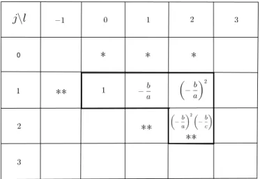
shown in Table 1, where the (j, l) entry in the boxed area is the Bohr-Fourier coefficient of ˜ϕ1+ corresponding to ejx−ly. The positions marked with∗ and
∗∗ correspond to the points in the spectra of ϕ2− and eλϕ2+ respectively.
Figure 1: Table 1
Thus we have, for Problem (g, r), ˜ ϕ1+ = ex− b aex−y+ b2 a2ex−2y− b3 a2ce2x−2y, (3.11)
which implies that the solution to Problem g is given by
ϕ1+ = ex+y−α− b aex−α+ b2 a2ex−y−α− b3 a2ce2x−y−α, (3.12) ϕ2+ = −a ex+y−λ+ b3 ace2x−y−λ+ b4 a2ce2x−2y−λ, (3.13) ϕ2− = c− bc a e−y+ b2c a2 e−2y, (3.14) if x− y ≥ α. (3.15)
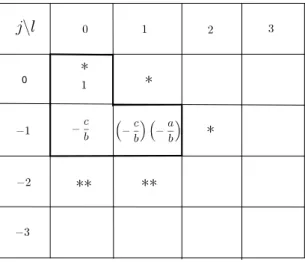
For x− y < α it is not possible to continue the same procedure and obtain a solution to Problem (g, r) satisfying (3.8). However, we can obtain a solution to Problem (g, v) for which (3.3) holds, according to the table below. The (j, l) entry in the boxed area there is the Bohr-Fourier coefficient of ϕ1−) corresponding to ejx−ly, while ∗ and ∗∗ correspond to the points in the spectra of e−α+yϕ2+ and e−λ−α+yϕ2− respectively. Note that 0 ∈
Figure 2: Table 2
Thus we have the following solution of the Problem (g, v):
ϕ1− = 1− c be−x+ ac b2e−x+y, (3.16) ϕ2− = − ac2 b2 e−2x+λ+α− c2 b e−2x−y+λ+α, (3.17) ϕ2+ = −beα−y− aeα− a2c b2 e−x+y+α. (3.18)
For the case when (3.9) and, in addition, (3.15) hold, we see from (3.12)– (3.13) that
(ϕ1+, ϕ2+) = eδ(ϕc1+, ϕc2+),
where
δ = min{x + y − λ, 2x − 2y − λ, x − y − α} (3.19) and ϕc1+, ϕc2+ ∈ AP P+.
On the other hand, as suggested by Table 1, we have ˜ ϕ1+= 1 cexϕ2−− b3 a2ce2x−2y
where ˜ϕ1+= eα−yϕ1+, which shows that
inf S ( |ϕc 1+| + |ϕc2+| ) > 0
for any strip of finite width parallel to the real axis (see the proof of Theorem 2.3 in [3]), while inf C+\S|ϕ1+| > 0 if δ = x + y − α, and inf C+\S|ϕ2+| > 0 if δ = x + y − λ or δ = 2x − 2y − λ.
Therefore (ϕc1+, ϕc2+) is a corona pair in C+, and we can see analogously that (ϕ1−, ϕ2−) is a corona pair in C−. Consequently, G admits an AP P
factorization with partial AP indices±δ defined by (3.19) [4, Theorem 3.8]. Similarly, if (3.9) holds and x− y ≤ α, the partial AP indices are ±δ with
δ = min{λ − x, α − y, α + y − x}.
We conclude, in particular, that an AP factorization of G, with x, y, α sat-isfying (3.9), is canonical if and only if
x + y = λ or x− y = α.
Indeed, for these values of x, y, α we always have α > y, 2x− 2y > λ,, while
x = λ if and only if x− y = α.
Finally, for x− y = α, (3.12)–(3.14) and (3.16)–(3.18) yield two linearly independent solutions of the Riemann-Hilbert problem (1.1) which define the factors
G± = [G±ij] (3.20)
in a canonical factorization (2.2) of G, where
G+11 = e2(x−α)− b aex−α+ b2 a2 − b3 a2cex G+12 = eλ− c beλ−x+ ac b2eλ−α G+21 = −a ex+y−λ+ b3 ace2x−y−λ+ b4 a2ce2x−2y−λ G+22 = −beα−y− aeα− a2c b2 G−11 = e2(x−α)−λ− b aex−α−λ+ b2 a2 e−λ− b3 a2cex−λ G−12 = 1−c be−x+ ac b2e−α G−21 = c−bc a e−y+ b2c a2 e−2y G−22 = −ac 2 b2 e−2x+λ+α− c2 b e−2x−y+λ+α.
4. Subgroup supported solutions to problem g: the trinomial case
Using the notation (3.7) introduced in Section 3, the conditions (3.5)–(3.6) imposed on sp(g) can be rewritten as
0 < y≤ α < λ, λ ≤ x + y < λ + α, x > 0, x
y ∈ Q/ (4.1)
and
x + y̸= λ or y ̸= α. (4.2) We defineP as the set of all triples (x, y, α) satisfying (4.1) and (4.2). From x + y≥ λ and y ≤ α it follows that x + α ≥ λ and, taking (4.2) into account, we have
x + α > λ. (4.3)
Below we will repeatedly use the standard notation [x] for the integer part of x∈ R, that is, the largest integer not exceeding x. On the other hand,
⌊x⌋ will stand for the largest integer strictly smaller than x: ⌊x⌋ =
{
[x] if x /∈ Z,
x− 1 otherwise.
Lemma 4.1. Let (x, y, α)∈ P. Then for all n ∈ Z we have either
[ λ + ny x ] = [ α + ny x ] , or [ λ + ny x ] = [ α + ny x ] + 1.
Proof. It is clear that, since α∈]0, λ[, we have α + ny x < λ + ny x , and so [ α + ny x ] ≤ [ λ + ny x ] . (4.4) From (4.3), λ + ny x < α + ny x + 1. (4.5) Since [ λ+ny x ]
For any (x, y, α)∈ P, let J1(x,y,α):= { j∈ N ∪ {0} : [ α + jy x ] = [ λ + jy x ] and λ + jy x ∈ N/ } and J(x,y,α) := { j∈ N ∪ {0} : [ α + jy x ] = ⌊ λ + jy x ⌋} .
To prove our next result, the one-dimensional version of Kronecker’s theorem will be needed, see e.g. [10]. For convenience of reference, we provide its statement below.
Theorem 4.2. Let p be a positive irrational number. Then the set {np −
[np] : n∈ N} is dense in the interval [0, 1].
Theorem 4.3. For all (x, y, α)∈ P, we have J1(x,y,α)̸= ∅.
Proof. If x + y > λ, according to Kronecker’s Theorem 4.2, there is some n∈ N ∪ {0} such that (n + 1)y x − [ (n + 1)y x ] < 1−λ− y x , (4.6)
since 0 < 1−λ−yx < 1. Thus we have λ + ny x = (n + 1)y x + λ− y x < 1 + [ (n + 1)y x ] ≤ 1 + [ α + ny x ] , so [ λ+ny x ]
< 1 +[α+nyx ]. Since λ+nyx > α+nyx , we cannot have λ+nyx ∈ N and therefore, by Lemma 4.1 we have
[ α + ny x ] = ⌊ λ + ny x ⌋ = [ λ + ny x ] .
If x + y = λ, from Kronecker’s Theorem we have that there is some n ∈ N ∪ {0} such that (n + 1)y x − [ (n + 1)y x ] > λ− α x ,
where 0 < λ−αx < 1. Since in this case (n+1)yx = λ+nyx , we have
λ + ny x − [ λ + ny x ] > λ− α x .
It follows that [
λ+ny x
]
< α+nyx . Therefore, we have [ λ+ny x ] = [α+nyx ] and λ+ny x ∈ N, so/ [α+ny x ] = ⌊ λ+ny x ⌋ .
If λ+nyx ∈ N, then λ+nyx − 1 ∈ N and x + y > λ. From (4.6) we have
λ + ny x − 1 < [ (n + 1)y x ] ≤ 1 + [ α + ny x ] ≤ 1 + [ λ + ny x ] = 1 + λ + ny x .
Therefore we must have [ (n + 1)y x ] = 1 + [ α + ny x ] = 1 + λ + ny x
and [α+nyx ]= λ+nyx , which is impossible because [α+nyx ]≤ α+nyx < λ+nyx .
Since J1(x,y,α) ⊂ J(x,y,α), we immediately conclude the following:
Corollary 4.4. For all (x, y, α)∈ P, we have J(x,y,α)̸= ∅.
Having fixed (x, y, α)∈ P, let now
N(x,y,α) := min J(x,y,α), (4.7)
S−1 = 1, (4.8) Sl = [ λ + ly x ] if l = 0, 1, . . . , N− 1, (4.9) SN := [ α + N y x ] = ⌊ λ + N y x ⌋ . (4.10) It is clear that λ + N y x − 1 ≤ SN ≤ α + N y x , (4.11)
and on the other hand we have
λ + ly x − 1 ≤ λ + ly x + α− y x − 1 ≤ α + ly x < λ + ly x , (4.12)
for all l∈ N ∪ {0}. So, the following theorem holds:
Theorem 4.5. For all (x, y, α)∈ P we have
α + ly x < Sl < λ + ly x and Sl = [ α + ly x ] + 1 for all l = 0, . . . , N− 1, (4.13)
(i) λ+N yx − 1 < SN ≤ λ+N yx +α−yx − 1 ,
(ii) λ+N yx + α−yx − 1 ≤ SN < α+N yx ,
(iii) SN = λ+N yx − 1 ,
(iv) SN = α+N yx .
Proof. By (4.7), (4.9) and (4.10) we cannot have Sl≤ α+lyx , since this would imply that λ+lyx ∈ N, because otherwise we would have S/ l = λ+lyx − 1 and ⌊ λ+ly x ⌋ = [ λ+ly x ] = [ α+ly x ]
, which is impossible for l < N . On the other hand, we have Sl ≤ λ+lyx but we cannot have Sl = λ+lyx since this would imply that ⌊ λ+ly x ⌋ = λ+lyx − 1 = [ α+ly x ]
, which is impossible for l < N . Therefore (4.13) must hold. The rest follows immediately from (4.11) and (4.12).
Remark that we have λ≤ λ + α − y ≤ α + x.
We can now present a solution to the Riemann-Hilbert problem (1.1). Recall that, by Theorem 4.5, either λ ≤ (SN + 1)x− Ny ≤ λ + α − y or
λ + α− y ≤ (SN+ 1)x− Ny ≤ α + x.
Theorem 4.6. For all (x, y, α) ∈ P, the Riemann-Hilbert problem (1.1)
admits an APP solution (ϕ+, ϕ−) such that 0 ∈ sp(ϕ2−) or 0 ∈ sp(ϕ1−).
Namely, if
λ≤ (SN + 1)x− Ny ≤ λ + α − y , (4.14)
then an AP P solution to the Riemann-Hilbert problem (1.1) is given by
ϕr1+ = N ∑ l=0 Sl ∑ j=Sl−1 ( −b c )j−1( −b a )l ejx−(l−1)y−α+ ( −b c )SN( −b a )N eγ,(4.15) where γ = (SN+ 1)x− (N − 1)y − α , (4.16) ϕr2+ = N∑−1 l=0 S∑l+1 j=Sl+1 −a ( −b c )j−1( −b a )l+1 ejx−ly−λ −b ( −b c )SN( −b a )N e(SN+1)x−Ny−λ+ S0 ∑ j=S−1 ac b ( −b c )j ejx+y−λ −a ( −b c )SN( −b a )N e(SN+1)x−(N−1)y−λ, (4.17)
ϕr1− = e−λϕr1+, (4.18) ϕr2− = N ∑ l=0 c ( −b c )Sl−1−1( −b a )l e(Sl−1−1)x−ly. (4.19) Respectively, if λ + α− y ≤ (SN + 1)x− Ny ≤ α + x , (4.20)
then an AP P solution to the Riemann-Hilbert problem (1.1) is given by
ϕv1− = 1 + N ∑ l=0 Sl ∑ j=Sl−1 ( −c b )j( −a b )l e−jx+ly, (4.21) ϕv2− = N ∑ l=0 c ( −c b )Sl( −a b )l eλ−(Sl+1)x+(l−1)y+α, (4.22) ϕv1+ = eλϕv1−, (4.23) ϕv2+ = −beα−y− aeα− a ( −c b )SN( −a b )N e−SNx+N y+α− − N ∑ l=0 S∑l−1 j=Sl−1 a ( −c b )j( −a b )l e−jx+ly+α. (4.24)
Note that in (4.21) we have 0∈ sp(ϕv1−), while 0∈ sp(ϕr2−) in (4.19). To prove Theorem 4.6 we use the following two results.
Lemma 4.7. Let (x, y, α) ∈ P, and let N and Sl be defined by (4.9) and (4.10), respectively. Then
(i) 0≤ Sl−1≤ Sl for all l∈ {0, 1, . . . , N};
(ii) If l ∈ {0, 1, . . . , N − 1}, then α − y < jx − ly < λ, for all j = Sl−1, . . . , Sl;
(iii) (Sl+ 1)x− ly ≥ λ , for all l ∈ {0, 1, . . . , N − 1};
(iv) (Sl−1− 1)x − ly ≤ 0 , for all l ∈ {0, 1, . . . , N}.
Proof. For l = 0, 1, . . . , N− 1, statement (i) follows immediately from (4.9),
and for l = N , if λ+N yx ∈ N, from (4.10). On the other hand, if/ λ+N yx ∈ N,
then SN = λ+N yx − 1 = λ+N y−xx and
SN−1 = [ λ + (N− 1)y x ] = [ SN+ 1− y x ] ≤ SN + 1− y x < SN+ 1.
Therefore, SN−1≤ SN.
To prove (ii), it suffices to show that
Sl−1x− ly > α − y , (4.25)
Slx− ly < λ (4.26) since, for j = Sl−1, . . . , Sl, we have
Sl−1x− ly ≤ jx − ly ≤ Slx− ly. Now, since l− 1 < N, we have from Theorem 4.5
α + ly
x < Sl < λ + ly
x , l = 0, . . . , N− 1
so that Sl−1 > α+(lx−1)y and Slx− ly < λ. Thus, (4.25) and (4.26) hold. In its turn, (iii) easily follows from the definition of Sl. The same is true for (iv), taking into account that λ− y ≤ x because x + y ≥ λ.
Theorem 4.8. Let (x, y, α)∈ P, and let N be defined by (4.7). If
λ≤ (SN + 1)x− Ny ≤ λ + α − y , (4.27)
then an AP P solution to Problem (g, r) is given by
˜ ϕr1+ = N ∑ l=0 Sl ∑ j=Sl−1 ( −b c )j−1( −b a )l ejx−ly + ( −b c )SN( −b a )N e(SN+1)x−Ny, ϕr2+ = N∑−1 l=0 S∑l+1 j=Sl+1 −a ( −b c )j−1( −b a )l+1 ejx−ly−λ+ −b ( −b c )SN( −b a )N e(SN+1)x−Ny−λ+ S0 ∑ j=S−1 ac b ( −b c )j ejx+y−λ −a ( −b c )SN( −b a )N e(SN+1)x−(N−1)y−λ, ˜ ϕr1− = e−λϕ1+, ϕr2− = N ∑ l=0 c ( −b c )Sl−1−1( −b a )l e(Sl−1−1)x−ly.
Proof. A straightforward computation shows that
(ce−x+ b + aey) ˜ϕr1+ = ϕr2−− eλϕr2+.
To prove that sp( ˜ϕr1+) ⊂ [α − y, λ + α − y], it suffices to show that for all
l = 0, . . . , N and j = Sl−1, . . . , Sl,
α− y ≤ jx − ly ≤ λ + α − y
and
α− y ≤ (SN + 1)x− Ny ≤ λ + α − y. (4.28) If l = 0, . . . , N− 1, from Lemma 4.7 (ii), we have
α− y < jx − ly ≤ λ ≤ λ + α − y,
for all j = Sl−1, . . . , Sl. If l = N , since
SN−1x− Ny ≤ jx − Ny ≤ SNx− Ny for j = Sl−1, . . . , Sl, it suffices to show that
SN−1x− Ny ≥ α − y and SNx− Ny ≤ λ + α − y,
which is indeed the case due to Lemma 4.7 and (4.27), respectively. On the other hand, it is easy to see from (4.27), that (4.28) holds.
It remains to prove that ϕr2±∈ H∞±. As to ϕr2+, we have:
• If l = 0, . . . , N − 1, we have (Sl+ 1)x− ly − λ ≤ jx − ly − λ, for all
j = Sl+ 1, . . . , Sl+1. But due to Lemma 4.7, (Sl+ 1)x− ly − λ ≥ 0.
• From (v) of the same lemma, it follows that (SN+ 1)x− Ny − λ ≥ 0.
• Taking into account that 0 ≤ x + y − λ ≤ jx + y − λ, for all j = S−1, . . . , S0 and (4.27), we conclude that ϕr2+∈ H∞+.
By (iv) of Lemma 4.7, we have (Sl−1− 1)x − ly ≤ 0, for all l = 0, . . . , N. So we conclude that ϕr2−∈ H∞−.
Proof of Theorem 4.6: Note that λ≤ λ + α − y ≤ α + x. So, according to
Theorem 4.5 we have either
λ≤ (SN+ 1)x− Ny ≤ λ + α − y (4.29) or
Let (4.29) hold. The Riemann-Hilbert problem (1.1) can be written in the
form {
e−λϕ1+ = ϕ1−
(ce−x+ b + aey)ϕ1+= ϕ2−− eλϕ2+
where ϕ1+ = eα−yϕ˜1+. Therefore, the Riemann-Hilbert problem (1.1)
ad-mits a solution ϕ1+ if and only if ˜ϕ1+ = e−α+yϕ1+ is a solution to Problem
(g, r). Therefore, the solution to (1.1) immediately follows from the above mentioned equivalence with Problem (g, r) and from Theorem 4.8; in this case 0∈ sp(ϕr2−).
Let (4.30) hold. We will prove now that
sp(ϕv1−)⊂ [−λ, 0] and ϕv2±∈ H∞±. • If l = 0, . . . , N, to prove that sp(ϕv 1−) ⊂ [−λ, 0], it is enough to show that −Slx + ly≥ −λ (4.31) −Sl−1x + ly≤ 0, (4.32) since, for j = Sl−1, . . . , Sl, we have
−Slx + ly≤ −jx + ly ≤ −Sl−1x + ly.
It is easy to see that (4.31) follows from Lemma 4.7 (v) and (vi). From (vi) of the same lemma we have−Sl−1x + (l− 1)y < −α , l = 0, . . . , N . Since y≤ α we have −Sl−1x + ly < y− α ≤ 0 and therefore (4.32) holds.
• To prove that ϕv
2− ∈ H∞−, we have to show that
λ− (Sl+ 1)x + (l− 1)y + α ≤ 0, for l = 0, . . . , N. (4.33) If l = 0, . . . , N− 1, taking into account that x + y ≥ λ and Lemma 4.7 (vi), we have
Slx− ly > α ≥ α + λ − x − y. (4.34) If l = N , from (4.30) we have also
(SN + 1)x− Ny ≥ λ + α − y. (4.35) So (4.34) and (4.35) imply (4.33) and we conclude that ϕv2−∈ H∞−.
• As to ϕv
2+, due to (4.30) we have that −SNx + N y + α ≥ 0, so it is clear that α−y, α, −SNx + N y + α≥ 0. Therefore, it remains to prove that −jx + ly − α ≥ 0, for all l = 0, . . . , N and j = Sl−1, . . . , Sl− 1. Since−jx + ly − α ≥ −(Sl− 1)x + ly − α, we just have to show that
−(Sl− 1)x + ly − α ≥ 0, for l = 0, . . . , N. (4.36) If l = 0, . . . , N− 1, taking into account that x ≥ λ − α and Lemma 4.7 (vi) we have
Slx− ly ≤ λ ≤ α + x. (4.37) If l = N , from (4.30) we have
SNx− Ny ≤ α < α + x. (4.38) Therefore from (4.37) and (4.38) we have (4.36) and we conclude that
ϕv2+ ∈ H∞+.
Finally, a straightforward computation shows that in fact (4.21)–(4.24) is an AP P solution to (1.1) with 0∈ sp(ϕv1−).
5. Partial AP indices and canonical factorization
As was already mentioned in Section 2, matrix functions (1.2) with g defined by (3.4)–(3.6) are AP P factorable. We will now use Theorem 4.6 to extract some additional information concerning the partial AP indices ±eδ of this factorization. To this end, observe the following:
(i) if λ≤ (SN+ 1)x− Ny ≤ λ + α − y, then: ϕ+= eδ ( ϕc1+, ϕc2+) with ϕc1+, ϕc2+∈ AP P+, δ = min ({δ1, δ2} ∪ {Slx− ly − α , l = 0, . . . , N − 1}) , (5.1) with δ1 = (SN + 1)x− Ny − λ , δ2 = x + y− λ; 0∈ sp(ϕc1+), 0∈ sp(ϕ2−). (ii) if λ + α− y ≤ (SN + 1)x− Ny ≤ α + x, then: ϕ+= eδ ( ϕc1+, ϕc2+) with ϕc1+, ϕc2+∈ AP P+, δ = min ({δ1, δ2} ∪ {λ − Slx + ly , l = 0, . . . , N− 1}) , (5.2) with δ1 =−SNx + N y + α , δ2 = α− y; 0∈ sp(ϕc2+), 0∈ sp(ϕ1−).
We now conclude:
Theorem 5.1. The partial AP indices ±δ of G are given by (5.1)–(5.2) if
(ϕc1+, ϕc2+) and (ϕ1−, ϕ2−) are corona pairs. In that case, δ≤ µ = α − y.
Recall that the Toeplitz operator TG with matrix n × n symbol G acts according to the formula
TGf = P+Gf, f ∈ Xn.
Various settings are possible, depending on the choice of the space X and the respective meaning of the (acting entry-wise) projection P+. In particular,
X may be a Hardy space H+
p of functions analytic in the upper half space with 1 < p < ∞; P+ is then the projection of Lp onto Hp+ parallel to
Hp−, and G can be any matrix function in Ln∞×n. For G ∈ APn×n one may also take X to be the Besicovitch space, and for G ∈ AP Wn×n the case X = AP W+ can be considered; see [2] for the detailed treatment. In all the settings mentioned above, the relation between certain properties of TG (Fredholmness, one- or two-sided invertibility, dimensions of kernel and cokernel, etc.) and an appropriate factorization of the symbol G are the same, and therefore we will not specify the spaces in the forthcoming statements.
Corollary 5.2. Let (x, y, α)∈ P and let N be defined by (4.7). A necessary
condition for TG to be invertible is that δ, given by (5.1)–(5.2) is equal to 0,
i.e.: (i) (SN + 1)x− Ny = λ, or x + y = λ, or SLx− Ly = α, for some L ∈ {0, . . . , N − 1}, if λ≤ (SN + 1)x− Ny ≤ λ + α − y (5.3) (ii) SNx− Ny = α, or y = α, or SLx− Ly = λ, for some L ∈ {0, . . . , N − 1}, if λ + α− y ≤ (SN + 1)x− Ny ≤ α + x. (5.4)
These conditions are necessary and sufficient if (ϕ1+, ϕ2+) and (ϕ1−, ϕ2−)
are corona pairs in C+ and C−, respectively.
These results yield some simple criteria for the invertibility of Toeplitz oper-ators TG. For example, we have the following, in the notation of the previous theorem.
Theorem 5.3. If (x, y, α) ∈ P and, for some n ∈ N, we have x = λn or x = n−1α ≥ λn, then TG is invertible.
Proof. Let x = λn with n ∈ N. Then n − 1 ≤ αx < n and we have N = 0,
since⌊λx⌋ = n − 1 =[αx], S0 = n− 1, and ϕ2−= c. Therefore (ϕ1−, ϕ2−) is a
corona pair inC−. On the other hand it is clear that (4.14) is satisfied and it follows from Theorem 4.6 and from Theorem 2.3 in [3] that (ϕr1+, ϕr2+), given by (4.15) and (4.17), is a corona pair inC+.
We can follow a similar reasoning if x = nα−1 ≥ λn. In this case 1 < αλ ≤ nn−1 and n− 1 < λx = λα(n− 1) ≤ n, so that we also have ⌊λx⌋ = n − 1 = αx and
N = 0, and (4.20) is satisfied.
The existence of a canonical factorization can also be proved by determining two linearly independent solutions to the Riemann-Hilbert problem (1.1) satisfying the conditions of the following theorem. In that case δ, given by (5.1)–(5.2), is 0 and (ϕ1±, ϕ2±) are corona pairs inC±, respectively.
Theorem 5.4 ([5]). Let ϕ1+, ψ1+ be solutions to Problem (1.1). Then G
admits a canonical bounded factorization (2.2) with
G− = [ ϕ1− ψ1− ϕ2− ψ2− ] , G+= [ ϕ1+ ψ1+ ϕ2+ ψ2+ ]−1 ,
if, for some sequence (ξn) such that ξn∈ C+ (respectively, C−) and |ξn| → +∞ we have
lim
n→∞(ϕ2+ψ1+− ψ2+ϕ1+)(ξn)̸= 0,
(respectively, limn→∞(ϕ2−ψ1−− ψ2−ϕ1−)(ξn)̸= 0). Now we have the following.
Theorem 5.5. Under the assumptions of Corollary 5.2, the necessary
con-ditions established in this corollary for TG to be invertible are also sufficient
if:
(i) (5.3) holds and
SLx− Ly = α, for some L ∈ {0, . . . , N − 1}, (5.5) or (SN + 1)x− Ny = λ, with N = 0 or ⌊ λ− α y ⌋ ≤ x− α y , (5.6) or x + y = λ.
(ii) (5.4) holds and SLx− Ly = λ, for some L ∈ {0, . . . , N − 1}, (5.7) or SNx− Ny = α, with ⌊ λ− α + y x ⌋ ≤ λ x − 1, (5.8) or y = α.
Proof. (i) Assume that (5.3) holds. If (5.5) or (5.6) hold, we see from Theorem 5.4 that TG is invertible, by taking ϕ1± = ϕr1±, ϕ2± = ϕr2±,
where ϕr1±, ϕr2± are defined by (4.15–4.19), and
ψ1− = 1 + L ∑ l=0 Sl ∑ j=Sl−1 ( −c b )j( −a b )l e−jx+ly, ψ2− = L ∑ l=0 c ( −c b )Sl( −a b )l eλ−(Sl+1)x+(l−1)y+α, ψ1+ = eλψ1−, ψ2+ = −beα−y− aeα− a ( −c b )SL( −a b )L − L ∑ l=0 S∑l−1 j=Sl−1 a ( −c b )j( −a b )l e−jx+ly+α if (5.5) is satisfied, and ψ1− = 1 + N ∑ l=0 Sl ∑ j=Sl−1 ( −c b )j( −a b )l e−jx+ly+ ( −c b )SN+1( −a b )N e−λ + k−1 ∑ j=1 ( −c b )SN+1( −a b )N +j e−λ+jy, ψ2− = N∑−1 l=0 c ( −c b )Sl( −a b )l eλ−(Sl+1)x+(l−1)y+α +c k−1 ∑ j=0 ( −c b )SN+1( −a b )N +j e−x+(j−1)y+α, ψ1+ = eλψ1−,
ψ2+ = −beα−y− aeα− a ( −c b )SN( −a b )N e−λ+x+α − N ∑ l=0 S∑l−1 j=Sl−1 a ( −c b )j( −a b )l e−jx+ly+α+ +b ( −c b )SN+1( −a b )N +k e−λ+(k−1)y+α, where k = ⌊ λ− α y ⌋ + 2, if (5.6) is satisfied.
Note that x + y = α + σ, so the case x + y = λ is covered by [14]. (ii) Assume now that (5.4) holds. Then, if (5.7) or (5.8) holds, we conclude
from Theorem 5.4 that TG is invertible by taking ϕ1± = ϕv1±, ϕ2± =
ϕv2±, where ϕv1±, ϕv2± are defined by (4.21)–(4.24), and
ψ1+ = L ∑ l=0 Sl ∑ j=Sl−1 ( −b c )j−1( −b a )l ejx−(l−1)y−α+ ( −b c )SL( −b a )L ex+y−α, ψ2+ = L−1 ∑ l=0 S∑l+1 j=Sl+1 −c ( −b c )j( −b a )l ejx−ly−λ− b ( −b c )SL( −b a )L − S0 ∑ j=S−1 a ( −b c )j−1 ejx+y−λ− a ( −b c )SL( −b a )L ey, ψ1− = e−λψ1+, ψ2− = L ∑ l=0 c ( −b c )Sl−1−1( −b a )l e(Sl−1−1)x−ly. if (5.7) is satisfied, and ψ1+ = N ∑ l=0 Sl ∑ j=Sl−1 ( −b c )j−1( −b a )l ejx−(l−1)y−α+ ( −b c )SN−1( −b a )N +1 + k ∑ j=1 ( −b c )SN+j−1( −b a )N +1 ejx,
ψ2+ = N∑−1 l=0 S∑l+1 j=Sl+1 −a ( −b c )j−1( −b a )l+1 ejx−ly−λ − S0 ∑ j=S−1 a ( −b c )j−1 ejx+y−λ−bc a ( −b c )SN+k( −b a )N eα−y+kx−λ − k ∑ j=1 a ( −b c )SN+j−1( −b a )N +1 eα+jx−λ, ψ1− = e−λψ1+, ψ2− = c2 a ( −b c )SN( −b a )N eα−y−x− N ∑ l=0 c2 b ( −b c )Sl−1( −b a )l e(Sl−1−1)x−ly, if (5.8) is satisfied, where k = ⌊ λ−α+y x ⌋ + 1.
If y = α, that is, µ = 0, the operator TG is invertible by [5].
The proof of Theorem 5.5 provides an explicit canonical factorization for G, revealing in particular additional information concerning the Bohr-Fourier spectra of the entries of G±. To put this in perspective, recall that according to [19] for any G admitting an AP factorization and such that sp(G)⊂ Σ for some additive subgroup of R, it is possible to choose a factorization in such a way that
sp(G±), sp(G−1± )⊂ Σ. (5.9) In particular, the partial AP indices of G lie in Σ. If the AP factorization of
G is a priori canonical, the latter statement is redundant, and the property
(5.9) holds for every factorization of G, as was shown earlier in [1, 20]. For matrix functions (1.2) this observation was strengthened in [6]. Skipping technical details, for which we refer to Theorem 6.1 of [6], the result is as follows: if sp(g) ⊂ Σ0 for some subgroup Σ0 of R and (1.2) admits a
canonical factorization, then each entry of G± (and thus G−1± as well) has its Bohr-Fourier spectra located in exactly one of the three sets Σ0, Σ0+ λ
and Σ0−λ. In our setting of g given by (1.5), Σ0= xZ+yZ+αZ. However,
the formulas obtained while proving Theorem 5.5 show that in fact the Boh-Fourier spectra of each entry of G±, G−1± belong to one of five smaller sets Σ1, Σ1± α, Σ1± (α + λ), where Σ1 is the subgroup xZ + yZ of Σ0.
Remark 5.6. It remains to be seen whether an AP P factorization of G is
N = 0 or ⌊ λ−α y ⌋ ≤ x−α
y , and when (5.4) and (5.8) hold without the
addi-tional condition that
⌊ λ−α+y
x ⌋
≤ λ
x−1. The authors’ conjecture is that, in all
cases, the necessary conditions of Corollary 5.2 are sufficient for invertibility of TG.
6. Example
Assume now that α, µ, σ are such that (3.5) holds, and in addition
α > 2
3λ ,
λ
2 ≤ x ≤ λ, (6.1)
with x defined by (3.7). From the results of Section 4, it follows that:
Theorem 6.1. For all (x, y, α)∈ P satisfying (6.1), the Riemann-Hilbert
problem (1.1) admits an AP P solution (ϕ+, ϕ−) given by
ϕ1+ = 1 cex+y−α(1− η) ϕ2−+ ζ, (6.2) ϕ2+ = −e−λP[0,+∞[(gϕ1+), (6.3) ϕ1− = e−λϕ1+, (6.4) where (I) if λ≤ 2x ≤ α + x, we have (i) ϕ2−= c, η = 0, ζ =− b ce2x+y−α, if 2x≤ λ + α − y; (ii) ϕ2−= c ( −c b ) eλ+α−2x−y, η = 0, ζ = eλ, if 2x≥ λ + α − y; (II) if α≤ x ≤ α + y, we have (i) ϕ2−= c− c k−1 ∑ j=0 ( b a )j+1( b c )j ejx−(j+1)y, η = b cex, ζ = b ce2x+y−α, if λ≤ (k + 1)x − ky ≤ λ + α − y, k∈ N ;
(ii) ϕ2−= c (a b )k(c b )k eλ+α−(k+1)x+(k−1)y − k−1 ∑ j=0 c (a b )j(c b )j+1 eλ+α−(j+2)x+(j−1)y, η = b cex, ζ = (a b )k(c b ) eλ−(k−1)x+ky, if λ + α− y ≤ (k + 1)x − ky ≤ λ + x − y, k∈ N; (III) if α + y≤ x, we have (i) ϕ2−= k+1 ∑ j=0 c ( −b a )j e−jy, η = 0, ζ = ( −b a )k+1( −b c ) e2x−ky−α, if α + x− y ≤ 2x − (k + 1)y ≤ λ + α − y, k∈ N; (ii) ϕ2−= k+1 ∑ j=0 c ( −a b )j( −c b ) eλ+α−2x+(j−1)y, η = 0, ζ = eλ, if λ + α− y ≤ 2x − (k + 1)y ≤ α + x, k∈ N.
Theorem 6.2. For all (x, y, α)∈ P satisfying (6.1), the partial AP indices
±δ of G are given by the following formulas (I) if λ≤ 2x ≤ α + x, we have
(i) δ = min{2x − λ, x + y − λ}, if 2x≤ λ + α − y;
(ii) δ = min{α − x, α − y}, if 2x≥ λ + α − y;
(II) if α≤ x ≤ α + y, we have
(i) δ = min{(k + 1)x − ky − λ, x − α},
if λ≤ (k + 1)x − ky ≤ λ + α − y, k∈ N ; (ii) δ = min{λ − kx + (k − 1)y, α − y, α − k(x − y)},
if λ + α− y ≤ (k + 1)x − ky ≤ λ + x − y, k∈ N; (III) if α + y≤ x, we have
(i) δ = min{x − ky − α, x + y − λ},
if α + x− y ≤ 2x − (k + 1)y ≤ λ + α − y, k∈ N; (ii) δ = min{λ − x, α + (k − 1)y − x},
if λ + α− y ≤ 2x − (k + 1)y ≤ α + x, k∈ N.
Proof. We prove this result for the case (I)-(i); in the remaining cases the
proof is similar, using (6.2) and Theorem 2.3 in [3].
Let λ≤ 2x ≤ α + x and 2x ≤ λ + α − y. Then from (6.2)–(6.4) we obtain
ϕ1+ = ex+y−α+ ( −b c ) e2x+y−α, ϕ2+ = a ( −b c ) ( −b a ) e2x−λ− aex+y−λ− a ( −b c ) e2x+y−λ, ϕ1− = e−λϕ1+, ϕ2− = c .
It is easy to check that (ϕ1+, ϕ2+) = eδ(ϕc1+, ϕc2+), where δ = min{2x −
λ, x + y− λ} and ϕc1+, ϕc2+∈ AP P+. Moreover, by (6.2) we have inf
S (|ϕ c
1+| + |ϕc2+|) > 0
for any strip S of finite width parallel to the real axis (see the proof of Theorem 2.3 in [3]). In addition, infC+\S|ϕc2+| > 0 if δ = 2x − λ or δ =
x+y−λ. Therefore (ϕc
1+, ϕc2+) is a corona pair inC+. We can see analogously
that (ϕ1−, ϕ2−) is a corona pair inC−, since infS(|ϕ1−| + |ϕ2−|) > 0 for any
strip S as above and infC−\S|ϕc2−| > 0 (cf. [3, Theorem 2.3]).
From here we immediately obtain:
Corollary 6.3. For (x, y, α)∈ P satisfying (6.1), we have 0 ≤ δ ≤ µ.
Note that we may have δ = µ, and therefore Corollary 6.3 provides optimal estimate for the partial AP indices.
Corollary 6.4. Let (x, y, α)∈ P satisfy (6.1). A necessary and sufficient
condition for TG to be invertible is that
(I) if λ≤ 2x ≤ α + x, we have
(i) x = λ2 or x + y = λ, if 2x≤ λ + α − y;
(II) if α≤ x ≤ α + y, we have (i) (k + 1)x− ky = λ or x = α, if λ≤ (k + 1)x − ky ≤ λ + α − y, k ∈ N ; (ii) kx− (k − 1)y = λ or k(x− y) = α, if λ + α− y ≤ (k + 1)x − ky ≤ λ + x − y, k∈ N; (III) if α + y≤ x, we have (i) x− ky = α or x + y = λ, if α + x− y ≤ 2x − (k + 1)y ≤ λ + α − y, k∈ N; (ii) x = λ or x− (k + 1)y = α, if λ + α− y ≤ 2x − (k + 1)y ≤ α + x, k∈ N.
The factors in a canonical factorization of G can be obtained, for λ2 < x < λ, x + y > λ, from Theorem 6.1 noting that, in each case, it provides two
linearly independent solutions to Problem g. Thus, for instance, if x−y = α, then (6.2)–(6.4) and (II)-(i) provide the first columns of G+ and G−, while
(6.2) – (6.4) and (III)-(ii) provide the second columns of these factors (cf. (3.20)).
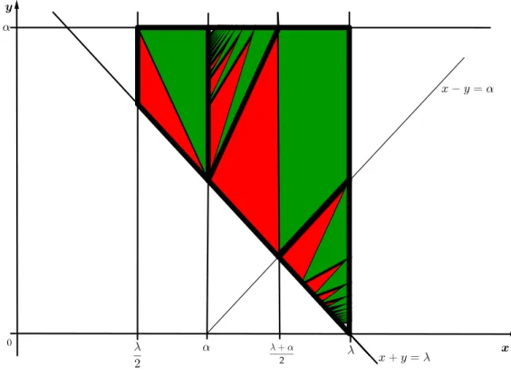
In Figure 3 we represent the cross-section ofP satisfying (6.1) for a certain value α (α = 0, 67) indicating by different colours the points corresponding to (I)-(i), (II)-(i), (III)-(i) (red) and to (I)-(ii), (II)-(ii), (III)-(ii) (green). (In the black and white version red and green correspond to dark and light grey, respectively.) The points on the thicker black lines are those corresponding to values of (x, y, α) for which G admits a canonical factorization, accord-ing to Corollary 6.4. For all other points the results of Theorems 6.1 and 6.2 provide an explicit solution to Problem g and to the Riemann-Hilbert problem (1.1), as well as explicit formulas for the partial AP indices. It may be worth noting that the borderline cases α + σ = λ and α + σ > λ,
µ = 0 for which explicit necessary and sufficient conditions for existence of a
canonical factorization of G were previously known, as mentioned in Section 1, correspond only to the boundary lines of the polygon which are given by the equations x + y = λ, y = α in the (x, y) plane.
7. Final remarks
7.1. More general AP polynomials
The table method approach is by no means exhausted by the class of symbols studied in the previous sections. The following examples illustrate this point.
Figure 3: Cross-section for α = 0, 67.
Example 7.1 Assume that
g = c e−x+ b + a ey+ d e2y
with a, b, c, d∈ C\{0}, x, y, α for which (3.10) holds and α > 23λ.
Analogously to what was done in Tables 1 and 2 in Section 3, we see that a solution to Problem g, and to the Riemann-Hilbert problem (1.1), is given by ϕ1+ = ex+y−α− ab bd− a2ex−α− b2 bd− a2ex−y−α − b3 bdc− a2ce2x−y−α, (7.1)
ϕ2+ = ( −a − abd bd− a2 ) ex+y−λ− ab3 bdc− a2 e2x−y−λ + b 4 bdc− a2ce2x−2y−λ− dex+2y−λ− db3 bcd− a2ce2x−λ, (7.2) ϕ2− = c + abc bd− a2 e−y− b2c bd− a2e−2y, (7.3) if x− y ≥ α, and ϕ1− = 1− c be−x+ ac b2e−x+y, (7.4) ϕ2− = − ac2 b2 e−2x+λ+α− c2 b e−2x−y+λ+α, (7.5) ϕ2+ = −beα−y− aeα− a2c− bcd b2 e−x+y+α −dey+α− acd b2 e−x+2y+α, (7.6) if x− y < α.
For x− y = α, (7.1)–(7.3) and (7.4)–(7.6) yield two linearly independent so-lutions of Gϕ+= ϕ−which define the factors G±in a canonical factorization
of G.
Example 7.2 Let now
g = c e−x+ b + a ey+ d ex−y
with a, b, c, d∈ C\{0}, x, y, α satisfying (3.10), and α > 23λ.
In this case a solution to Problem g is given by
ϕ1+ = ex+y−α− b aex−α+ b2 a2ex−y−α− b3 a2ce2x−y−α, (7.7) ϕ2+ = −a ex+y−λ− ( b3 ac− d ) e2x−y−λ+ b4 a2ce2x−2y−λ −bd ae2x−2y−λ− db2 a2 e2x−3y−λ+ db3 a2ce3x−3y−λ, (7.8) ϕ2− = c− bc a e−y+ b2c a2 e−2y (7.9) if x− y ≥ α, and
ϕ1− = 1− c be−x+ ac b2e−x+y, (7.10) ϕ2− = − ac2 b2 e−2x+λ+α− c2 be−2x−y+λ+α, (7.11) ϕ2+ = − ( b + dac b2 ) eα−y− aeα− a2c b2 e−x+y+α −dex−2y+α+ cd b eα−2y, (7.12) if x− y < α and y < α2.
For x− y = α, (7.7)–(7.9) and (7.10)–(7.12) yield two linearly independent solutions of Gϕ+= ϕ− which define the factors G± in a canonical
factoriza-tion of G.
These examples raise several interesting questions such as the following. Can the table method be applied to obtain solutions to the Riemann-Hilbert problem (1.1), with G given by (1.2), for any APP g? Is there always an
AP P solution to that Riemann-Hilbert problem? What are the optimal
solutions with respect to the Bohr-Fourier spectrum, and the best estimate of the partial AP indices in terms of the spectrum of g?
7.2. Non-AP symbols
Finally, we see that knowing the explicit expressions of the solutions to Problem g enables one to extend the results to some cases where the constant coefficients of the exponentials in g are replaced by functions, not even necessarily belonging to AP . To illustrate this point, note for example that in case (I) of Theorem 6.1 a bounded factorization of G exists, and exactly the same factorization formulas persist, when a constant coefficient a is replaced by an arbitrary function a∈ H∞+. This factorization is in fact AP ,
AP W , or AP P if and only if a belongs respectively to AP+, AP W+, or
AP P+.
Acknowledgments
The work of the first two authors on this paper was partially supported by Funda¸c˜ao para a Ciˆencia e a Tecnologia (FCT/Portugal), through Projects PTDC/MAT/121837/2010, PTDC/MAT-ANA/6126/2014 and