1
A Work Project, presented as part of the requirements for the Award of a Master Degree in
Finance from NOVA – School of Business and Economics
EUROPEAN INDUSTRY SEGMENTATION: A SIMPLE FACTOR INVESTING STRATEGY
RODRIGO BERNARDINO (30456)
A Project carried out on the Master in Finance Program, under supervision of:
João Pedro Pereira
2
Abstract
This report assesses a possible European industry segmentation (small and medium size
companies) through fundamental indicators, aiming to develop indicator-based strategies that
outperform the market, providing to the average investor a simple and efficient investment strategy.
According to its outcomes, all the constructed portfolios based on the indicator that provided the
maximum sharpe ratio, surpass its industry proxy and produced competitive results when compared
with the market. Its out-of-sample performance sustains our findings for almost all industries,
proving that this procedure can be a source of value for investment practices. This process can be
applied to other indicators or markets.
3
1. Introduction
Financial players are continuously looking for the optimization, efficiency improvement and return
maximization of their invested capital. Researchers look constantly for new tactical and strategical
approaches or new investment guidelines, leading investors to change or tilt their investments
according to these new findings. Asset management industry is thus also changing in response to
these new trends, turning more focused on risk-based asset allocation and on factor investing.
Factor-based investment is a rising theme in the last years, being used as an attempt to construct
more competent and better risk-managed portfolios. According to Blitz (2015), we can define three
sources of return: exposure to the market risk premium, to known factor premiums or alphas
(managerial skill). Risk factors are defined as a driver of asset returns which is related to a specific
characteristic of a security and associated with an inherent risk premium (which can be positive or
negative). Thus, a factor-based investment framework tries to identify factors that an investor
should be exposed to capture their risk premium, and consequently outperform the market: this
approach also allows investors to design their customized investment strategies by being exposed
and tilted on preferred factors (Yury Polyakov (2016) and Kees G. Koedijk, Alfred M.H. Slager &
Philip A. Stork (2016)). These concepts have been discussed and applied across the world,
especially under smart betas approaches context – a strategy which aims to offer exposure to factors
that persistently drive returns.
Based on this trend and discussion, this report aims to assess if it is to possible segment
European industries through its characteristics, looking for a simple investment strategy based in
factor investing approaches – through simple fundamental ratios and indicators – that can be used
for all the investors in the market. Its main goal is to assess if it is possible to identify industries
4
related literature topics and in section III it is explained the used methodology. Section IV to VI
discuss the main results and conclusions, providing a recommendation for the investors.
2. Literature Review
Factor investing has been implicitly present in the industry from a long time ago. In the 50s and
60s decades, several authors identified and developed models where returns were a function of the
market factor: the CAPM model, being later used as basis to develop the APT model where returns
were explained by a combination of n factors. Later, Fama and French (1992) raised a model where
size and value were relevant factors to explain asset returns, that was expanded by Carhart (1997)
based on Jegadeesh and Titman (1993) findings, being widely used to explain returns for a long
time in history. This incessant pursuit for relevant factors in order to identify how returns are built
and explained didn’t stop: the recent literature, shown us that authors are identifying more and
more factors that can be a good explanation for this question: up to now, were identified more than
300 factors that are supposed to deliver excess return (Harvey & Liu, 2014). According to Cazalet
& Roncalli (2014) and Hsu, Kalesnik & Viswanathan (2015), most of the identified and tested
factors are not significant. Every time that researchers identify some factors or patterns that provide
non-predicted returns by the pricing models they are assumed to be alphas, and consequently called
by anomalies. Yet, not all these “anomalies” are reliable or robust enough to drive investment
strategies: most of them, just as factors, might derive of data mining, market bias or simply noise,
and even when properly identified and tested, their benefits might not surpass the eventual costs
that investors need to incur to be exposed to it. Other important risks associated with anomalies are
their destruction after publications, once investors learn with market mispricing and exploit these
5
Even being not consensual, the factor concept is usually associated with several requirements
and characteristics: has extensive available historical data, survived to extreme events, was
extensively tested and replicated in numerous tests and different data sets, offers a persistent
premium and has a credible explanation (Jason Hsu & Vitali Kalesnik, 2014). Ang (2014) identified
two types of factors: macro (fundamental-based) and investment-style factors. The first group
includes factors such as economic growth, productivity, volatility and demographic risk; the
second, also exploited by Blitz (2016), includes market factors (as the used in CAPM), quality,
value, low risk and momentum factors. Ang (2014) defended that the two factors are linked, being
macro factors often reflected in the performance of investment factor, arguing that this relation is
quite intuitive, once if, for example, economic growth slows and inflation rises, firms and investors
are affected and the market prices will reflect this impact (see also Chen, Roll & Ross (1986)).
“Factors are to assets, what nutrients are to food” – Ang (2014) explains the factor theory based on the belief that factors represent a risk exposure, and consequently they deliver return.
Each factor is assumed to represent a different characteristic and consequently a different risk,
rewarding investors with different premium levels – premiums that change across the time
depending on the conjecture that surrounds the factor. Ceteris paribus, if a factor has a positive
risk premium, the higher the exposure to the factor, the higher the expected return of the underlying
asset. This line of thought can be both extrapolated to CAPM (market factor), or to multifactor
models. Once factors deliver returns, they can be a good source of profit for investors: in fact,
investment strategies based on these evidences, usually known as factor investing strategies, aim
to exposure a portfolio to certain characteristics: instead of diversifying across the entire market,
factor investors tilting their investments to certain factors depending on the targeted investment
6
what Fama and French (1992 and 1996) tested in the 90s, concluding that certain factors create
value: as mentioned by these authors, factor investing emerged as the byproduct of factor models
of asset pricing, due to the constant source of anomalies and extraordinary returns (see also Marie
Brière & Ariane Szafarz (2015). Factor investing is also consistent with CAPM theory, which
defends that investors should hold a factor (the market factor) instead of individual stocks:
individual stocks carry implicitly idiosyncratic risk that is not rewarded by a risk premium.
The main question of factor investing is related to the selection of the factors. Ang (2014),
defended that each investor demands a different amount and style of exposure, depending on its
characteristics as a market player: ”each individual investor has a different amount of factor
exposure just as different individuals have different nutrient requirements” (see also Hsu, Kalesnik
& Viswanathan (2015)). Therefore, the selection of the factors might be a problem for the average
investors: risk aversion level, long-term horizon, its utility curves, its capacity to afford big losses,
etc. are difficult measurement vectors. The number of factors to be exposed is also a key issue:
researches identified a vast list of factors, but most of them are not significant or robust. How can
they define an exact number? Investors should keep it simple, starting with a select few: Fama and
French (2015) told us that the marginal return improvement tends to decrease with the adding of
factors once the additional factor is probably positively correlated to the ones already included.
The amount of losses during bad periods is also an important issue for these strategies: Ang (2014)
identifies huge losses for value, volatility and momentum factors in the financial crisis over
2007-08, defending that factors are historically riskier in these bad phases, being factor premium
existence, in the long run, a compensation for the investor for bearing these losses. Still, historical
data and performance of these investments shown us that invest through factor vectors can bring
7
investors should also consider other additional benefits of its usage. The convenience provided is
one pertinent example: investors who hold a vast number of securities are normally investing based
on factors, tilting their portfolios according to their own criteria, instead of using a large-scale stock
picking strategy. The historically higher return level and the risk reduction – factor investing
portfolios are historically better risk managed – over longer periods, are other associated benefits.
In 1996, Robert A. Haugen and Nardin L. Baker tested and studied how firms’ characteristics
impact in expected returns – liquidity of its stocks, price assessment, potential growth, etc. Factors
are usually linked to firm characteristics due to logical issues: it is expected that firms’
characteristics affect their performance and market opinion. Their fundamentals, capital structure
or performance levels are common characteristics that allow its characterization, being their
analysis frequently associated to a potential power of predictability in future performance (and
returns), constituting a relevant subject for investors and researchers. Features such as
book-to-market, market capitalization, assets growth or dividend yield are examples of characteristics that
are historically related to average returns on common stocks, providing also a robust evidence of
being good descriptors of future returns (Fama & French (1996) and Lewellen (2014)). For
example, value factor is often described through firms’ book-to-market ratio, earnings yield or
dividend yield; debt-to-assets ratio, ROE or assets turnover ratio are usually good proxies for the
quality factor; low-risk factors are normally based on the historical volatility or betas; etc.
As firms, industries also have their own characteristics. Most of the time, firms’ characteristics
are highly correlated with the industry: within the same industry having, usually, a similar capital
structure, competing in the same markets, being subject to the same regulation and react similarly
to macroeconomic shocks, companies tend to be highly correlated (Tobias J. Moskowitz & Mark
8
segment them through factors, by identifying characteristics or fundamental indicators that explain
returns, and tilting our investments towards these vectors? Is it possible to invest in an industry
based on the same principles of factor investing? Is it possible to outperform the market based on
this characteristic based segmentation? That’s the questions that we will try to answer.
3. Data and Methodology
This section describes the data and methodology of the study, starting by describing the selected
data and its treatment, being followed by the explanation of the used procedures in the model
development and the assumptions made – transversal to all the studied industries. The model
includes an in-sample analysis, where are defined the indicators that will guide the investment
proposals, being later tested in an out-of-sample period. Finally, to the designed portfolios, will be
incorporated transaction costs effects aiming to provide a more realistic view of their performance.
3.1. Data Selection
All data was collected from Bloomberg L.P. and Kenneth R. French – Data Library. Bloomberg
identifies 11 sector industries: industrials, materials, informational technologies (IT), energy,
healthcare, communication services, consumer discretionary, financials, consumer staples, real
estate and utilities. Within each industry, was downloaded the monthly data of each constituent
company for the identified indicators, from February 1992 to September 2018.
Based on the objectives of this report, was created a filter that excluded companies with an
average market capitalization equal or above 30 Billion in the last 12 months of the sample. In the
technology and materials sectors were also not considered ADYEN N.V. and LIN GY Equity
respectively due to its recent IPO and consequent lack of available data (13th of June of 2018 and
9
end up with 251. For each company on each industry were downloaded the data for the following
ten indicators: current market capitalization, price-earnings ratio, dividend payout ratio, net
Debt/EBITDA, free cash flow yield, capex/sales, EBITDA/revenue, normalized ROE, adjusted
revenue growth (5 years) and sales growth, which were collected with the objective of reflecting
information of its pricing in the market, its cash flow and returns generation, its revenue and sales
evolution and its relation between performance and capital structure. The aggregated historical data
of each industry was downloaded through its Bloomberg index (see Appendix A).
To assess the potential alpha creation, the created portfolios in-sample were regressed against
the 3-Factors Fama-French model. The Kenneth R. French–Data Library provided monthly data
for market, SMB and HML factors and for the risk-free rate. For consistence issues, the provided
market and risk-free rate data were assumed as proxies for other required calculations.
3.2. Model Development
The model was applied to all the identified industries, allowing us to test and assess the
performance of a simple industry segmentation through fundamental indicators. Used procedure:
1) Indicator variation (including individual prices of each security);
2) Assessment of the correlation between price changes and indicator change;
3) Raking of the securities, per indicator, based on its correlation assessed in 2):
a. Indicators with positive or null correlation are ranked in a descending way;
b. Indicators with negative correlation are ranked in an ascending way;
4) Define the position on the different stocks according to its raking:
a. It is predefined a number of stocks (m) to invest in each industry, through the
10
b. The model provides two different outputs of positions:
i. Long-only strategy – portfolio holds a long position in m securities;
ii. Long-short strategy – portfolio holds a long position in m securities and a
short position in another m securities;
5) Construction of the portfolios based on the defined positions: each security’s position is
multiplied by its return, and this individual return is summed providing the monthly return
of the portfolio (equal-weighted portfolio). Everything was properly lagged;
6) Performance analysis of each constructed portfolio based on the different indicators. This
analysis is based in the first and second moments (annual return and standard deviation),
extending this analysis to higher moments providing a more complete and wider analysis.
Other relevant metrics are presenting here;
7) Construction, for the same sample, traditional investment portfolios to compare the
developed ones with most common investment strategies and assess the added value of this
strategy. As traditional investment strategies were considered investment portfolios such as
EW portfolio, a Momentum portfolio based on price changes (the number of long and short
securities stills constant (m)), a risk-parity approach and an inverse volatility portfolio;
8) Construction of long-only portfolios for the market and industry proxies.
3.2.1. In-sample Analysis
To provide a more reliable and robust analysis the model considers an in-sample analysis, where
the model assesses the performance of the designed portfolios from February 1992 to September
2016, and an out-of-sample analysis. All the portfolios are compared with the market and industry
portfolios, beyond the comparison with the identified traditional investment strategies. The model
11
1) Maximum average annual return: aims to provide a proxy for investors with a risk lover
profile, who focus their investment mainly based on potential and historical returns;
2) Minimum average annual standard deviation (only among the indicators that provided a
positive SR): intents to be a good approximation for risk-averse profile investors who, more
than high return levels, aim to reduce their potential loss risk;
3) Maximum Sharpe Ratio (SR): something in between the two above. Even though might not
be a good proxy an intermediate risk aversion level, the SR compares the level of return per
unit of volatility (a proxy for risk), which is believed to be a more rational indicator for the
average investor – based on this belief, this portfolio will be the base case for this analysis.
Besides that, it will be constructed two additional portfolios: firstly, a composite portfolio that
combines in equal proportions the three above selected, with the main objective of assessing if the
addition of characteristics adds value or not. Secondly, this latest composite portfolio will be
combined with a risk-management strategy (a risk-parity portfolio) in three different scenarios: the
first one with 35% weight on the risk-parity portfolio and the second and third ones with 50% and
65% respectively. The main goal here is to assess if risk-management strategies deliver value for
the investor and how its weights impacts on the portfolio performance. All the portfolios were also
analysed in terms of skew and kurtosis to provide a more complete and critical analysis.
3.2.2. Out-of-sample Analysis
In this analysis the indicator that provided the maximum SR portfolio, identified in the in-sample
analysis, the composite and risk-averse strategies were tested for the last 24 months of the collected
data sample (from October 2016 to September 2018). The main objective is to test if the
conclusions in-sample, produce or no positive results out-of-sample. The performance of the
12
3.3.3. Transaction costs incorporation
According to Korajczyk and Sadka, (2004), transaction costs are an important variable in
investment strategies development, which may turn apparently highly profitable portfolio on
extreme losses – they reduce the total return of the portfolio by increasing its total amount of costs.
To analyse them, and keeping the same line of thought, it will be introduced to the base case
portfolio a fixed amount of 0.15% for transaction costs (buy and sell costs are assumed to be the
same). In its consideration, it is counted the number of switches in each security position and
calculated the impact on the portfolio performance – the higher the number of switches, the higher
number of transactions, and consequently the higher transaction costs impact.
4. Results and Discussion
This section analyses the obtained results and discusses other important dimensions in the
developed strategies. To provide a more intuitive analysis, this assessment will be focused in
relevant evidences in each point in time, and based in a long-only approach, being the remaining
facts similarly analysed but in a more general way – all the outcomes of the test are properly
provided along this report. The analysis will be also mainly focused in the identified SR indicator
– it assumed to be the most rational and close to reality vector among the defined ones. 4.1. Long-only versus Long-short approach
Based on the maximum SR among the designed strategies, the selection of the indicator that drives
the investment strategy seems to not change depending on the defined approach: 8 out of 11
industries did not change their vector when using a long-short instead long-only method (Appendix
B). For the maximum annual average return and minimum annual standard deviation portfolios,
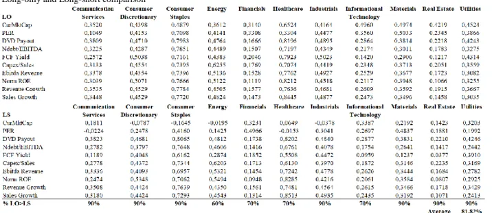
13 Table 1 – Obtained SR for each industry, based on the defined indicators (maximum SR approach) Long-only and Long-short comparison
their base indicator when vary across long-only and long-short approach. Looking to a wider point
of view, when the 10 indicators are compared among the 11 different industries based on the
maximum SR, we can see that on average, 81,82% of the times, long-only method provide better
results in terms of SR (see Table 1).
Another important issue is related to the amount of transaction costs and brokerage fees that
both methods require: long-short strategies are normally associated with higher levels of exposure
and consequently to higher risk. Market players are concerned about their exposure, and most of
the time they focus their investment mainly in long-only approaches (Blitz, Huij, Lansdorp, and
Vliet, (2014)). As mentioned before, long-only can provide a competitive outcome when compared
with long-short strategies, even not considering these accrual risks. The impact of transaction costs
will be later analysed and briefly discussed the impact of other associated costs.
4.2. Developed strategies versus traditional investment approaches – in-sample analysis
The obtained results in this comparison show us that, in terms of SR results, risk-management
14 Table 2 – SR levels for traditional and developed (LO and LS) strategies for the defined sample (maximum SR approach)
sectors (long-only designed strategy) are the exceptions to this evidence. As shown in Table 2,
even with lower SR, all the developed strategies provide competitive outcomes compared with
risk-management and surpassing most of the time EW and momentum outcomes.
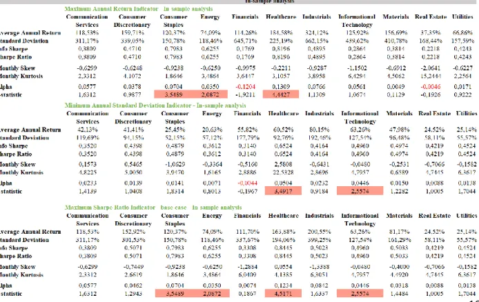
Table 3 summarizes the performance output of the different strategies in-sample. Based on the
defined proxies for risk aversion levels, most of the strategies produce positive and significant
results when compared with the 3-factor Fama-French model: the financial sector is the only
exception to this alpha positiveness at 5% confidence level – being this evidence only eliminated
when the investment portfolio is constructed according to the maximum SR indicator. A special
highlight for the industrials sector, that produces the highest significant alpha (0,0842). For the
maximum SR based approach – the base case approach – when compared with the benchmarks, it
is observed that all the industries surpass its respective industry benchmark during the in-sample
period, with a special highlight for the financial industry that turned negative SR (industry proxy)
into a positive one. Compared with the market performance which obtained a SR of 0,5152, it is
observed that only 3 out of 11 industries surpass this bound – however, it is important to underline
that consumer discretionary, industrials, IT and materials obtained competitive SR around 0,50.
Compared with the portfolios based on the indicator that provided the highest SR, the
introduction of the composite portfolio shows us, that in terms of SR performance, the impact was
low except for the financials, IT and real estate sector which reduced their SR above 20% - in the
15
around 3%, leading us to conclude that the adding of an additional indicator seems to not add value
to the designed strategy (7 out of 11 industries reduced their SR), evidence also supported by
Fama-French in 2015. It is important underline that in this case, this lack of added value may also be
explained by the divergence of the selected vectors: in one side the focus only in returns, in the
other on risk, merging them even with a combination between the two variables (maximum SR
based approach). When it is introduced the risk-management strategy to the composite one, the
standard deviation reduces positively with the increase of the weight in the risk-parity portfolio –
at the 50:50 proportion, all industries already reduced their risk exposure, without affecting
significantly the SR performance. Across the three scenarios, it is observed that none of it reduced
meaningfully the obtained SR when compared with the base case – the strategy seems to work
quite well in its main goal: reduce portfolios’ risk.
Once assessed the return and standard deviation, it is important to look to skew and kurtosis.
Skewness is associated with the distribution of the returns: investors tend to prefer null skewed
distributions (higher predictability level, due to its proximity to the normal distribution) or, when
these are not available, positively skewed, associated with frequent small losses and few large
gains. The in-sample performance of portfolios in the different industries is not optimistic: only
healthcare sector with a monthly skewness of 0,0554 has a positive value being this evidence
present in almost all the seven approaches. Regarding to kurtosis, which measures the “fatness” of
the returns’ distribution, investors prefer positive levels optimally around 4, concentring returns around the average expected return – according to the findings of this test, all the industries seem
to have an appropriate kurt level in the base case approach, where consumer staples sector has a
16
Table 3 – In-sample analysis summary output (maximum SR approach and LO) It summarizes the overall output for each industry, based on the different defined approaches. Negative alphas are marked in red
and the non-significant (at 5% confidence level) are highlighted. Industry and market proxies’ performance are also presented here.
Similarly important to this individual analysis, is the comparison between the portfolios and
their industry and market proxies: by analysing the skewness it is observable an improvement
toward desirable levels in 6 out of 11 industry, with a special highlight to healthcare sector where
the skewness became positive. In opposite direction, it is highlighted the skew reduction from
0,3414 (industry proxy) to -0,7449 (maximum SR portfolio). Compared with the market, the skew
of the portfolios was also very similar, with 3 out of 11 industry’s portfolios having a better skew
level and, among the remaining 8, 3 sectors had a very close value to market’s skew level. This
comparison also shows us that in terms of kurtosis, the results seems to be very positive: all the
constructed industry portfolios had a higher and closer to the optimal value kurt level when
compared with the market portfolio. Similar conclusions are obtained when the portfolios are
compared with their industry proxies: with exceptions to the financials and industrials sectors, all
17
4.3. Out-of-sample performance
For the individual indicator strategies the out-of-sample tests’ results are distinct: communication
services, energy, IT, materials, utilities and financials sectors increased their SR, being this last one
18
industries, it is underlined the highest reduction (of 0,5805 units) in the industrials sector. Overall
speaking, all the industry portfolios seem to keep providing good performance levels. In the other
constructed portfolios, we observe that the composite strategy keeps providing extreme results
when compared with the in-sample base case: it is possible to observe increases in the SR above
40% for materials, financial and communication sectors, or reduction around the 20% for consumer
staples, industrials or real estate industries. Lastly, with the introduction of the risk-averse strategy,
the results kept consistent with the in-sample findings: the strategy provided a better standard
deviation monitorization without harming the portfolio’s SR (comparing to the composite
portfolio), with all the industries reducing its risk in the first scenario (see Table 4).
Regarding to the comparison with their benchmarks we observe that comparing with the
industry proxies, for the out-of-sample period, only the materials sector proxy had a higher SR
level in the base case approach – all the remaining ones, for all the five developed strategies in this
section outperformed its industry proxy. A special highlight for the communication sector, which
had a negative SR in this period, and turned its performance to a positive side (SR of 0,2103 in the
base case approach (out-of-sample)). However, these observations should not be done in isolation:
it is important to consider that all the proxies had standard deviation levels well bellow all
strategies, and that’s something important when investors are deciding their investment approaches. Lastly, when compared with the market proxy, we observe that most of the designed
portfolios in the base case were competitive: communication, consumer staples, energy, financials,
19
Table 4 – Out-of-sample analysis summary output (maximum SR approach and LO) Summarizes the overall output for each industry, based on the different defined approaches. Industry and market proxies’
performance are also presented here.
Table 4 – SR comparison between In-sample and Out-of-sample environment (maximum SR approach and LO)
Comparing in-sample and out-of-sample performance, we can conclude that except for the
communication and consumer staples industry, all the remaining industry portfolio improved in the
out-of-sample period based on the maximum SR indicator. All the remaining industries kept their
positive performance, but this comparison it is marked by the existence of extreme performance
improvement – which can be associated with two main reasons: the lower size of the sample period
and its inherent market conditions (e.g. general European growth, inexistence of large losses
periods, etc.). Generally, the defined strategies in the in-sample environment keep providing
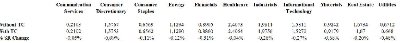
20 Table 5 – Impact of the introduction of transaction costs in SR levels (maximum SR approach and LO)
4.4. Transaction costs introduction
Even giving a more realistic interpretation, the introduction of transaction costs do not represent
the overall charges that investors need to incur to be exposed to these strategies – other brokerage
fees and additional costs such as taxes that are involved in the process, and are not being considered.
The used procedure shows that in this test, the impact of transaction costs is almost null (Table 5).
Factor investing is normally associated to transaction-intensive methods, but in this case, this is not
observed: the portfolio only readjusts its positions in a monthly frequency, leading to a total of
twelve adjustments per year – and this readjustment may even not require transactions of the
securities most of the times, what reduces substantially its impact in the obtained SR.
As explained, investors incur in other costs beyond the considered. One of these costs it is
associated with the positioning of the strategy: this strategy aims to provide an additional return
through the investing based on factors (alpha seeking) – or at least indicators that represent
implicitly these factors. Due to its specificity, it is difficult to find indexes or smart beta indexes
that replicate exactly the required positions, and this demand for flexibility turns this investment
approach in an actively managed strategy. Investors that consider this strategy as a good driver of
investment should take this into consideration, once it may increase drastically its associated costs.
4.5. Other important considerations
The obtained outputs showed us that, even with some drawbacks the design strategies can be a
21
potential benefits and risks. Being an industry-based approach – it is assessed the possibility of
industry’s segmentation through the selected ten indicators – investors should consider that the risk to be exposed to idiosyncratic risk is higher. Other important consideration is related to the extreme
outperformance of most of the industries in the out-of-sample period. Besides the small period and
the inexistence of long losses periods (where these strategies tend to suffer a lot), Europe lived a
prosperity period with GDP growth levels well above the observed in the sovereign crisis. This is
mainly sustained by the growing of the companies’ capital expenditures and ease of financing,
something not equally observed by families, being a possible explanation for the lower relative
performance of consumer staples sector. In this period, it is also underlined global appreciation in
the market for technological companies (leading to high returns levels), and the low profitability
of the communication services sector due to the change in its business models and significant
margins’ reduction, what impacted in these sectors’ performance.
5. Conclusions and Recommendations
Summing up all the conclusions and remarks above referred, we can conclude that the developed
strategies seems to provide competitive results when compared with the benchmarks for the same
period. The used procedure – which aims to provide a profitable and simple investment strategy
for the average investor – proved to work well both in in-sample and out-of-sample environments.
During the in-sample analysis, and even though risk-management strategies (risk-parity and
inverse volatility) seems to perform better in most of the industries during this period, the
indicator-based strategies also provided competitive performance. Compared with their industries proxies,
all the industries surpass its respective proxy in terms of SR and produced positive alphas, being
most of them significant at 5% significance level (7 out of 11). When compared with the market,
22
but among them, 4 industries obtained a relatively close bound. The introduction of the composite
strategy did not show positive outcomes in terms of added value when our investment decision is
based on additional factors. Similarly, this composite strategy when combined with a
risk-management strategy – the risk-averse composite approach – seems to work in terms of risk control,
but due to the weak performance of the composite strategy, its performance is not as positive as
expected. Based on these evidences, a combination between the maximum SR and a
risk-management strategy might be positive in terms of performance – reduction of the risk without
harming SR. The skewness and kurtosis levels, which are also important dimensions in investment
decisions matters, also seems to provide optimistic results both from the comparison with the
respective benchmarks and with optimal values.
The test in out-of-sample of the identified investment approaches sustained the previous
findings, where the base case approach provided higher SR in all industries when compared with
the industries proxies. However, when compared with the SR market performance, only 5 out of
10 industries surpass it. As mentioned before, the environment that surrounded the market during
these two out-of-sample years is an important dimension in the assessment of this performance.
In this tests, transaction costs do not impact much the performance of the strategies due to its
low-rebalancing frequency. However, other associated costs and charges that the investor needs to
be exposed to capture the identified premiums are an important vector not considered in this report.
The fact of being investing through sector-based approaches it is also an additional source of risk.
Even with some limitations, the results of this tests in terms of the assessment of a possible
industry segmentation through fundamental indicators seems to be positive, but investors should
consider all the remarks and risks mentioned in this report. Beyond that, investors should consider
23 Table 6 – Final output summary and industries segmented through indicators (maximum SR approach and LO)
and period size, or skew and kurt associated risks in proved tests. Other important dimension
besides the SR and skew or kurt analysis is related with the standard deviation (a risk proxy) level
that represents an important issue for investors that desire to pursue this approach in a real
investment environment. Even with these risks, the results seem to provide a good basis to develop
strategies based on these fundamental indicators or others – the considered market (European small
and medium size companies) and the sample of indicators is only a small example of the available
ones, and possibly some of them not tested here present better and more robust results. Table 6
summarizes the identified indicators and main obtained performance results for each industry.
References
• Ammann, Manuel, G. Coqueret and J. Schade. 2016. "Characteristics-based Portfolio Choice with Leverage Constraints," Journal of Banking and Finance, 70:23-37
• Ang, Andrew. 2014. Asset management: A systematic approach to factor investing. Oxford University Press.
• Basu, Sanjoy. 1977. "Investment performance of common securities in relation to their price-earnings ratios: A test of the efficient market hypothesis." The Journal of Finance,
24
• Blitz, David. 2012. “Strategic Allocations to Premiums in the Equity Market.” Journal of
Index Investing, 2(4): 42-49
• Blitz, David. 2015. “Factor Investing Revisited”. Journal of Index Investing, 6(2): 7-17 • Blitz, David. 2016. “Factor Investing with Smart Beta Indices.” The Journal of Index
Investing, 7(3): 43-48
• Brière, M. and A. Szafarz. 2015.” Factor Investing: Risk Premia vs. Diversification Benefits.” Working paper available at SSRN.
• Brière, Marie and Ariane Szafarz. 2018. "Factors and Sectors in Asset Allocation: Stronger Together?," Working Papers CEB 18-016, ULB - Universite Libre de Bruxelles
• Carhart, Mark. 1997. "On persistence in mutual fund performance." The Journal of
Finance, 52(1): 57-82
• Cazalet, Zélia and T. Roncalli. 2014. “Facts and Fantasies About Factor Investing.” Working paper available at SSRN
• Chen, N.F., R. Roll and S.A. Ross. 1986. “Economic forces and the stock market.” Journal
of Business, 59: 383–403
• Fama, Eugene and Kenneth R. French, 2015. "Incremental variables and the investment opportunity set," Journal of Financial Economics, 117(3): 470-488
• Fama, Eugene F., and Kenneth R. French. 1992. “The cross-section of expected stock returns.” The Journal of Finance, 47: 427–465
• Fama, Eugene F., and Kenneth R. French. 1996. “Multifactor Explanations of Asset Pricing Anomalies.” The Journal of Finance, 51(1): 55–84
25
• Haugen, Robert A., and Nardin L. Baker. 1996. “Commonality in the determinants of expected stock returns.” Journal of Financial Economics, 41: 401-439
• Hsu, Jasin and Vitali Kalesnik. 2014. “Finding Smart Beta in the Factor Zoo.” Research Affiliates
• Hsu, Jason, V. Kalesnik and V. Viswanathan. 2015. “A framework for assessing factors and implementing smart betas strategies.” The Journal of Index Investing, 6(1): 89-97 • Huij, Joop, S. Lansdorp, David Blitz and Pim van Vliet. 2014. “Factor Investing:
Long-Only versus Long-Short”. Working paper available at SSRN
• Jegadeesh, Narasimhan, and Sheridan Titman. 1993. "Returns to buying winners and selling losers: Implications for stock market efficiency." The Journal of Finance, 48: 65-91
• Kacperczyk, Marcin T., C. Sialm and Lu Zheng. 2005. “On the Industry Concentration of Actively Managed Equity Mutual Funds.” The Journal of Finance, 60(4): 1983-2011 • Koedijk, Kees G., Alfred M.H. Slager and Philip A. Stork. 2016. “Investing in Systematic
Factor Premiums.” The Journal of Portfolio Management, 22(2): 193–234
• Lewellen, Jonathan, 2014, “The Cross Section of Expected Stock Returns.” Forthcoming
in Critical Finance Review, 4: 1–44
• McLean, R. David, and Jeffrey Pontiff. 2016. “Does Academic Research Destroy Stock Return Predictability?” The Journal of Finance, 71: 5-32.
• Moskowitz, Tobias J. and Mark Grinblatt. 2016. “Do Industries Explain Momentum?” The
Journal of Finance, 54(4): 1249-1290
26 Appendix A – Industries’ metrics considered for test issues
Appendix B – Indicators that provided the highest SR level for each industry (maximum SR approach)
1 Appendix C – List of companies downloaded per industry (Name and Ticker)
Crossed companies were not considered for test issues
Additional Appendix
This appendix was constructed for better understanding purposes. Due to size issues, the provided
graphs that replicate some outputs of the model will only be provided for the industrials industry.
Industrials
Safran SA (SAF FP Equity); Airbus SE (AIR FP Equity); Schneider Electric SE (SU FP Equity); Vinci SA (DG FP Equity); Kone Oyj-B (KNEBV FH Equity); Teleperformance (TEP FP Equity); Edenred (EDEN FP Equity); Prysmian Spa (PRY IM Equity); Gea Group AG (G1A GY Equity); Rheinmetall AG (RHM GY Equity); Ryanair Holdings PLC (RYA ID Equity); Deutsche Lufthansa-REG (LHA GY Equity); Wartsila OYJ ABP (WRT1V FH Equity); Air France-KLM (AF FP Equity); Siemens AG-REG (SIE GY Equity); Kingspan Group PLC (KSP ID Equity); Osram Licht AG (OSR GY Equity); Randstad NV (RAND NA Equity); Wolters Kluwer (WKL NA Equity); Brenntag AG (BNR GY Equity); Rexel SA (RXL FP Equity); Deutsche Post AG-REG (DPW GY Equity); Cnh Industrial NV (CNHI IM Equity); Bouygues SA (EN FP Equity); Signify NV (LIGHT NA Equity); Konecranes OYJ (KCR FH Equity); Leonardo SPA (LDO IM Equity); Boskalis Westminster (BOKA NA Equity); Elis SA (ELIS FP Equity); ACS Actividades Cons Y Serv (ACS SQ Equity); Alstom (ALO FP Equity); Andritz AG (ANDR AV Equity); Bollore (BOL FP Equity); Imcd NV (IMCD NA Equity); Hochtief AG (HOT GY Equity); Dassault Aviation SA (AM FP Equity); Thales SA (HO FP Equity); Mtu Aero Engines AG (MTX GY Equity); Compagnie De Saint Gobain (SGO FP Equity); Kion Group AG (KGX GY Equity); Metso OYJ (METSO FH Equity); ADP (ADP FP Equity); Spie SA (SPIE FP Equity); Aalberts Industries NV (AALB NA Equity); Legrand SA (LR FP Equity); Bureau Veritas SA (BVI FP Equity); Ferrovial SA (FER SQ Equity); Valmet OYJ (VALMT FH Equity); Aena Sme SA (AENA SQ Equity); Atlantia SPA (ATL IM Equity); Getlink (GET FP Equity); Eiffage (FGR FP Equity); Societe BIC SA (BB FP Equity); Siemens Gamesa Renewable ENE (SGRE SQ Equity); Fraport AG Frankfurt Airport (FRA GY Equity); MAN SE (MAN GY Equity).
Materials
Lin (LIN GY Equity); CRH PLC (CRH ID Equity); Koninklijke DSM NV (DSM NA Equity); Basf SE (BAS GY Equity); Umicore (UMI BB Equity); Arcelormittal (MT NA Equity); Akzo Nobel (AKZA NA Equity); Air Liquide SA (AI FP Equity); SMURFIT Kappa Group PLC (SKG ID Equity); Arkema (AKE FP Equity); Solvay SA (SOLB BB Equity); Symrise AG (SY1 GY Equity); Covestro AG (1COV GY Equity); Aurubis AG (NDA GY Equity); Wacker Chemie AG (WCH GY Equity); Upm-Kymmene OYJ (UPM FH Equity); Huhtamaki OYJ (HUH1V FH Equity); K+S AG-REG (SDF GY Equity); Thyssenkrupp AG (TKA GY Equity); Fuchs Petrolub SE -PREF (FPE3 GY Equity); Stora Enso OYJ-R SHS (STERV FH Equity); Lanxess AG (LXS GY Equity); Evonik Industries AG (EVK GY Equity); Imerys SA (NK FP Equity); Heidelbergcement AG (HEI GY Equity); Wienerberger AG (WIE AV Equity); Voestalpine AG (VOE AV Equity).
Informational Technologies
Asml Holding NV (ASML NA Equity); Infineon Technologies AG (IFX GY Equity); Wirecard AG (WDI GY Equity); SAP SE (SAP GY Equity); Stmicroelectronics NV (STM IM Equity); Dassault Systemes SA (DSY FP Equity); Capgemini SE (CAP FP Equity); ATOS SE (ATO FP Equity); Amadeus IT Group SA (AMS SQ Equity); NOKIA OYJ (NOKIA FH Equity); Adyen NV (ADYEN NA Equity); Siltronic AG (WAF GY Equity); ASM International NV (ASM NA Equity); Software AG (SOW GY Equity); Nemetschek SE (NEM GY Equity); Ingenico Group (ING FP Equity); Bechtle AG (BC8 GY Equity); Alten SA (ATE FP Equity); Altran Technologies SA (ALT FP Equity); Gemalto (GTO NA Equity); Sopra Steria Group (SOP FP Equity).
Energy
Total SA (FP FP Equity); Galp Energia SGPS SA (GALP PL Equity); Saipem SPA (SPM IM Equity); Tenaris SA (TEN IM Equity); Snam SPA (SRG IM Equity); OMV AG (OMV AV Equity); SBM Offshore NV (SBMO NA Equity); Neste OYJ (NESTE FH Equity); Vopak (VPK NA Equity); Enagas SA (ENG SQ Equity); ENI SPA (ENI IM Equity); Technipfmc PLC (FTI FP Equity); Repsol SA (REP SQ Equity).
Healthcare
Siemens Healthineers AG (SHL GY Equity); Biomerieux (BIM FP Equity); Galapagos NV (GLPG NA Equity); Orion OYJ-CLASS B (ORNBV FH Equity); Recordati SPA (REC IM Equity); Koninklijke Philips NV (PHIA NA Equity); Carl Zeiss Meditec AG - BR (AFX GY Equity); Morphosys AG (MOR GY Equity); UCB SA (UCB BB Equity); Evotec AG (EVT GY Equity); Merck KGAA (MRK GY Equity); Fresenius SE & CO KGAA (FRE GY Equity); Diasorin SPA (DIA IM Equity); Sanofi (SAN FP Equity); Fresenius Medical Care AG & (FME GY Equity); Eurofins Scientific (ERF FP Equity); Essilorluxottica (EL FP Equity); Sartorius Stedim Biotech (DIM FP Equity); Sartorius AG-Vorzug (SRT3 GY Equity); Argenx SE (ARGX BB Equity); Bayer AG-REG (BAYN GY Equity); Gerresheimer AG (GXI GY Equity); Orpea (ORP FP Equity); IPSEN (IPN FP Equity); Grifols SA (GRF SQ Equity); Qiagen N.V. (QIA GY Equity).
2 Communication Services
Axel Springer SE (SPR GY Equity); Proximus (PROX BB Equity); Lagardere SCA (MMB FP Equity); Freenet AG (FNTN GY Equity); Rtl Group (RRTL GY Equity); Deutsche Telekom AG-REG (DTE GY Equity); Telefonica SA (TEF SQ Equity); Telenet Group Holding NV (TNET BB Equity); Telecom Italia SPA (TIT IM Equity); Orange (ORA FP Equity); Publicis Groupe (PUB FP Equity); Prosiebensat.1 Media SE (PSM GY Equity); SES (SESG FP Equity); Jcdecaux SA (DEC FP Equity); Vivendi (VIV FP Equity); Eutelsat Communications (ETL FP Equity); Cellnex Telecom SA (CLNX SQ Equity); Elisa OYJ (ELISA FH Equity); 1&1 Drillisch AG (DRI GY Equity); Iliad SA (ILD FP Equity); United Internet AG-REG Share (UTDI GY Equity); SCOUT24 AG (G24 GY Equity); Telefonica Deutschland Holdi (O2D GY Equity); Koninklijke KPN NV (KPN NA Equity); Ubisoft Entertainment (UBI FP Equity).
Consumer Discretionary
SEB SA (SK FP Equity); HELLA GMBH & CO KGAA (HLE GY Equity); Industria De Diseno Textil (ITX SQ Equity); Moncler SPA (MONC IM Equity); Michelin (CGDE) (ML FP Equity); Plastic Omnium (POM FP Equity); Puma SE (PUM GY Equity); Lvmh Moet Hennessy Louis Vui (MC FP Equity); Christian Dior SE (CDI FP Equity); Porsche Automobil HLDG-PRF (PAH3 GY Equity); Accor SA (AC FP Equity); Sodexo SA (SW FP Equity); Peugeot SA (UG FP Equity); Renault SA (RNO FP Equity); Nokian Renkaat OYJ (NRE1V FH Equity); Adidas AG (ADS GY Equity); Luxottica Group SPA (LUX IM Equity); Zalando SE (ZAL GY Equity); Delivery Hero SE (DHER GY Equity); Kering (KER FP Equity); Volkswagen AG-PREF (VOW3 GY Equity); Valeo SA (FR FP Equity); Amer Sports OYJ (AMEAS FH Equity); FIAT Chrysler Automobiles NV (FCA IM Equity); Hugo Boss AG -ORD (BOSS GY Equity); Hermes International (RMS FP Equity); Ferrari NV (RACE IM Equity); Continental AG (CON GY Equity); Faurecia (EO FP Equity); Paddy Power Betfair PLC (PPB ID Equity); Daimler AG-Registered Shares (DAI GY Equity); Bayerische Motoren Werke AG (BMW GY Equity); Pirelli & C SPA (PIRC IM Equity).
Financials
Erste Group Bank AG (EBS AV Equity); Deutsche Boerse AG (DB1 GY Equity); Deutsche Bank AG-Registered (DBK GY Equity); Bolsas Y Mercados Espanoles (BME SQ Equity); ABN Amro Group NV-CVA (ABN NA Equity); UBI Banca SPA (UBI IM Equity); Banco Comercial Portugues-R (BCP PL Equity); Natixis (KN FP Equity); Unicredit SPA (UCG IM Equity); Caixabank SA (CABK SQ Equity); Banco BPM SPA (BAMI IM Equity); Finecobank SPA (FBK IM Equity); Bankinter SA (BKT SQ Equity); Intesa Sanpaolo (ISP IM Equity); Exor NV (EXO IM Equity); Amundi SA (AMUN FP Equity); Sampo OYJ-A SHS (SAMPO FH Equity); Eurazeo SE (RF FP Equity); Poste Italiane SPA (PST IM Equity); Ackermans & Van Haaren (ACKB BB Equity); Banco Santander SA (SAN SQ Equity); Bank Of Ireland Group PLC (BIRG ID Equity); Societe Generale SA (GLE FP Equity); Muenchener Rueckver AG-REG (MUV2 GY Equity); Mapfre SA (MAP SQ Equity); ASR Nederland NV (ASRNL NA Equity); Commerzbank AG (CBK GY Equity); Credit Agricole SA (ACA FP Equity); Bankia SA (BKIA SQ Equity); Euronext NV (ENX FP Equity); Grenke AG (GLJ GY Equity); Assicurazioni Generali (G IM Equity); Aareal Bank AG (ARL GY Equity); AIB Group PLC (AIBG ID Equity); CNP Assurances (CNP FP Equity); Groupe Bruxelles Lambert SA (GBLB BB Equity); Banco Bilbao Vizcaya Argenta (BBVA SQ Equity); Raiffeisen Bank International (RBI AV Equity); KBC Group NV (KBC BB Equity); Sofina (SOF BB Equity); NN Group NV (NN NA Equity); ING Groep NV (INGA NA Equity); Mediobanca SPA (MB IM Equity); Wendel (MF FP Equity); AXA SA (CS FP Equity); BNP Paribas (BNP FP Equity); Banco De Sabadell SA (SAB SQ Equity); Aegon NV (AGN NA Equity); Hannover Rueck SE (HNR1 GY Equity); Allianz SE-REG (ALV GY Equity); Scor SE (SCR FP Equity); Ageas (AGS BB Equity).
Consumer Staples
Kerry Group PLC-A (KYG ID Equity); Viscofan SA (VIS SQ Equity); Anheuser-Busch Inbev SA/NV (ABI BB Equity); Beiersdorf AG (BEI GY Equity); Henkel AG & CO Kgaa Vorzug (HEN3 GY Equity); Danone (BN FP Equity); Davide Campari-Milano SPA (CPR IM Equity); Metro AG (B4B GY Equity); Colruyt SA (COLR BB Equity); Unilever NV-CVA (UNA NA Equity); Koninklijke Ahold Delhaize N (AD NA Equity); Kesko OYJ-B SHS (KESKOB FH Equity); Carrefour SA (CA FP Equity); Glanbia PLC (GLB ID Equity); Heineken NV (HEIA NA Equity); Heineken Holding NV (HEIO NA Equity); Jeronimo Martins (JMT PL Equity); Remy Cointreau (RCO FP Equity); Pernod Ricard SA (RI FP Equity); L'OREAL (OR FP Equity).
Real estate
Covivio (COV FP Equity); Aroundtown SA (AT1 GY Equity); Gecina SA (GFC FP Equity); Vonovia SE (VNA GY Equity); Merlin Properties Socimi SA (MRL SQ Equity); LEG Immobilien AG (LEG GY Equity); Klepierre (LI FP Equity); Inmobiliaria Colonial Socimi (COL SQ Equity); TAG Immobilien AG (TEG GY Equity); Cofinimmo (COFB BB Equity); UNIBAIL-Rodamco-Westfield (URW NA Equity); ICADE (ICAD FP Equity); Deutsche Wohnen SE (DWNI GY Equity).
Utilities
Iberdrola SA (IBE SQ Equity); E.ON SE (EOAN GY Equity); EDF (EDF FP Equity); ENEL SPA (ENEL IM Equity); Veolia Environnement (VIE FP Equity); Naturgy Energy Group SA (NTGY SQ Equity); Engie (ENGI FP Equity); RWE AG (RWE GY Equity); Suez (SEV FP Equity); Endesa SA (ELE SQ Equity); Uniper SE (UN01 GY Equity); RED Electrica Corporacion SA (REE SQ Equity); Rubis (RUI FP Equity); Terna SPA (TRN IM Equity); EDP-Energias De Portugal SA (EDP PL Equity); Italgas SPA (IG IM Equity); Fortum OYJ (FORTUM FH Equity); A2A SPA (A2A IM Equity); Innogy SE (IGY GY Equity).
3 Appendix D – Summary correlation table (Industrials Industry and LO), in-sample analysis
Appendix E – Annual average return, Annual standard deviation and SR summary table for each indicator (Industrials Industry and LO), in-sample analysis
Appendix F – SR Summary Table of each traditional strategy tested (Industrials Industry and LO), in-sample analysis
Appendix G – Traditional strategies summary output (Industrials Industry and LO), in-sample analysis It summarizes the overall output for each industry, based on the different defined approaches. Negative alphas are marked in red
and non-significant ones (at 5% confidence level) are highlighted. Industry and market proxies’ performance are also presented here.
4 Appendix H – Maximum Annual Average Return indicator summary output (Industrials Industry and LO), in-sample analysis
Appendix I – Minimum Annual Average Return indicator summary output (Industrials Industry and LO), in-sample analysis
5 Appendix J – Maximum SR indicator summary output (Industrials Industry and LO), in-sample analysis
Appendix K – Composite Strategy summary output (Industrials Industry and LO), in-sample analysis
6 Appendix M – Maximum Annual Average Return indicator summary output (Industrials Industry and LO), out-of-sample analysis
Appendix N – Minimum Annual Average Return indicator summary output (Industrials Industry and LO), out-of-sample analysis
7 Appendix P – Composite Strategy summary output (Industrials Industry and LO), out-of-sample analysis