ISSN 0101-7438
THE STRATEGY OF EMPIRICAL RESEARCH AND OPTIMIZATION PROCESS
L.E. Brossard Perez* L.A.B. Cortez+† J. Mesa* G. Bezzon+
E.Olivares Gómez++
*
Universidad de Oriente
Departamento de Ingeniería Química Santiago de Cuba – Cuba
Email: [email protected]
+
Universidade Estadual de Campinas
Núcleo Interdisciplinar de Planejamento Energético (NIPE) Campinas, SP – Brazil
Email: [email protected]
++
Universidade Estadual de Campinas
Faculdade de Engenharia Agrícola-FEAGRI Campinas, SP – Brazil
Email: [email protected]
† To whom correspondence should be addressed
Abstract
Empirical modeling is considered from the perspectives of a general scheme for the Strategy of Empirical Research and Optimization Process (SEROP). This approach intends to facilitate the understanding of the necessary steps to arrive to mathematical models able to appropriately describe the behavior of a group of controllable independent variables related to a certain response. Aspects connected with definition of the problem, variable’s identification and optimization stages are discussed. As an example of SEROP application, it is presented the empirical modeling of the basic extraction of alginic acid from brown algae.
1. Introduction
The study of a technical or scientific situation, usually presents two different and, in many ways, complementary points of view. These are:
a) a generalized phenomenological description and;
b) a limited empirical modelling.
Human knowledge is continuously fed by both approaches and there are countless examples of interactions between them. When the problem is to find a proper description of a process in a short time, at low costs and with the necessary accuracy, the dilemma emerges. Although theoretical models are to be preferred, they are unfortunately not available for every new practical situation. In these cases, empirical models may be used, knowing that their results are limited to the experimental region in which they were obtained. This drawback can be of no importance if what is sought is the behavior of a particular process in a set of particular conditions. However, empirical models building has also its own rules, that should be followed in order to arrive at reliable information.
Author’s own experience in the field of empirical modelling is presented in this paper as a modest contribution for better planned and interpreted experimental work.
The paper is divided in three parts:
1. the search for the optimum;
2. practical considerations;
3. illustrative example.
2. The search for the optimum
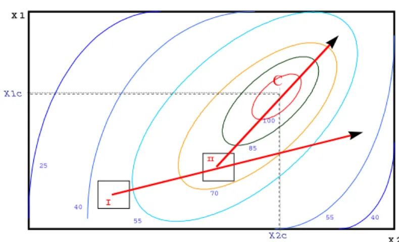
In a well defined problem, where responses are correctly selected and where a screening process for the reduction of the identified independent variables has been applied, a search for the optimum can be conducted. The search is limited to an experimental region in which only one stationary point should be found.
Figure 1 shows the hypothetical boundaries of an experimental region where responses are plotted as contour lines, considered factors are X1 and X2. Points I and II represented the zones where initial exploring experimental designs are carried out and Point C stands for the optimum (a maximum in this example).
X 1
100
85
70
55 55
40
40 25
X 2c X 1c
X 2 I
II
C
Figure 1 – Boundaries of a system with an optimum.
The procedure is repeated until curvature effects begin to be noticeable. In this point of the search, it is advisable to establish the trajectory for best performance by means of the steepest ascent method.
At the end of this last step, a new two level factorial design is conducted. The resulting model will show a big curvature effect, indicating that a second order design will describe the exact position of the stationary point. The obtained second order model is best analyzed through its response surface.
The search for the optimum is in no way a simple trial and error process and needs careful attention in every step. At this point it should be remembered that not all empirical studies have to end with an optimization process. This case takes place when the only objective is to describe conditions under which a certain process operates and there is no intention or possibility to change it.
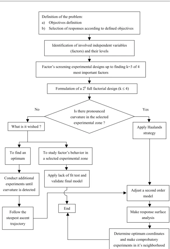
In order to organize the different stages in the search for the optimum and also to include the simpler situation just mentioned above, a general scheme for the strategy of empirical research and optimization process (SEROP) is presented in Figure 2.
3. Practical considerations about steps of SEROP
Problem definition: To define the objective of an investigation, it is necessary to conduct an information searching process that will allow answering the following questions:
a) Which will be the responses to be studied and which is their hierarchy order?
It is important to establish a hierarchical order when more than one answer is selected, because they will be affected by the same factors, making it frequently impossible to find a combination of the given factors that optimizes all answers at the same time.
b) Which are the independent factors that may affect the answers?
Definition of the problem: a) Objectives definition
b) Selection of responses according to defined objectives
Identification of involved independent variables (factors) and their levels
Factor’s screening experimental designs up to finding k=3 of 4 most important factors
Formulation of a 2k full factorial design (kd 4)
Is there pronounced curvature in the selected
experimental zone ?
What is it wished ? Apply Haalands
strategy
To find an optimum
To study factor’s behavior in a selected experimental zone
Follow the steepest ascent
trajectory
Apply lack of fit test and validate final model
Adjust a second order model
Make response surface analysis End
Determine optimum coordinates and make comprobatory experiments in it’s neighborhood Conduct additional
experiments until curvature is detected
Yes No
3.1 Selection of the experimental zone under study
The space occupied by the experiment will be determined by the separation that exists between the higher and lower levels of each factor.
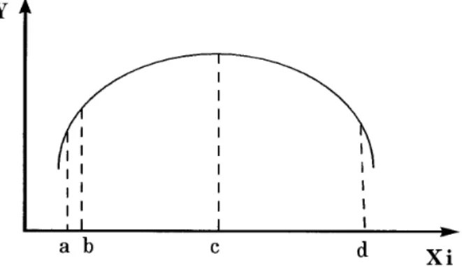
1. if the levels are chosen too closely, it is possible that the response variation (Y) is not observed in the experiment or may have the order of magnitude of the stochastic fluctuations, and therefore the model will be Y = constant. (Figure 3, a d Xid b)
2. if the levels are chosen too for apart, two mistakes may be made. (Figure 3, a d Xid d)
x The points “a” and “d” may be found on both sides of a maximum or a minimum and the difference between the Y value results may be impossible to be observed.
x The experimental errors made at different points of the region being significantly distinct, indicating in this case a lack of variance homogeneity and therefore the utilized parametric tests, for example t and F, would not be powerful enough, because they are based on the assumption that variance homogeneity exists, among other conditions.
The interval (Figure 3, a d Xi d c) gives more reliable results, a since it contains relevant changes in the response. Naturally, before conducting the experiments, these situations are unknown, therefore the initial selection of values of the operating variables will be affected by Guerra Debén & Sevilla (1988):
a) the historical knowledge of the system under study; b) the available theory;
c) the existence of exploratory experiments; d) the luck factor.
Figure 3 – Behavior of response Y when the level of the Xi factor is varied
3.2 The screening of independent variables (Sutton, 1997; Box et al., 1993; and Barros Netoet al., 1995)
If a factor of strong influence over the response, is not controlled, it won’t be possible to obtain reliable results due to the large fluctuations that are to be observed in the response, and what is even worse, the noted behavior can be wrongly attributed to some of the controlled factors. It can also be the case that it is not possible to introduce changes in a known important factor. In such cases, the wisest thing to do is to control it at a definite favorable level. Thus, the obtained results are said to be conditioned or restricted by the factor.
3.3 Formulation of a 2k full factorial design
When screening work is finished, the number of independent variables should be around 4 or less. It is possible, however, to count with a fractioned design having also a maximum of 16 experiments in its planning. These numbers are not rigid limits and specific conditions will have the last word. Box et al. (1993) as well as Barros Neto et al. (1995) are excellent treatises in this respect.
3.4 Curvature check
When a supposed linear model, contains interaction’s coefficients as big as or even bigger than individual factor’s coefficients, the corresponding response surface will show curvature. There are cases where curvature, although present, is rather slight and the obtained model shows no lack of fit. However, if curvature is pronounced, linear models are not able to represent experimental behavior and need to be replaced by second order models.
Curvature can also be evaluated quantitatively by means of central points replicates. This will be shown in the illustrative example.
3.5 Establishing the trajectory for best performance
If the main objective of the research is to find either a maximum or a minimum for the studied response, several strategies are available. One, or perhaps the most known method, is the method of steepest ascent (Box et al., 1993), which makes use of a few exploratory points conducted according to a stepwise change in the levels of the involved factors. This change is determined by a reference factor, that usually is the one with the highest coefficient in the linear model.
In this way, an experimental trajectory is followed until a change is noted in the direction of response’s increase. This point of rupture gives the necessary information about both sides of the noted change (possible stationary point) and allows a proper factor levels selection for a new two level factorial design. The resulting linear model will show a great curvature effect. This last obtained linear model is used at the nucleus of a second order design, which requires additional experimental points to fully describe the optimum zone.
3.6 Second order design (Montgomery, 1991) Two of the most used second order designs are:
x Central composite orthogonal designs;
x Central composite rotational designs.
Both types of designs are carried out sequentially. This means that the information obtained from a full or fractional design is used in the data processing after adding new experiments according to the characteristics of each design.
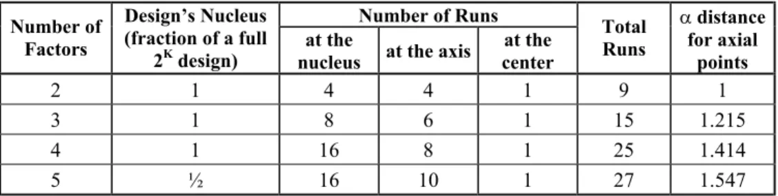
3.6.1 Central composite orthogonal designs (CCOD) These designs are distinguished by (see Table 1):
x having a nucleus made out of a full factorial design or a fraction of it;
x two extra runs for each factor, located at a coded D distance from the center of the experimental region. These are called axial points as they are at (+) D and (–) D distance from the zero point on the factors axes.
x one or more runs at the center of the design.
Table 1– Structures of Central Composed Orthogonal Designs Number of Runs
Number of Factors
Design’s Nucleus (fraction of a full
2K design)
at the
nucleus at the axis
at the center
Total Runs
D distance for axial
points
2 1 4 4 1 9 1
3 1 8 6 1 15 1.215
4 1 16 8 1 25 1.414
5 ½ 16 10 1 27 1.547
Second order CCOD have higher precision when:
x optimum finds itself in the close neighborhood of experimental zone’s center. This is perfectly possible if an adequate optimization strategy (i.e. – steepest ascent method) has been followed or the investigators own experience indicates this is so;
x there are no time changes in experimental responses between first experiments (at the nucleus) and additional experiments (center and axis);
x variance is approximately the same for all experimental points located at equal distance from the center of the design.
3.6.2 Central composite rotational designs (CCRD)
Table 2 – Structure of CCRD
Number of Runs Number of
Factors
Design’s nucleus (fraction’s of a
full 2K design) nucleusat the at the axis centerat the
Total Runs
D distance for axial
points
2 1 4 4 5 13 1.414
3 1 8 6 6 20 1.682
4 1 16 8 7 31 2.000
5 1/2 16 10 6 32 2.000
4. Example of SEROP
Alkaline extraction of alginic acid from brown algae (Mesa Pérez et al., 1998)
Problem Definition: Brown algae, previously crushed and acidified with HCl solution, contains alginic acid that is intended to be extracted in the form of its sodium salt.
The final product, once purified, has many industrial applications based on the viscosity of its aqueous solutions. The research objective is to test an extraction method based on the reaction of a solution of sodium carbonate with alginic acid inside acid treated algae residues. The operation is batch wise conducted at room temperature (26ºC) under agitation. To evaluate if the objective is achieved, two responses are to be followed:
x yield of sodium alginate;
x viscosity of 1% aqueous solution of sodium alginate.
To be brief, only viscosity will be treated here.
4.1 Identification of factors
Initial acid treated algae as well as sodium carbonate solutions came from the same stock. All experiments were performed in the same reactor with the same reaction time and same operators.
A constant agitation speed was adopted throughout all experimental work. Under these conditions no screening was considered necessary and the following factors were identified together with their levels (see Table 3). Of course, this is a simplified situation. Screening work is almost always necessary when beginning to study a new problem.
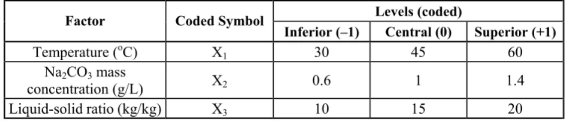
Table 3 – Alkaline extraction of acid treated brown algae (identified factors, symbols, and levels)
Levels (coded)
Factor Coded Symbol
Inferior (–1) Central (0) Superior (+1)
Temperature (oC) X1 30 45 60
Na2CO3 mass
concentration (g/L) X2 0.6 1 1.4
Liquid-solid ratio (kg/kg) X3 10 15 20
4.2 Formulation of a 2K full factorial design
As K=3, a 23 = 8 experiments full factorial design is chosen.
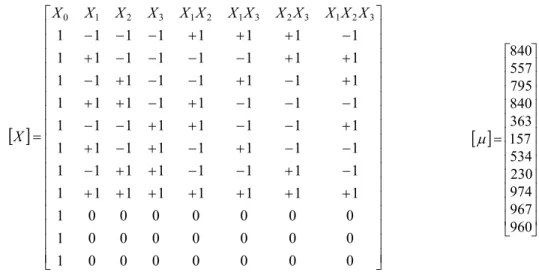
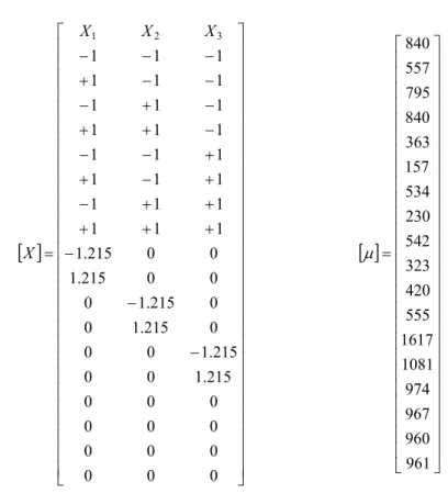
Independent variable matrix (X matrix) (includes experiment matrix), as well as response matrix (P matrix) are shown below:
> @
» » » » » » » » » » » » » » » » » ¼ º « « « « « « « « « « « « « « « « « ¬ ª 0 0 0 0 0 0 0 1 0 0 0 0 0 0 0 1 0 0 0 0 0 0 0 1 1 1 1 1 1 1 1 1 1 1 1 1 1 1 1 1 1 1 1 1 1 1 1 1 1 1 1 1 1 1 1 1 1 1 1 1 1 1 1 1 1 1 1 1 1 1 1 1 1 1 1 1 1 1 1 1 1 1 1 1 1 1 1 1 3 2 1 3 2 3 1 2 1 3 2 10 X X X X X X X X X X X X
X
X
> @
» » » » » » » » » » » » ¼ º « « « « « « « « « « « « ¬ ª 960 967 974 230 534 157 363 840 795 557 840 P
Following a well known procedure (Montgomery, 1991), first order model is obtained. The corresponding analysis of variance is shown in Table 4.
Table 4 – ANOVA for first order model
Variation source SS df MSS F test p-value
X1 69938 1 69938 1427 0.0007
X2 29040.5 1 29040.5 593 0.0017
X3 381938 1 381938 7795 0.0001
X1 X2 6612.5 1 6612.5 135 0.0073
X1 X3 9248 1 9248 189 0.0053
X1 X2 X3 22684.5 1 22684.5 463 0.0022
Lack of fit 398745.4 2 199372.7 4069 0.0002
Pure error 98 2 49
Total (Corr) 918304.9 10
R2 = 0.57
After testing for coefficients significance at D = 0.05 level, the coded final model is:
... (4.2.1) 3 2 1 3 1 2 1 3 2
1 60 218 29 34 53
93
656 X X X X X X X X X X
P
of individual factors. An analysis of variance, in this case, will show that the regression sum of squares is quite smaller than the total sum of squares and that there exists a large and, therefore, significative lack of fit in the model.
Of course, a curvature check is always possible. Thus,
Curvature Effect =
y2y1rtD,v Sexp... (4.2.2)1
y = average of the n1 experimental responses of the design (here n1 = 8 and y1= 539.5)
2
y = average of the n2 center points (here n2 = 3 and y2= 967)
t = student statistic (two tailed’s test)
D = significance level = 0.05
v = degrees of freedom of Sexp (here v = 2)
exp
S = standard deviation of pure error (here S = 7), and so
Curvature Effect = (967 – 539.5) r t (0.05, 2) (7) = 427.5 r 4.3 . (7) = 427 r 30
This result shows that responses at the center points are well higher than those belonging to the base design points and constitute a quantitative proof of curvature.
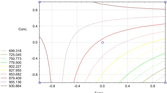
A closer look to the obtained model shows that factor X3 (liquid-solid ratio) should work at the lowest level in order to obtain greater viscosities. Figure 4, shows response surface for a fixed X3 = –1 level. It is clearly seen, that viscosity reaches a so called saddle point, that can’t be described completely by the so far obtained model.
699.318 725.045 750.773 776.500 802.227 827.955 853.682 879.409 905.136 930.864
Temp. Conc.
-0.8 -0.4 0.0 0.4 0.8
-0.8 -0.4 0.0 0.4 0.8
Figure 4 – Response Surface for Viscosity Behavior at X3 = –1 (First order model)
307.864 342.136 376.409 410.682 444.955 479.227 513.500 547.773 582.045 616.318
Temp. Conc.
-0.8 -0.4 0.0 0.4 0.8
-0.8 -0.4 0.0 0.4 0.8
Figure 5 – Response Surface for Viscosity Behavior at X3 = +1 (First order model)
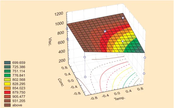
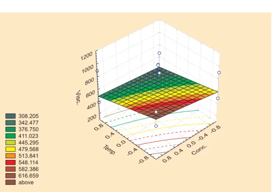
A tridimensional picture of both cases is given in Figure 6 and 7. In this particular case, a lowering of the liquid-solid ratio (X3) should have it’s limits because otherwise power increase due to stirring could be too high. Also, a point may be attained where very little or no liquid exits. This is, of course, a hypothetical situation, but helps to make a reasonable appreciation of how to change factor’s levels.
699.659 725.386 751.114 776.841 802.568 828.295 854.023 879.750 905.477 931.205 above
1200
1000
800
600
400
200
0.8
0.4
0.0
-0.4
-0.8
V
isc.
Conc.
Temp.
-0.8 -0.4
0.0 0.4
0.8
308.205 342.477 376.750 411.023 445.295 479.568 513.841 548.114 582.386 616.659 above
0.8
0.4
0.0
-0.4
-0.8 Temp.
1200
1000
800
600
400
200 V isc.
-0.8
-0.4 0.0 0.4 0.8
Conc.
Figure 7 – Tridimensional picture of first order model for X3 = +1
According to the SEROP scheme, it is recommended now to adjust a second order model due to the fact that the lineal model does not describe adequately viscosity behavior.
4.3 Adjustment of a second order model (Montgomery, 1991)
As there were evidences of a maximum in the vicinity of the initially studied experimental region, a CCOD was tried, making use of former 23 full factorial as nucleus of the new design and performing 6 new experiments for the axial points (D= 1.215). An additional center point is also added in order to improve precision, although three of them are already done. The corresponding experimental matrix as well as the response matrix are:
2 exp
> @
> @
» » » » » » » » » » » » » » » » » » » » » » » » » » ¼ º « « « « « « « « « « « « « « « « « « « « « « « « « « ¬ ª » » » » » » » » » » » » » » » » » » » » » » » » » » » » ¼ º « « « « « « « « « « « « « « « « « « « « « « « « « « « « ¬ ª 961 960 967 974 1081 1617 555 420 323 542 230 534 157 363 840 795 557 840 0 0 0 0 0 0 0 0 0 0 0 0 215 . 1 0 0 215 . 1 0 0 0 215 . 1 0 0 215 . 1 0 0 0 215 . 1 0 0 215 . 1 1 1 1 1 1 1 1 1 1 1 1 1 1 1 1 1 1 1 1 1 1 1 1 1 3 2 1 P X X X XAfter obtaining a second order model, ANOVA is conducted (Table 5).
Table 5 – ANOVA for second order model
Variation
source SS df MSS F test p-value
X1 93894 1 93894 2253 0.0000
X2 38105 1 38105 915 0.0001
X3 525577 1 525577 12614 0.0000
X1 X2 6613 1 6613 159 0.0011
X1 X3 9248 1 9248 222 0.0007
X1 X2 X3 22685 1 22685 544 0.0002
2 1
X 677441 1 677441 16259 0.0006
2 2
X 544965 1 544965 13079 0.0000
2 3
X 349098 1 349098 8378 0.0000
Lack of fit 87 5 17 0.42 0.8164
Pure error 125 3 42
Total (Corr) 2259454 17
The final coded model, after significance tests for the coefficients and a lack of fit test for the model are done, is:
2 3 2
2 2
1 3
2 1 3 1 2 1 3 2
1 59 219 29 34 53 361 324 259
93
966 X X X X X X X X X X X X X
P
(4.3.1)
4.4 Analysis of response’s surfaces
If in former model X3 is fixed at –1 level, following model is obtained:
Model 1: (X3 = –1)
... (4.4.1) 2
2 2
1 2
1 2
1 59 782 361 324
59
1444 X X X X X X
P
357.286 466.545 575.804 685.063 794.321 903.580 1012.839 1122.097 1231.356 1340.615 above
1200
800
400 1600
V
isc.
-1.2 -0.8
-0.4 0.0
0.4 0.8
1.2
Temp.
Conc.
-1.2 -0.8 -0.4 0.0 0.4 0.8 1.2
Figure 8 – Response Surface for Viscosity Behavior (Second Order model for X3 = –1)
Now, holding X3 at +1 level, a new model can be shown:
Model 2: When X3 = +1
... (4.4.2) 2
2 2
1 2
1 2
1 59 24 361 324
1267
1006 X X X X X X
92.471 184.942 277.414 369.885 462.356 554.827 647.298 739.770 832.241 924.712 above
1200
800
400 1600
V
isc.
-1.2 -0.8
-0.4 0.0
0.4 0.8 1.2
Temp. -1.2
-0.8 -0.4 0.0 0.4 0.8 1.2
Conc.
Figure 9 – Response Surface for Viscosity Behavior (Second Order model for X3 = +1)
Response’s surfaces for both models are presented in Figure 7.
Both maximum points are conditioned by the values assigned to X3 and as expected are quite different.
4.5 Determination of the optimum point
In order to obtain the coordinates of the stationary point i
wF wP
= 0 (i being 1 and 2) are determined
for each model and from the solution of both equation systems, the conditional maximum coordinates are obtained. Thus, for model 1 (X3 = –1), maximum viscosity is reached at:
X1: Temperature = 44oC
X2: Na2CO3 mass concentration = 1.036 g/L X3: Liquid-solid mass ratio = 10 kg/kg
Popt = Maximum viscosity = 1449 mPa.s
For model 2 (X3 = +1), optimum conditions are given when:
X1: Temperature = 42oC
X2: Na2CO3 mass concentration = 1.04 g/L X3: Liquid-solid mass ratio = 20 kg/kg
Popt = 1015 mPa.s
5. Conclusions
The SEROP is composed of a series of steps applicable to experimental regions in which only one stationary or optimum point exists and where all the involved factors or independent variables can be controlled. The number of necessary steps to reach the stationary point will depend in a great measure on the previous knowledge of the problem. The more knowledge of the nature of the investigated process, the less stages will have to be carried out. The presented general scheme shows a common sense way of dealing with these situations, looking for faster, cheaper and rigorous experimental procedures of research, based on an empirical approach.
Acknowledgements
The authors thank the State of São Paulo Research Foundation-FAPESP for the financial support, which made this publication possible.
Nomenclature
CCOD Central composed orthogonal designs CCRD Central composed rotational designs
SEROP Strategy of empirical research and optimization process k Number of factors
n1 Number of experimental responses of the fractional design n2 Number of responses at the center of the design
2 exp
S Pure error
t Student statistic
Xi Factor or independent variable i [X] Independent variable matrix
1
y Average of n1 responses
2
y Average of n2 responses
D Distance from the zero point of a factor’s axis in CCOD and CCRD. Also significance level
Q Degrees of freedom of
S
exp2P Viscosity (mPa.s)
[P] Responses matrix for viscosity
i
X
w wP
Partial derivative ofP in respect to Xi
SS Sum of squares
References
(1) Barros Neto, B.; Scarminio, I.S. & Bruns, R.E. (1995). Planejamento e Otimização de
Experimentos, Ed. UNICAMP, Campinas, Brazil.
(2) Box, G.E.P.; Hunter W. & Hunter G. (1993). Estadistica para Investigadores. Introducción al diseño de experimentos, análisis de datos y construcción de modelos. Ed. Reverté S.A., Spain.
(3) Guerra Debén, J. & Sevilla, E. (1988). Introducción al análisis estadístico para
processos. Ed. Pueblo y Educación, Habana, Cuba.
(4) Haaland, P.D. (1989). Experimental design in biotechnology. Ed. Marcel Dekker Inc.
(5) López Planes, R. (1988). Diseño Estadístico de Experimentos. Ed. Científico Técnica, La Habana, Cuba.
(6) Mesa Pérez, J.M.; Valle, M. & Guerrero, J.R. (1998). Optimización de la etapa de extracción de Alginato de Sodio (accepted for publication in Revista Tecnologia
Química, Universidad de Oriente, Santiago de Cuba, Cuba, 18(2), 17-26).
(7) Montgomery, D.C. (1991). Design and analysis of experiments. Ed. John Wiley, New York, USA.