www.hydrol-earth-syst-sci.net/13/41/2009/ © Author(s) 2009. This work is distributed under the Creative Commons Attribution 3.0 License.
Earth System
Sciences
Sensitivity analysis of Takagi-Sugeno-Kang rainfall-runoff
fuzzy models
A. P. Jacquin1and A. Y. Shamseldin2
1Departamento de Obras Civiles, Universidad T´ecnica Federico Santa Mar´ıa, Casilla 110-V, Valpara´ıso, Chile 2Department of Civil and Environmental Engineering, The University of Auckland, Private Bag 92019,
Auckland, New Zealand
Received: 3 June 2008 – Published in Hydrol. Earth Syst. Sci. Discuss.: 18 July 2008 Revised: 12 December 2008 – Accepted: 12 December 2008 – Published: 23 January 2009
Abstract. This paper is concerned with the sensitivity anal-ysis of the model parameters of the Takagi-Sugeno-Kang fuzzy rainfall-runoff models previously developed by the au-thors. These models are classified in two types of fuzzy mod-els, where the first type is intended to account for the effect of changes in catchment wetness and the second type incorpo-rates seasonality as a source of non-linearity. The sensitivity analysis is performed using two global sensitivity analysis methods, namely Regional Sensitivity Analysis and Sobol’s variance decomposition. The data of six catchments from different geographical locations and sizes are used in the sen-sitivity analysis. The sensen-sitivity of the model parameters is analysed in terms of several measures of goodness of fit, as-sessing the model performance from different points of view. These measures include the Nash-Sutcliffe criteria, volumet-ric errors and peak errors. The results show that the sensitiv-ity of the model parameters depends on both the catchment type and the measure used to assess the model performance.
1 Introduction
There are several issues arising during the calibration of the parameters of a rainfall-runoff model, including the selec-tion of calibraselec-tion and verificaselec-tion data, the quality and in-formation contents of these data, the selection of an optimi-sation algorithm, the choice of suitable criteria for evaluating the model performance, and problems with the parametric structure of the model. This paper is mainly concerned with the problems found in the parametric structure of the model, which can be broadly classified as those associated with
pa-Correspondence to:A. P. Jacquin ([email protected])
rameter insensitivity and those arising from parameter inter-actions. The sensitivity analysis of a rainfall-runoff model permits the detection of these parameter insensitivities and interactions, determining the relative importance of the dif-ferent model parameters in the performance of the model. If the result of the sensitivity analysis indicates that some model parameters are unimportant in determining the model perfor-mance, then it is possible to fix them to some chosen appro-priate values, thus reducing the dimensionality of the search space for subsequent model calibration (Saltelli et al., 2004). Most typically, sensitivity analysis is performed by studying the characteristics of the model response surface, which is basically the multidimensional surface defined by the model parameters and the objective function values (e.g. Sorooshian and Gupta, 1995; Xiong and O’Connor, 2000). Nevertheless, the sensitivity of the model predictions to other input factors, such as land use (Nandakumar and Mein, 1997; Hundecha and B´ardossy, 2004) or initial soil moisture conditions (e.g. Zehe and Bl¨oschl, 2004; Zehe et al., 2005), is also possible.
the model output seems to be insensitive to the values of one or more of the model parameters, because the model com-ponents related to them are not activated by the calibration data (Sorooshian and Gupta, 1995; Beven, 2001). In order to prevent this situation, it is necessary to ensure that the data chosen for model calibration is informative/representative, in the sense that it encompasses a wide range of conditions in which the model is expected to operate.
In addition to this, the model structure itself may be such that the response surface suffers from parameter interactions at a local and/or a global scale. Parameter interactions at a local scale occur when simultaneous changes in two or more parameters seem to compensate with respect to the value of the objective function, creating elongated valleys along which the parameter vector may move without evident vari-ations in the height of the model response surface. Another problem which often affects the model response surface of rainfall-runoff models is that of multiple local optima, which can be seen as a kind of parameter interaction at a global scale. From the point of view of the identification of insen-sitive model parameters, the importance of parameter inter-actions is that a parameter which does not individually af-fect the model performance can still have strong influence through interactions with other parameters (Saltelli et al., 2004).
The purpose of this paper is to study the sensitivity of the parameters of the Takagi-Sugeno-Kang (Takagi and Sugeno, 1985; Sugeno and Kang, 1988) rainfall-runoff fuzzy mod-els previously developed by Jacquin and Shamseldin (2006). Takagi-Sugeno-Kang fuzzy models involve complex non-linear relationships between the model output and the model parameters; thus, it is expected that the model response sur-face is affected both by interactions at a local scale and mul-tiple optima. In this case, the application of traditional local sensitivity analysis methods (i.e. the examination of changes in the model output due to changes in the parameters values in the vicinity of the some nominal/optimal parameter set) is not a suitable alternative for determining whether or not a particular model parameter is important. Accordingly, in this study the sensitivity of the model parameters is analysed using global sensitivity analysis methods, namely Regional Sensitivity Analysis (Spear and Hornberger, 1980; Horn-berger and Spear, 1981) and Sobol’s variance decomposition (Sobol, 1993). In the authors’ present knowledge, there are currently no studies dealing with the sensitivity analysis of fuzzy-based rainfall-runoff models using such methods.
2 Sensitivity analysis methods
2.1 Local versus global methods
Local sensitivity analysis (LSA) methods measure the sensi-tivity of a quantityY under examination to small variations in the model parameters, with respect to some chosen
nomi-nal values (Beven, 2001). Classical LSA methods are based on the calculation of the derivatives
Sp= ∂Y ∂θp
, (1)
whereY represents the output quantity under examination (e.g. some measure of model performance) andθprepresents a model parameter. These derivatives are usually approxi-mated by finite differences, i.e. by evaluation of the change
1Y that results from a small change 1θp in the parameter θp, while the remaining components of the parameter vec-tor remain constant at their nominal values. Applications of LSA methods in hydrological modelling include the work of Mein and Brown (1978), Gupta and Sorooshian (1985) and Castaings et al. (2005), among others.
There are two main drawbacks of LSA methods that make them inappropriate for the case of model structures affected by parameter interactions, as frequently noted in the litera-ture (Saltelli et al., 2004; Fieberg and Jenkings, 2005; Pap-penberger et al., 2008). In the first place, the local estimates of parameter sensitivity obtained with these methods do not provide any information about the effect of variations of the models parameters across their feasible ranges. In addition to this, LSA methods are unable to detect the effect of pa-rameter interactions, because only one papa-rameter is varied at a time.
Global sensitivity analysis (GSA) methods attempt to an-swer the question of whether or not a particular parameterθp is, overall, an important factor in determining the value of the quantityY. For this purpose, GSA methods estimate to what extent the value ofY is affected by variations in the value of each parameterθpacross its feasible range. Furthermore, some of these methods also analyse the effect of simultane-ous changes in the values of the remaining parameters, thus accounting for parameter interactions in the model structure. Several of GSA methods are described in the literature, in-cluding regression analysis (see e.g. Saltelli et al., 2004), the method of Morris (Morris, 1991), Regional Sensitivity Anal-ysis (Spear and Hornberger, 1980; Hornberger and Spear, 1981) and Sobol’s variance decomposition (Sobol, 1993). 2.2 GSA methods applied in this study
2.2.1 Regional sensitivity analysis
each model parameter θp, the empirical cumulative prob-ability distribution from each sub-sample is calculated. In the case of a sensitive parameter, the probability distribution from the behavioural sub-sample greatly differs from that of the non-behavioural sub-sample. In contrast, these probabil-ity distributions are essentially the same if the performance of the model is relatively insensitive to variations of the pa-rameterθp alone. The cumulative probability distribution from the behavioural set (FS(θp))and the non-behavioural set (FS∗(θp)) are compared using a Kolmogorov-Smirnov test.
The RSA method is mainly concerned with the effect of unilateral variations of the parameters, as pointed out by Saltelli et al. (2004) and Tang et al. (2007). The method is based on simultaneous variations of all the parameters, but it ultimately relies on the comparison of univariate probabil-ity distributionsFS(θp)andFS∗(θp). Even though this ap-proach can implicitly account for some kinds of interaction structures, this is not the general situation and there are sev-eral types of interaction effects that are obscured by a mere comparison of univariate probability distributions (see e.g. Saltelli et al., 2008). Accordingly, at least in principle, the method is unable to deal with parameter interactions. In fact, Spear and Hornberger (1980) clarify that the equality of the distributions FS(θp) and FS∗(θp) is a necessary but not a sufficient condition for the insensitivity of the parameterθp. That is, great differences betweenFS(θp)andFS∗(θp) al-ways prove the sensitivity of the parameterθp. However, the similarity of FS(θp)andFS∗(θp) does not necessarily im-ply that the parameterθp is unimportant, because it could still have relevance through interactions whose effects are not detected by the method. This limitation can be partially overcome by analysing bivariate covariance structures of the parameters in the behavioural sub-sample, either through vi-sual analysis of 2-D plots of or through correlation analysis. However, this approach only provides information about bi-variate interactions, while higher order interaction effects are not revealed (Saltelli et al., 2008).
In this study, the RSA method is applied in the manner proposed by Wagener et al. (2001). A Monte Carlo sam-ple of parameter sets is produced and sorted according to the value of the output quantity Y under analysis. The sorted sample is subsequently split into 10 sub-samples of equal size and, for every model parameter, the cumulative proba-bility distribution within each sub-sample is plotted. Visual comparison of the cumulative probability distributions asso-ciated with the different sub-samples allows the detection of sensitive parameters, which are necessarily associated with visible discrepancies between these probability distributions. If these discrepancies are not observed, it is both possible that the parameter is overall insensitive or that it only affects the model performance through interactions that are not detected by the RSA method.
2.2.2 Sobol’s variance decomposition
Sobol’s variance decomposition (SVD) is a GSA method that is receiving increasing attention from hydrologists (e.g. Fran-cos et al., 2003; Kanso et al., 2005; Wang et al., 2006; Ratto et al., 2007; Tang et al., 2007). SVD has the advantage over RSA of being able to deal with all kinds of parameter inter-actions in the model structure. Even though a more detailed description of SVD can be found in the dedicated literature (e.g. Chan et al., 2000; Saltelli et al., 2000), its basic features are given in what follows.
The SVD method uses the model output varianceV[Y]as a measure of the variability of the quantityY, which may depend, in principle, on the values assigned to all the indi-vidual model parameters θp. The output variance V[Y]is calculated by exploration of the whole feasible space of the parameter set. If the model parameters are not correlated, the output varianceV[Y] can be decomposed in the following sum (Sobol, 1993)
V[Y] =X p
Vp+ X
p X
q>p
Vpq+. . .+V1,2,...,P, (2)
where term Vp represents the portion of the variance of Y that is due to changes in the parameterθpalone. Higher or-der terms indicate the portion of the total variance exclusively due to interactions between two or more parameters; for ex-ample, the termVpq quantifies the joint contribution of θp andθqto the variance ofY, minusVpandVq.
There are two sensitivity indices provided by the SVD method that will be used in this study, namely the first-order effects and the total effects. The first-order effect ofθponY, defined as (Sobol, 1993)
Sp= Vp
V[Y], (3)
measures to what extent the parameterθpindividually affects the output quantityY, independently of other model param-eters. As mentioned by Saltelli et al. (2004), this means that evaluating first-order effects provides similar information to that of the RSA method. In reference to Eq. (2), the first-order effectSprepresents the fraction of the output variance V[Y]that would be removed if the value of the parameterθp could be fixed (see e.g. Saltelli et al., 2004). The total effect
ST p of the parameter θp is given by (Homma and Saltelli, 1996)
ST p= Vp V[Y]+
P
q6=p Vpq
V[Y] + P
q6=p P r>q
Vpqr
output varianceV[Y]that would remain if the value ofθp was unknown, but the true values of the remaining parame-ters could be fixed (see e.g. Saltelli et al., 2004). In the case of non-correlated parameters, the total effectST p is greater than or equal to the first-order effectSp.
The analysis of first-order effects and total effects allows a straightforward diagnose of parameter sensitivities (Saltelli et al., 2004). If the total effect of a parameter is small, it can be concluded that the parameter is not important in determin-ing the value ofY; by contrast, large total effects are neces-sarily associated with influential parameters. In addition to this, the difference between the total effect and the first-order effect of a parameter indicates to what extent the parameter is involved in interactions with others parameters. Finally, a large first-order effect proves that a parameter is influential on its own, independently of interactions with other param-eters, while a small first-order effect found together with a large total effect shows that the parameter affects the output
Y mainly through interactions with other parameters. Variance decompositions similar to that of Eq. (2) can be written by grouping the parameters into subsets (see e.g. Saltelli et al., 2004). In that case, the first-order effect of a group of parameters indicates to what extent the parame-ters in the group affect the output quantityY, excluding the effect of interactions with parameters in other groups. The total effect of a group of parameters includes both the first-order effect of the group and the interactions with parameters outside the group. Thus, the total effect of a group of param-eters is a measure of the overall importance of the group of parameters in the variability ofY.
Although Monte Carlo methods can be used for the pur-pose of exploring the feasible space of the parameter set when calculating the variance terms in Eq. (2), these may be very computationally demanding (Saltelli et al., 2004; Tang et al., 2007). In the case of non-correlated parameters, the FAST method (Cukier et al., 1973; Cukier et al., 1978) is a sampling strategy for the calculation of first-order effects at a lower computational cost. Saltelli et al. (1999) further de-veloped this latter method into the Extended FAST method, which allows the simultaneous calculation of first-order and total effects.
3 Models description
3.1 Takagi-Sugeno-Kang fuzzy models
The fundamental elements of fuzzy sets theory were first pro-posed more than four decades ago (Zadeh, 1965), but ap-plications of related modelling tools in hydrology are rela-tively recent (see e.g. Demicco and Klir, 2004). Applications of fuzzy methods in the hydrological context include mod-elling groundwater flow phenomena (B´ardossy and Disse, 1993; B´ardossy et al., 1995; Dou et al., 1999), and the interdependence between global circulation and
precipita-tion ( ¨Ozelkan et al., 1998; Pongracz et al., 2001; Zehe et al., 2006), for example. In the narrower context of river flow forecasting, fuzzy methods have been used for param-eter estimation (Seibert, 1999; Yu and Yang, 2000), uncer-tainty analysis ( ¨Ozelkan and Duckstein, 2001; B´ardossy et al., 2006; Jacquin and Shamseldin, 2007) and the devel-opment of rainfall-runoff models (Hundecha and B´ardossy, 2001; Vernieuwe et al., 2005), among other applications.
Fuzzy inference systems, or fuzzy models, are non-linear models that intend to describe the input-output relationship of a real system using a set of fuzzy IF-THEN rules and the inference mechanisms of fuzzy logic. In the case of Takagi-Sugeno-Kang (TSK) fuzzy inference systems, each fuzzy rule represents a local model of the real system under consideration (Takagi and Sugeno, 1985). Themt h rule of a TSK system with input vectorX=(X1,X2, . . . ,XK)and outputY has the general form
IF(X1isA1,m)AND(X2isA2,m)AND. . .AND
(XKisAK,m)THENY =fm(X) (5) where the linguistic termsAk,m in the rule antecedents (i.e. the IF parts of the rules) represent fuzzy sets (Zadeh, 1965) with membership functions,µk,m(xk), which are used to par-tition the domains of the input variables into overlapping regions. The functionsfm in the rule consequents (i.e. the THEN parts of the rules) are usually first-order polynomials having the form
fm(X1,X2, . . . ,XK)=b0,m+b1,mX1+b2,mX2, . . . , bK,mXK. (6) For a given inputX=x=(x1, x2, . . . , xK), the degree of ful-filment (DOF) of each rule evaluates the compatibility of the inputX=x=(x1, x2, . . . , xK)with the rule antecedent and ultimately determines the contribution of the rule’s response
y=fm(x1, x2, . . . , xK)to the overall model’s output. In the case of Gaussian type membership functions, whose analyti-cal expression is given by
µk,m(xk)=exp "
−(xk−ck,m)
2
2σk,m2
#
, (7)
each membership function has two parameters, namely the centreck,m and the spreadσk,m. The degree of firing is fre-quently evaluated using the product operator, in which case it can be expressed as
DOFm(x)=µA1,m(x1)·µA2,m(x2)· . . . ·µAK,m(xK). (8)
Finally, the overall output of a normalised first-order TSK fuzzy model withMrules is calculated according to
y= M P m=1
DOFm(x1, x2, . . . , xK)·b0,m+b1,mx1+b2,mx2+. . .+bK,mxK
M P m=1
DOFm(x1, x2, . . . , xK)
3.2 Rainfall-runoff fuzzy models under investigation The rainfall-runoff models under investigation, previously proposed by Jacquin and Shamseldin (2006), correspond to TSK type fuzzy inference systems having the discharge in the catchment outlet as output variable. A brief descrip-tion of these models is given in what follows, but further details on their interpretation and similarities with existing rainfall-runoff models can be found in the work by Jacquin and Shamseldin (2006).
The models can be classified in two types, each intended to account for different kinds of dominant non-linear effects in the rainfall-runoff relationship. Fuzzy models type 1 are intended to incorporate the effect of changes in the prevailing soil moisture content, while fuzzy models type 2 address the phenomenon of seasonality. Each fuzzy model type consists of five model structures of increasing complexity, where the most complex fuzzy models TSK1.5 and TSK2.5 include all the model components found in the remaining fuzzy models of the respective type. The rules of the fuzzy models are given by
TSKmtype.1:IF(VmtypeisAm)‘THENQn=b0,m, (10) TSKmtype.2: IF(VmtypeisAm)THENQn=b1,mRIn, (11)
TSKmtype.3:IF(VmtypeisAm)THEN Qn=b0,m+b1,mRIn,
(12) TSKmtype.4:IF(VmtypeisAm)THEN
Qn=b2,m· L P
j=1
hj,mPin−j+1, (13)
TSKmtype.5:IF(VmtypeisAm)THEN Qn=b
0,m+b2,m· L P
j=1
hj,mPin−j+1, (14)
where mtype represents the model type, i.e. type 1 or 2. In all cases, the output variable in the rule consequents is given by the normalised dischargeQn, calculated as the quotient be-tween the discharge at the catchment outletQand the maxi-mum dischargeQmaxobserved during the calibration period.
The choice of antecedent input variable Vmtype depends
on the fuzzy model type under consideration. In the case of fuzzy models type 1, this corresponds to a normalised rain-fall index RIn, intended to give an indication of the prevailing soil moisture conditions in the catchment. Accordingly, the rule consequents of fuzzy models type 1 can be seen as lo-cal models of the rainfall-runoff relationship, valid for some fuzzily defined range of soil moisture content. At each time stepi, the output of an auxiliary Simple Linear Model (SLM) of Nash and Foley (1982) is used to calculate the current rain-fall index value RIifrom to the convolution summation RIi =Ga·
L X
j=1
Pi−j+1·haj, (15)
wherePj is the rainfall measurement at time stepj, Lis the memory length of the catchment, Ga is the gain factor of the auxiliary SLM andhaj is thejt hordinate of the discrete pulse response function of the auxiliary SLM. The rainfall in-dex RIiis subsequently divided by its maximum value RImax
found during the calibration period, in order to obtain the normalised rainfall index RIni (i.e. RIn=RI/RImax). With the
aim of keeping the number of parameters to a minimum, the discrete pulse response ordinateshajof the auxiliary SLM are obtained in parametric form using the gamma distribution model of Nash (1957). Fuzzy models type 2 use the time of the yeart (in days) as input information to the rule an-tecedents. This is accomplished by calculating a normalised time of the yeartn, given by
tn=t /365, (16)
which is ultimately used as antecedent input variable. Each rule consequent of a type 2 fuzzy model can be seen as a model of the rainfall-runoff relationship that is associated with a particular season (fuzzily defined period) of the year.
Gaussian type membership functions, defined in Eq. (7), are chosen for modelling the antecedent fuzzy sets. However, in the case of fuzzy models type 1, the analytical expression of the leftmost (rule 1) and rightmost (ruleM) membership function are modified in the following manner
DOF1(RIn)=µ1(RIn)=
1, RIn<c1
exp
−(RIn−c1)2
2σ12
,RIn≥c1 , (17)
DOFM(RIn)=µM(RIn)=
exp
−(RIn−cM)2 2σ2
M
,RIn≤cM
1, RIn> c
M
, (18)
while the membership function of the antecedent fuzzy sets of fuzzy models type 2 is given by
DOFm(tn)=µm(tn)=exp "
−(min{|t
n−c
m|,1− |tn−cm|})2 2σ2
m
# (19) in all cases. Details on the justification for Eq. (17) to (19) can be found in the study by Jacquin and Shamseldin (2006). In both types 1 and 2 fuzzy models, the description of each rule antecedent requires two parameters, namely the centres
cmand the spreadsσmof the membership function, as shown in Table 1.
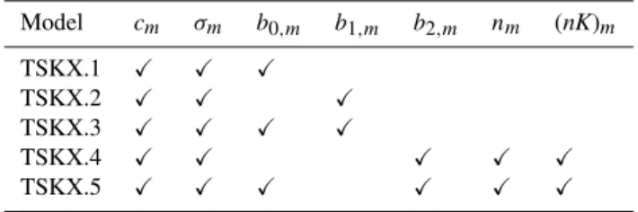
Table 1.Parameters involved in the TSK rainfall-runoff fuzzy mod-els proposed by Jacquin and Shamseldin (2006).
Model cm σm b0,m b1,m b2,m nm (nK)m TSKX.1 X X X
TSKX.2 X X X
TSKX.3 X X X X
TSKX.4 X X X X X
TSKX.5 X X X X X X
polynomials on the most recent normalized rainfall values
Pjn, which include a free termb0,min addition to first-order terms. These fuzzy models allow a different pulse response function for each rulem, characterized by gamma distribu-tion parametersnmand (nK)mthat define the pulse response ordinateshj,m.
The sensitivity of the parameters of fuzzy models TSK1.5 and TSK2.5 is studied, in order to establish whether the pa-rameters associated with a particular model component (e.g. the free terms in the rule consequents) are not important in determining the model performance. As mentioned earlier in the introduction, this situation would indicate that these pa-rameters can be excluded from the search of the behavioural regions of the parameter space in a model calibration prob-lem, by assigning them convenient values within their feasi-ble ranges (Saltelli et al., 2004). In the case of the fuzzy mod-els described here, this could be equivalent to considering a simpler model structure (e.g. fuzzy model TSK1.3 instead of TSK1.5), by removing the unimportant model component. The analysis is performed on fuzzy models with three rules, i.e. the same number of rules used in the study by Jacquin and Shamseldin (2006).
4 Methodology
4.1 Catchments and data
The data sets used in this study were obtained from the catch-ment database available at the Departcatch-ment of Engineering Hydrology, National University of Ireland, Galway. These data consist of daily averaged values of precipitation and daily average discharge at the catchment’s outlet. Table 2 shows the location of the catchments and the length of the data sets. The rainfall-runoff relationship of three of the test catchments, namely Sunkosi-1, Yanbian and Brosna, is af-fected by significant seasonal effects; in the case of the re-maining catchments, intrinsic non-linearity due to changes in soil moisture contents has greater importance. The catch-ments did not have hydrologically significant artificial struc-tures or human intervention at the time when the measure-ments were made.
As shown in Table 2, the available data are divided into a calibration and a verification period for split-record simu-lations. In general, the calibration and the verification data
from a same catchment have similar statistics (see Jacquin and Shamseldin, 2006). However, the variability of the cali-bration data of Bird Creek and Wollombi Brook is more pro-nounced than that of the corresponding verification data. In particular, the standard deviations of the discharge calibra-tion data of these latter catchments are much higher than in verification, even though the calibration and the verification discharge data have similar means. The data used for the split sampling tests are considered to be sufficiently long and have enough information contents, including a wide range of hydrological conditions.
4.2 Measures of model performance
The sensitivity of the parameters of the fuzzy models TSK1.5 and TSK2.5 with respect to the model performance is anal-ysed in terms of several measures of goodness of fit, assess-ing different aspects of the agreement between the observed and the simulated hydrograph. Each performance measure represents an output quantityY, whose variability (with re-spect to the parameters of the model) is to be examined.
The first performance measure under examination is the
R2 efficiency criterion of Nash and Sutcliffe (1970), given by the following expression
R2=MSE0−MSE MSE0
, (20)
where the initial mean squared error MSE0 corresponds to
the mean of the squares of the differences between the ob-served discharges and the long term mean during the cali-bration period. The mean squared error MSE is calculated as the mean of the squares of the differences between the model estimates and the observed discharges. The model ef-ficiencyR2is a decreasing function of the MSE, achieving a maximum value of unity if the model discharge estimates perfectly fit the observed discharges.
Another measure of goodness of fit used in this study is the deviation of runoff volumes, or relative error of the volu-metric fit (REVF), given by
REVF=1− PQ
i∗ PQ
i
, (21)
whereQi∗andQirepresent the model estimated and the ob-served discharge, respectively, at time stepi. Positive REVF values indicate underestimation of discharge volumes, while negative REVF values are obtained when volumes are being overestimated.
The last measure of model performance considered in this study is the average relative error to the peak (REP), given by
REP= Np
X
i=1
|Qpi−Qpi∗| NpQpi
Table 2.Location of the catchments and length of the data sets used in the experiments, including the definition of calibration and verification periods for split sampling tests.
Catchment Country Noof years Calibration period Verification period in data set
starting date Noof years starting date Noof years
Sunkosi-1 Nepal 8 1 Jan 1975 6 1 Jan 1981 2 Yanbian Central China 8 1 Jan 1978 6 1 Jan 1984 2 Shiquan-3 Central China 8 1 Jan 1973 6 1 Jan 1979 2 Brosna Central Ireland 10 1 Jan 1969 8 1 Jan 1977 2 Bird Creek Oklahoma, USA 8 1 Jan 1955 6 1 Jan 1961 2 Wollombi Brook New Sout Wales, Australia 5 1 Jan 1963 4 1 Jan 1967 1
Table 3.Performance statistics of the fuzzy models TSK1.5 and TSK2.5.
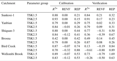
Catchment Parameter group Calibration Verification
R2∗ REVF REP R2∗ REVF REP Sunkosi-1 TSK1.5 0.88 0.00 0.21 0.84 0.21 0.32 TSK2.5 0.93 0.00 0.15 0.91 0.17 0.23 Yanbian TSK1.5 0.79 0.00 0.29 0.75 0.02 0.33 TSK2.5 0.84 −0.01 0.26 0.79 0.09 0.31 Shiquan-3 TSK1.5 0.88 0.00 0.44 0.77 −0.31 0.50 TSK2.5 0.84 −0.12 0.41 0.36 −0.39 0.67 Brosna TSK1.5 0.42 0.00 0.42 0.49 0.14 0.45 TSK2.5 0.79 0.00 0.26 0.87 0.08 0.26 Bird Creek TSK1.5 0.87 −0.07 0.74 0.13 −0.19 0.84 TSK2.5 0.70 −0.32 0.88 −0.61 −0.88 0.89 Wollombi Brook TSK1.5 0.89 −0.07 0.53 0.73 −0.79 1.69 TSK2.5 0.83 −0.12 0.53 −0.26 −0.50 0.63
∗R2values taken from the study by Jacquin and Shamseldin (2006).
model estimated discharge for the same time step as Qpi. The REP would be equal to zero in the ideal case of a per-fect estimation of all the selected flow peaks; increasing REP values indicate deterioration in the ability of the model to es-timate the peak discharges. In this study, the discharge peaks retained for the calculation of the REP values are those ex-ceeding the 90% of the calibration discharge data.
Table 3 shows the model performance statistics R2, REVF and REP of the fuzzy models TSK1.5 and TSK2.5, as calibrated by Jacquin and Shamseldin (2006). The fuzzy model TSK2.5 outperforms the fuzzy model TSK1.5 in terms of efficiency values R2, when applied in the catchments whose rainfall-runoff relationship has a seasonal nature (i.e. Sunkosi-1, Yanbian and Brosna); but, this situa-tion is reversed in the remaining catchments (i.e. Shiquan-3, Bird Creek and Wollombi Brook). In the non-seasonal
Table 4. Feasible ranges of the parameters of the fuzzy models TSK1.5 and TSK2.5.
Para- Lower Upper Description meter bound bound
cm 0 1 Centers of the antecedent fuzzy sets
σm 0.02 0.25 Spreads of the antecedent fuzzy sets
b0,m −1.315 1.456∗ Free terms in the
−0.162 0.641∗∗ consequent polynomials
b2,m 0 Pmax/Qmax Coefficients of first-order terms in the consequent polynomials
nm 0.5 10 Gamma distribution parameters describing the pulse responses of the rule consequents
(nK)m 0.5 30 Gamma distribution parameters describing the pulse responses of the rule consequents
∗Bounds applicable to TSK1.5.∗∗Bounds applicable to TSK2.5.
4.3 Computational experiments 4.3.1 Application of the RSA method
A random sample of 40 000 parameter sets is generated, both for the fuzzy model TSK1.5 and for TSK2.5. The feasi-ble space for sample generation is defined by the parame-ter bounds established in Table 4. Except in the case of the free termsb0,m, these bounds are the same as those imposed by Jacquin and Shamseldin (2006) for the calibration of the fuzzy models. In the case of the free termsb0,m, whose val-ues were not bounded during the calibration of the fuzzy models, the bounds shown in Table 4 are defined in such a manner that they are 50% wider than the range of b0,m values estimated by calibration of TSK1.5 and TSK2.5 for the test catchments. The performance of the fuzzy models is evaluated using the measures of goodness of fit indicated in Sect. 4.2. Probability distribution plots, produced using the software MCAT (Wagener and Kollat., 2007), are used for visually detecting sensitive parameters in the manner ex-plained in Sect. 2.2.1.
4.3.2 Application of the SVD method
The SVD method is applied by splitting the model parame-ters in groups, with the purpose of clearly highlighting the importance of each model component in the performance of the fuzzy models. The groups considered are: 1) antecedent centres cm, 2) antecedent spreads σm, 3) polynomial free termsb0,m, 4) polynomial coefficientsb2,m, 5) gamma dis-tribution parametersnm, and 6) gamma distribution param-eters (nK)m. In this case, the first-order effect of a group estimates to what extent the parameters in the group affect the model performance, excluding the effect of interactions with parameters outside the group. Similarly, the total ef-fect sensitivity index of a group of parameters provides an estimation of the overall importance of the group in the per-formance of the fuzzy models, including interactions with parameters outside the group. The samples of model param-eters and the sensitivity indices of the groups of paramparam-eters defined above are obtained with the sensitivity analysis soft-ware SIMLAB2.2 (European Union Joint Research Centre, 2004), using the Extended FAST sampling method (Saltelli et al., 1999). The bounds used for producing the samples of parameter sets are the same as those specified above for the case of the RSA method. The number of parameter sets in the sample is 9750.
5 Results
5.1 RSA results
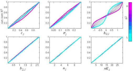
As examples of the application of the method, Figs. 1 and 2 show the results of RSA when applied to the fuzzy models TSK1.5 and TSK2.5, respectively, in the Sunkosi-1 catch-ment. In both figures, the model performance is evaluated using the efficiency criterionR2. Only the plots correspond-ing to one fuzzy rule are shown, but similar ones are obtained for the remaining rules. From the analysis of Fig. 1, it can be concluded that the model efficiencyR2of the fuzzy model TSK1.5 when applied in the Sunkosi-1 catchment is sensi-tive to changes in the parameters cm,σm and, particularly, b0,m. The remaining parameters of TSK1.5 are either non-important for determining the efficiencyR2, or their influ-ence arises from interactions that are not accounted for by the RSA method. Similarly, Fig. 2 shows that the model ef-ficiency R2 of the fuzzy model TSK2.5 is sensitive to the values taken by the parameters σm, b0,m andb2,m. In this case, the RSA method does not reveal any sensitivity of the model efficiencyR2with respect to the parameterscm, nm andnKm.
Fig. 1.Results of RSA method when applied to the fuzzy model TSK1.5 in the Sunkosi-1 catchment, using the efficiency criterionR2as a measure model performance.
Fig. 2.Results of RSA method when applied to the fuzzy model TSK2.5 in the Sunkosi-1 catchment, using the efficiency criterionR2as a measure model performance.
patterns in both periods. It can be observed that parameter sensitivities of fuzzy models TSK1.5 and TSK2.5 differ, and that the sensitivity of the parameters of these fuzzy models depends on the type of catchment (seasonal or non-seasonal) where the models are applied. For example, the performance of TSK1.5 does not seem to be greatly affected by univariate changes in the parametersb2,m(see Fig. 1). In the case of the fuzzy model TSK2.5, however, the values of all three mea-sures of model performance are sensitive to the parameters
b2,m, although only when TSK2.5 is applied in the seasonal catchments (see Fig. 2).
Table 5 also shows that the sensitivity of a parameter de-pends on the measure of model performance being consid-ered. Comparison of the columns corresponding toR2 and
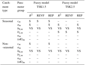
Table 5.Parameters of the fuzzy models deemed sensitive or very sensitive by the RSA method according to the measures of model performanceR2, REVF and REP.
Catch- Para- Fuzzy model Fuzzy model ment meter TSK1.5 TSK2.5 type group
R2 REVF REP R2 REVF REP
Seasonal cm S S S – – –
σm S – S S – S
b0,m VS VS VS VS VS VS
b2,m – – – S S S
nm – – – – – –
(nK)m – – – – – –
Non- cm S – S – – – -seasonal σm – – – – – –
b0,m VS VS VS VS VS VS
b2,m – – – – – –
nm – – – – – –
(nK)m – – – – – –
In any case, a feature that is common to all models, catch-ments and measures of model performance is that the RSA method shows the polynomial free termsb0,m as the most sensitive parameters. In addition to this, the gamma distribu-tion parametersnm and (nK)mare not revealed as sensitive in any fuzzy model or catchment.
5.2 SVD results
Tables 6 and 7 show the first-order effects for the fuzzy mod-els TSK1.5 and TSK2.5, respectively. Similarly, Tables 8 and 9 show the total effects corresponding to TSK1.5 and TSK2.5, respectively. Sensitivity indices values are shaded according to the following criteria: Values greater than 0.3, seen as an indication of high sensitivity, are shaded in dark gray; values between 0.15 and 0.3, interpreted as pointing out moderately sensitive parameters, are shaded in light gray; values between 0.02 and 0.15, seen as indicating parameters with a modest (but non-negligible) sensitivity are not shaded; finally, values smaller than 0.02, which are considered negli-gible, are highlighted in yellow. It seems important to point out that the sensitivity indices obtained for the calibration and the verification period are consistently close, which sug-gests that the results obtained in this analysis are independent on the period of data used for evaluation. The following dis-cussion gives the conclusions obtained from the analysis of Tables 6 to 9, according to the criteria outlined in Sect. 2.2.2. 5.2.1 First-order effects
As explained in Sect. 2.2.2, the first-order effect of a group of parameters represents the sensitivity of the quantityY un-der examination to changes in the parameters of the group, without considering the effect of interactions with
parame-ters outside the group. Except in the case where the interac-tion structure is such that its effects can be detected through RSA, the results of the RSA method provide similar informa-tion concerning the sensitivity of parameters. Therefore, it is not surprising that the analysis of the first-order effects in Ta-bles 6 and 7 confirm the main results of the RSA method, pre-sented in the previous section. In the first place, the highest first-order effects in Tables 6 and 7 correspond to the group of parametersb0,m, which are the only parameters classified as very sensitive (VS) by the RSA method. In addition to this, the first-order effects of the groups of parameters clas-sified as sensitive (S) by the RSA method are lower than in the previous case, although generally non-negligible. Finally, the first-order effects of those groups of parameters for which the RSA method did not reveal any sensitivity are negligible in all cases.
5.2.2 Total effects
Recalling the discussion in Sect. 2.2.2, the total effect of a group of parameters measures the sensitivity of the model re-sponse to the parameters in the group, including possible in-teractions with parameters in other groups. Accordingly, the total effects shown in Tables 8 and 9 are necessarily higher than the first-order effects in Tables 6 and 7, which exclude the effect of interactions outside the group. These interac-tions with other groups are revealed by great differences be-tween the group’s total effects and first-order effects. The following discussion analyses the sensitivity of each group of parameters according to their total effects and the existence of interactions between groups.
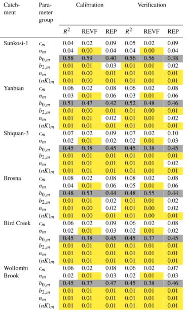
Table 6. First-order effect sensitivity indices of the parameters of the fuzzy model TSK1.5. Dark gray shading indicates values greater than 0.3 and light gray shading indicates values between 0.15 and 0.3. Values smaller than 0.02 are shaded in yellow.
Catch- Para- Calibration Verification ment meter
group
R2 REVF REP R2 REVF REP
Sunkosi-1 cm 0.04 0.02 0.09 0.05 0.02 0.09
σm 0.04 0.00 0.04 0.04 0.00 0.04
b0,m 0.58 0.59 0.40 0.56 0.56 0.38
b2,m 0.01 0.01 0.03 0.01 0.01 0.02
nm 0.01 0.00 0.01 0.01 0.01 0.01
(nK)m 0.01 0.00 0.01 0.01 0.01 0.01 Yanbian cm 0.06 0.02 0.08 0.06 0.02 0.08
σm 0.03 0.01 0.06 0.03 0.01 0.06
b0,m 0.51 0.47 0.42 0.52 0.48 0.46
b2,m 0.01 0.00 0.01 0.01 0.00 0.01
nm 0.01 0.01 0.02 0.01 0.01 0.02
(nK)m 0.01 0.01 0.01 0.01 0.01 0.01 Shiquan-3 cm 0.07 0.02 0.09 0.07 0.02 0.10
σm 0.02 0.01 0.02 0.02 0.01 0.03
b0,m 0.45 0.38 0.45 0.45 0.38 0.45
b2,m 0.01 0.01 0.01 0.01 0.01 0.01
nm 0.01 0.01 0.01 0.01 0.01 0.02
(nK)m 0.01 0.01 0.01 0.01 0.01 0.01 Brosna cm 0.08 0.02 0.08 0.08 0.02 0.08
σm 0.04 0.01 0.06 0.05 0.01 0.06
b0,m 0.48 0.53 0.44 0.48 0.55 0.44
b2,m 0.01 0.01 0.02 0.01 0.01 0.02
nm 0.01 0.00 0.02 0.01 0.00 0.02
(nK)m 0.01 0.00 0.01 0.01 0.00 0.01 Bird Creek cm 0.06 0.02 0.09 0.06 0.02 0.08
σm 0.02 0.01 0.03 0.02 0.01 0.02
b0,m 0.45 0.38 0.45 0.45 0.37 0.45
b2,m 0.01 0.01 0.01 0.01 0.01 0.01
nm 0.01 0.01 0.01 0.01 0.01 0.01
(nK)m 0.01 0.01 0.01 0.01 0.01 0.01 Wollombi cm 0.06 0.02 0.08 0.06 0.02 0.07 Brook σm 0.02 0.01 0.03 0.02 0.01 0.03
b0,m 0.45 0.37 0.47 0.45 0.38 0.46
b2,m 0.01 0.01 0.01 0.01 0.01 0.01
nm 0.01 0.01 0.01 0.01 0.01 0.01
(nK)m 0.01 0.01 0.01 0.01 0.01 0.01
TSK1.5, as the total effects of these groups are consistently small. More concretely, for all catchments and measures of model performance, the total effects of these groups do not exceed 0.14.
The total effects shown in Table 9 indicate that the free termsb0,m are the parameters with the highest influence in the performance of TSK2.5, as indicated by all three mea-sures of model performance and in all the catchments. Un-like the case of TSK1.5, the total effects of the antecedent centrescmare generally low. However, a high sensitivity is seen when the model TSK2.5 is applied in the seasonal catch-ments and the measure of model performance REP is used, in which case the total effects of the centrescmrange between
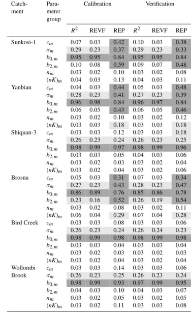
Table 7. First-order effect sensitivity indices of the parameters of the fuzzy model TSK2.5. Dark gray shading indicates values greater than 0.3 and light gray shading indicates values between 0.15 and 0.3. Values smaller than 0.02 are shaded in yellow.
Catch- Para- Calibration Verification ment meter
group
R2 REVF REP R2 REVF REP
Sunkosi-1 cm 0.01 0.00 0.10 0.01 0.00 0.07
σm 0.03 0.00 0.09 0.04 0.00 0.06
b0,m 0.59 0.62 0.22 0.57 0.63 0.27
b2,m 0.03 0.04 0.08 0.01 0.03 0.08
nm 0.00 0.00 0.01 0.00 0.00 0.01
(nK)m 0.00 0.00 0.02 0.00 0.00 0.01 Yanbian cm 0.01 0.00 0.09 0.01 0.00 0.09
σm 0.02 0.00 0.10 0.02 0.00 0.10
b0,m 0.62 0.64 0.32 0.62 0.64 0.30
b2,m 0.01 0.02 0.07 0.01 0.02 0.06
nm 0.00 0.00 0.01 0.00 0.00 0.01
(nK)m 0.00 0.00 0.02 0.00 0.00 0.03 Shiquan-3 cm 0.00 0.00 0.01 0.00 0.00 0.01
σm 0.02 0.00 0.01 0.02 0.00 0.02
b0,m 0.64 0.66 0.58 0.64 0.66 0.53
b2,m 0.00 0.00 0.01 0.00 0.00 0.01
nm 0.00 0.00 0.00 0.00 0.00 0.00
(nK)m 0.00 0.00 0.01 0.00 0.00 0.01 Brosna cm 0.00 0.00 0.06 0.01 0.00 0.08
σm 0.03 0.00 0.13 0.03 0.00 0.14
b0,m 0.53 0.58 0.25 0.50 0.57 0.23
b2,m 0.13 0.11 0.13 0.13 0.12 0.11
nm 0.00 0.00 0.01 0.00 0.00 0.01
(nK)m 0.01 0.01 0.07 0.02 0.01 0.05 Bird Creek cm 0.00 0.00 0.01 0.00 0.00 0.01
σm 0.01 0.00 0.01 0.01 0.00 0.01
b0,m 0.64 0.66 0.62 0.64 0.66 0.65
b2,m 0.00 0.00 0.00 0.00 0.00 0.00
nm 0.00 0.00 0.00 0.00 0.00 0.00
(nK)m 0.00 0.00 0.01 0.00 0.00 0.00 Wollombi cm 0.00 0.00 0.01 0.00 0.00 0.01 Brook σm 0.01 0.00 0.01 0.01 0.00 0.01
b0,m 0.64 0.66 0.53 0.64 0.66 0.64
b2,m 0.00 0.00 0.02 0.00 0.00 0.02
nm 0.00 0.00 0.00 0.00 0.00 0.00
(nK)m 0.00 0.00 0.03 0.00 0.00 0.02
Table 8. Total effect sensitivity indices of the parameters of the fuzzy model TSK1.5. Dark gray shading indicates values greater than 0.3 and light gray shading indicates values between 0.15 and 0.3.
Catch- Para- Calibration Verification ment meter
group
R2 REVF REP R2 REVF REP
Sunkosi-1 cm 0.51 0.32 0.54 0.55 0.35 0.53
σm 0.17 0.08 0.20 0.17 0.08 0.23
b0,m 0.94 0.98 0.91 0.94 0.98 0.91
b2,m 0.09 0.05 0.17 0.09 0.06 0.16
nm 0.12 0.07 0.10 0.13 0.07 0.10
(nK)m 0.08 0.07 0.10 0.08 0.07 0.11 Yanbian cm 0.62 0.44 0.49 0.61 0.43 0.45
σm 0.16 0.08 0.28 0.16 0.08 0.26
b0,m 0.93 0.98 0.87 0.93 0.98 0.88
b2,m 0.09 0.06 0.11 0.09 0.06 0.12
nm 0.13 0.08 0.12 0.13 0.08 0.11
(nK)m 0.08 0.08 0.09 0.08 0.08 0.09 Shiquan-3 cm 0.70 0.55 0.68 0.69 0.54 0.66
σm 0.16 0.07 0.17 0.16 0.07 0.19
b0,m 0.93 0.98 0.91 0.93 0.98 0.89
b2,m 0.10 0.07 0.09 0.10 0.07 0.09
nm 0.14 0.09 0.12 0.13 0.09 0.13
(nK)m 0.09 0.08 0.08 0.09 0.08 0.09 Brosna cm 0.55 0.37 0.44 0.54 0.34 0.45
σm 0.21 0.12 0.27 0.23 0.13 0.27
b0,m 0.89 0.98 0.87 0.88 0.97 0.88
b2,m 0.12 0.06 0.14 0.13 0.05 0.14
nm 0.12 0.06 0.11 0.12 0.06 0.12
(nK)m 0.09 0.07 0.11 0.09 0.07 0.11 Bird cm 0.69 0.55 0.67 0.70 0.55 0.69 Creek σm 0.16 0.07 0.17 0.16 0.07 0.16
b0,m 0.94 0.98 0.90 0.94 0.98 0.91
b2,m 0.10 0.07 0.09 0.10 0.07 0.09
nm 0.13 0.09 0.12 0.14 0.09 0.12
(nK)m 0.09 0.08 0.08 0.09 0.08 0.08 Wollombi cm 0.69 0.55 0.63 0.69 0.55 0.64 Brook σm 0.16 0.07 0.16 0.16 0.07 0.17
b0,m 0.94 0.98 0.91 0.94 0.98 0.91
b2,m 0.10 0.07 0.09 0.10 0.07 0.10
nm 0.13 0.09 0.12 0.13 0.09 0.12
(nK)m 0.09 0.08 0.09 0.09 0.08 0.10
6 Conclusions
This study has analysed the sensitivity of the parameters of the Takagi-Sugeno-Kang rainfall-runoff fuzzy models pro-posed by Jacquin and Shamseldin (2006). These models can be classified in two model types, each consisting of five model structures of increasing complexity. The fuzzy mod-els TSK1.5 and TSK2.5 are the most complex within types 1 and 2, respectively, and they include all the model compo-nents found in the simpler fuzzy models of the correspond-ing group. Two global sensitivity analysis methods were ap-plied, namely the RSA and SVD methods. In general, the
Table 9. Total effect sensitivity indices of the parameters of the fuzzy model TSK2.5. Dark gray shading indicates values greater than 0.3 and light gray shading indicates values between 0.15 and 0.3.
Catch- Para- Calibration Verification ment meter
group
R2 REVF REP R2 REVF REP
Sunkosi-1 cm 0.07 0.03 0.42 0.10 0.03 0.38
σm 0.29 0.23 0.37 0.29 0.23 0.33
b0,m 0.95 0.95 0.84 0.95 0.95 0.84
b2,m 0.10 0.08 0.59 0.09 0.07 0.48
nm 0.03 0.02 0.10 0.03 0.02 0.08
(nK)m 0.04 0.03 0.13 0.04 0.03 0.11 Yanbian cm 0.04 0.03 0.44 0.05 0.03 0.48
σm 0.28 0.23 0.41 0.27 0.23 0.39
b0,m 0.96 0.98 0.84 0.96 0.97 0.84
b2,m 0.06 0.05 0.43 0.06 0.05 0.46
nm 0.03 0.02 0.10 0.03 0.02 0.12
(nK)m 0.03 0.03 0.18 0.03 0.03 0.18 Shiquan-3 cm 0.03 0.03 0.12 0.03 0.03 0.18
σm 0.26 0.23 0.24 0.26 0.23 0.25
b0,m 0.98 0.99 0.97 0.98 0.99 0.96
b2,m 0.03 0.03 0.05 0.04 0.03 0.06
nm 0.03 0.02 0.03 0.03 0.02 0.04
(nK)m 0.03 0.02 0.04 0.03 0.02 0.06 Brosna cm 0.05 0.03 0.31 0.07 0.03 0.34
σm 0.27 0.23 0.43 0.28 0.23 0.47
b0,m 0.86 0.89 0.76 0.85 0.86 0.78
b2,m 0.23 0.16 0.52 0.26 0.19 0.54
nm 0.03 0.02 0.08 0.03 0.02 0.11
(nK)m 0.06 0.04 0.29 0.07 0.04 0.28 Bird Creek cm 0.03 0.03 0.08 0.03 0.03 0.06
σm 0.26 0.23 0.24 0.26 0.24 0.23
b0,m 0.98 0.99 0.98 0.98 0.99 0.98
b2,m 0.03 0.03 0.04 0.03 0.03 0.04
nm 0.03 0.02 0.03 0.03 0.02 0.03
(nK)m 0.03 0.02 0.04 0.03 0.02 0.04 Wollombi cm 0.03 0.03 0.14 0.03 0.03 0.06 Brook σm 0.26 0.23 0.25 0.26 0.23 0.24
b0,m 0.98 0.99 0.93 0.97 0.99 0.95
b2,m 0.04 0.03 0.10 0.04 0.03 0.07
nm 0.03 0.02 0.05 0.03 0.02 0.05
(nK)m 0.03 0.02 0.11 0.03 0.03 0.08
RSA method has the disadvantage of not being able to detect sensitivities arising from parameter interactions. By contrast, the SVD method is suitable for analysing models where the model response surface is expected to be affected by interac-tions at a local scale and/or local optima, such as the case of the rainfall-runoff fuzzy models of Jacquin and Sham-seldin (2006).
parameter sensitivities vary according to the statistic chosen for evaluating model performance. For example, the total effects of the antecedent centrescm in the performance of TSK2.5 are generally low, but the statistic REP (reflecting the relative error to the peak) was found to be very sensitiv-ity to these parameters in the case of the seasonal catchments. These results are in agreement with previous research, show-ing that the sensitivity of the parameters of a rainfall-runoff model is dependent on the catchment’s hydroclimatic charac-teristics and on the measure of model performance (Tang et al., 2007; van Werkhoven et al., 2008). However, broad gen-eralizations on parameter sensitivities of the fuzzy models TSK1.5 and TSK2.5 can still be attempted, with the purpose of facilitating the calibration process by identifying the pa-rameters with the highest influence in the model’s goodness of fit, and those which can be fixed without important loss of accuracy in the discharge estimates.
In the case of the fuzzy model TSK1.5, it was found that the performance of the model is quite sensitive to the an-tecedent centrescm, although most of this influence is due to interactions with the parametersb0,m. It was also observed that the antecedent spreadsσmhave a moderate importance in determining the model performance of TSK1.5. Similarly, it was observed that the antecedent parameterscm and σm generally do not have a high influence in the performance of TSK2.5. These situations imply that the actual definition of the antecedent fuzzy sets is not, on its own, a determinant factor for the goodness of fit of the fuzzy models TSK1.5 and TSK2.5. It would be possible to fix the antecedent pa-rameters prior to the calibration of the fuzzy models without an important deterioration of model performance, provided that the values of the remaining parameters are conveniently adjusted.
It was also observed that, in general, the coefficientsb2,m do not greatly affect the performance of TSK1.5 and TSK2.5. By contrast, the free termsb0,mwere identified as the param-eters with the highest influence in the performance of TSK1.5 and TSK2.5. Moreover, these parameters exhibit quite high (and also the highest) first-order effects in all cases, mod-ifying the model performance independently of interactions with parameters in other groups. As pointed out by Saltelli et al. (2004), the identification of appropriate values for param-eters with a high first-order effect should be a priority dur-ing the process of model calibration. Nevertheless, Jacquin and Shamseldin (2006) showed that removing the parameters
b0,m, by moving from the fuzzy models TSKx.3 and TSKx.5 to the simpler TSKx.2 and TSKx.4, respectively, does not have a significant impact in the performance of the opti-mised rainfall-runoff fuzzy model. This situation indicates that finding the “true” values of the free termsb0,mdoes not necessarily improve the goodness of fit, as long as these pa-rameters are all assigned zero values.
This apparent contradiction between the findings of Jacquin and Shamseldin (2006) and the results of the sen-sitivity analysis presented in this study can be explained
af-ter a more careful consideration of the facts. First, the large total and first-order effects of the parametersb0,m indicate that allowing a free variation of these parameters across their feasible range does produce important changes in the good-ness of fit of the fuzzy models TSK1.5 and TSK2.5. In fact, assigning very inappropriate values to these parameters may result in an important deterioration of model performance; for example, assigning highly negative values to the param-etersb0,min all of the rules would result in highly negative discharge estimates in cases where the most recent rainfall segment is null. However, it is still possible that a relatively good (and nearly optimal) model response can be obtained by fixing the values of the parametersb0,mas zero and cali-brating the remaining model parameters accordingly.
Finally, the results of this study indicate that the gamma distribution parameters nm and (nK)mare almost unimpor-tant in determining the goodness of fit of the fuzzy models TSK1.5 and TSK2.5. These results are in agreement with the findings of Jacquin and Shamseldin (2006), in the sense that allowing a different pulse response for each rule consequent (i.e. moving from the fuzzy models TSKx.2 and TSKx.3 to TSKx.4 and TSKx.5, respectively) does not necessarily im-prove the performance of the optimised fuzzy model. In or-der to reduce the dimensionality of the optimisation problem associated with the calibration of the model, these param-eters could be excluded from the search of the behavioural regions of the parameter space, by assigning to them fixed values within their feasible ranges. For example, the values of the parametersnmand (nK)mof all the fuzzy rules could be given the same values as those of the auxiliary SLM. As seen in Sect. 3.2, this would be equivalent to abandoning the models TSK1.5 and TSK2.5 in favour of the more parsimo-nious TSK1.3 and TSK2.3, respectively.
Further work could explore the application of the GSA methods applied in this paper to other hydrological models based on soft computing methods. For example, it would be convenient to perform sensitivity analysis of other fuzzy model structures. Similarly, it would also be interesting to use this methods method for investigating the relative im-portance of the parameters of typical neural network based rainfall-runoff models. The application of the method would allow identifying those parameters whose values can be fixed without important deterioration in model performance and those parameters whose appropriate calibration is most im-portant.
Acknowledgements. This research was supported by FONDECYT, Research Grant 11070130. We would also like to express our gratitude to Kieran M. O’Connor from the National University of Ireland, Galway, for providing the data used in this study. Finally, we would like convey our appreciation to the editor Erwin Zehe and the anonymous referees for their constructive criticisms, which have helped us to improve the quality of the manuscript.
References
B´ardossy, A. Bronstert, A., and Merz, B.: 1-, 2- and 3-dimensional modelling of water movement in the unsaturated soil matrix us-ing a fuzzy approach, Adv. Water Resour., 18(4), 237–251, 1995. B´ardossy, A. and Disse, M.: Fuzzy Rule-Based Models for
Infiltra-tion, Water Resour. Res., 29(2), 373–382, 1993.
B´ardossy, A., Mascellani, G., and Franchini, M.: Fuzzy unit hydrograph, Water Resour. Res., 42(2), W02401, doi:10.1029/2004WR003751, 2006.
Beven, K. J.: Rainfall-Runoff Modelling: The Primer, John Wiley & Sons, Chichester, 360 pp., 2001.
Castaings, W., Dartus, D., Honnorat, M., Le Dimet, F. X., Loukili, Y., and Monnier, J.: Automatic differentiation: a tool for varia-tional data assimilation and adjoint sensitivity analysis for flood modelling, in: Automatic Differentiation: Applications, Theory, and Tools, edited by: B¨ucker, H. M., Corliss, G., Hovland, P., Naumann, U., and Norris, B., Springer, Chicago, 249–262, 2005. Chan, K., Tarantola, S., Saltelli, A., and Sobol, I. M.: Variance-based methods, in: Sensitivity Analysis, edited by: Saltelli, A., Chan, K., and Scott, E. M., John Wiley & Sons, Chichester, 167– 197, 2000.
Cukier, R. I., Fortuin, C. M., Shuler, K. E., Petschek, A. G., and Schaibly, J. H.: A Study of the Sensitivity of Coupled Reaction Systems to Uncrtainties in Rate Coefficients: I Theory, J. Chem. Phys., 59(8), 3873–3878, 1973.
Cukier, R. I., Levine, H. B., and Shuler, K. E.: Nonlinear sensitivity analysis of multiparameter model systems, J. Comput. Phys., 26, 1–42, 1978.
Demicco, R. and Klir, G.: Fuzzy Logic in Geology, Academic Press, Amsterdam, 347 pp., 2004.
Dou, X., Wouldt, W., and Bogardi, I.: Fuzzy rule-based approach to describe solute transport in the unsaturated zone, J. Hydrol., 220, 74–85, 1999.
European Union Joint Research Centre: SIMLAB: Simulation En-vironment for Uncertainty and Sensitivity Analysis (version 2.2), Applied Statistics Sector, Institute for Systems, Informatics and Safety, European Union Joint Research Centre, Ispra, Italy, 2004. Fieberg, J. and Jenkings, K. J.: Assessing uncertainty in ecologi-cal systems using global sensitivity analyses: a case example of simulated wolf reintroduction effects on elk, Ecol. Model., 187, 259–280, 2005.
Francos, A., Elorzab, F. J., Bouraouia, F., Bidoglioa, G., and Galbi-atia, L.: Sensitivity analysis of distributed environmental simula-tion models: understanding the model behaviour in hydrological studies at the catchment scale, Reliab. Eng. Syst. Safe., 205–218, 2003.
Gupta, V. K. and Sorooshian, S.: The automatic calibration of con-ceptual catchment models using derivative-based optimization algorithms, Water Resour. Res., 21(4), 473–485, 1985.
Homma, T. and Saltelli, A.: Importance measures in global sensi-tivity analysis of model output, Reliab. Eng. Syst. Safe, 52, 1–17, 1996.
Hornberger, G. M. and Spear, R. C.: An approach to the preliminary analysis of environmental systems, J. Environ. Manage., 12, 7– 18, 1981.
Hundecha, Y. and B´ardossy, A.: Modeling of the effect of land use changes on the runoff generation of a river basin through pa-rameter regionalization of a watershed model, J. Hydrol., 292, 281–295, 2004.
Hundecha, Y., B´ardossy, A., and Theisen, H.-W.: Development of a fuzzy logic-based rainfall-runoff model, Hydrolog. Sci. J., 46(3), 363–376, 2001.
Jacquin, A. P. and Shamseldin, A. Y.: Development of rainfall-runoff models using Takagi-Sugeno-Kang fuzzy inference sys-tems, J. Hydrol., 329, 154–173, 2006.
Jacquin, A. P. and Shamseldin, A. Y.: Development of a possi-bilistic method for the evaluation of predictive uncertainty in rainfall-runoff modelling, Water Resour. Res., 43(4), W04425, doi:10.1029/2006WR005072, 2007.
Kanso, A., Chebboa, G., and Tassina, B.: Application of MCMC-Global sensitivity analysis method for model calibration to ur-ban runoff quality model, in: Sensitivity Analysis of Model Out-put, edited by: Hanson, K. M. and Hemez, F. M., Los Alamos National Laboratory, 17–26, available at: http://library.lanl.gov, 2005.
McIntyre, N. R., Wagener, T., Wheater, H., and Chapra, S. C.: Risk-based modelling of surface water quality: a case study of the Charles River, Massachussetts, J. Hydrol., 274, 225–247, 2003. Mein, R. G. and [yellow], B. M.: Sensitivity of optimized
param-eters in watershed models, Water Resour. Res., 14(2), 299–303, 1978.
Mertens, J., Madsen, H., Kristensen, M., Jacques, D., and Feyen, J.: Sensitivity of soil parameters in saturated zone modelling and the relation between effective, laboratory and in situ estimates, Hy-drol. Process., 19(8), 1611–1633, doi:10.1002/hyp.5591, 2005. Morris, M. D.: Factorial sampling plans for preliminary
computa-tional experiments, Technometrics, 33(2), 161–074, 1991. Nandakumar, N. and Mein, R. G.: Uncertainty in rainfall-runoff
model simulations and the implications for predicting the hydro-logic effects of land-use change, J. Hydrol., 192, 211–232, 1997. Nash, J. E.: The form of the instantaneous unit hydrograph, IASH
Publication, 45(3), 114–118, 1957.
Nash, J. E. and Foley, J. J.: Linear models of rainfall-runoff sys-tems, in: Rainfall-runoff relationships, Proceedings of the Inter-national Symposium on Rainfall-Runoff Modeling, Mississippi State University, USA, May 1981, 51–66, 1982.
Nash, J. E. and Sutcliffe, J. V.: River flow forecasting through con-ceptual models, Part I – A discussion of principles, J. Hydrol., 10, 282–290, 1970.
O’Connor, K. M.: River flow forecasting, in: River Basin Mod-elling for Flood Risk Mitigation, edited by: Knight, D. W. and Shamseldin A. Y., Taylor & Francis, London, 197–213, 2005. ¨
Ozelkan, E. C. and Duckstein, L.: Fuzzy conceptual rainfall-runoff models, J. Hydrol., 253, 41–68, 2001.
¨
Ozelkan, E. C., Galambosi, A., Duckstein, L., and B´ardossy, A.: A multi-objective fuzzy classification of large scale atmospheric circulation patterns for precipitation modelling, Appl. Math. Comput., 91, 127–142, 1998.
Pappenberger, F., Beven, K. J., Ratto, M., and Matgen, P.: Multi-method global sensitivity analysis of flood inundation models, Adv. Water Resour., 31(1), 1–14, 2008.
Pongracz, R., Bartholy, J., and Bogardi, I. Fuzzy rule-based predic-tion of monthly precipitapredic-tion, Phys. Chem. Earth Pt. B, 26(9), 663–667, 2001.
http://www.hydrol-earth-syst-sci.net/11/1249/2007/.
Saltelli, A., Ratto, M., Andres, T., Campolongo, F., Cariboni, J., Gatelli, D., Saisana, M., and Tarantola, S.: Global Sensitivity Analysis: The Primer, John Wiley & Sons, Chichester, 292 pp., 2008.
Saltelli, A., Tarantola, S., and Campolongo, F.: Sensitivity analysis as an ingredient of modelling, Stat. Sci., 15(4), 377–395, 2000. Saltelli, A., Tarantola, S., Campolongo, F., and Ratto, M.:
Sensitiv-ity analysis in practice: A guide to assessing scientific models, John Wiley & Sons, Chichester, 219 pp., 2004.
Saltelli, A., Tarantola, S., and Chan, K.: A quantitative, model inde-pendent method for global sensitivity analysis of model output, Technometrics, 41(1), 39–56, 1999.
Seibert, J.: Regionalization of parameter of a conceptual rainfall-runoff model, Agr. Forest Meteorol., 98–99, 279–293, 1999. Sobol, I. M.: Sensitivity analysis for non-linear mathematical
mod-els, Mathematical Modelling and Computational Experiments, 1(4), 407–414, 1993.
Sorooshian, S. and Gupta, V. K.: Model calibration, in: Conceptual Models of Watershed Hydrology, edited by: Singh, V. P., Water Resources Publications, Colorado, 23–67, 1995.
Spear, R. C. and Hornberger, G. M.: Eutrophication in Peel Inlet II: Identification of critical uncertainties via generalised sensitivity analysis, Water Resour. Res., 14, 43–49, 1980.
Sugeno, M. and Kang, G. T.: Structure identification of fuzzy model, Fuzzy Set. Syst., 28, 15–33, 1988.
Takagi, T. and Sugeno, M.: Fuzzy identification of systems and its application to modeling and control, IEEE T. Syst. Man Cyb., SMC-15(1), 116–132, 1985.
Tang, Y., Reed, P., Wagener, T., and van Werkhoven, K.: Comparing sensitivity analysis methods to advance lumped watershed model identification and evaluation, Hydrol. Earth Syst. Sci., 11, 793– 817, 2007, http://www.hydrol-earth-syst-sci.net/11/793/2007/. Vernieuwe, H., Georgieva, O., De Baets, B., Pauwels, V. R. N.,
Verhoest, N. E. C., and De Troch, F. P.: Comparison of data-driven Takagi-Sugeno models of rainfall-discharge dynamics, J. Hydrol., 302, 173–186, 2005.
Wagener, T., Boyle, D. P., Lees, M. J., Wheater, H. S., Gupta, H. V., and Sorooshian, S.: A framework for development and applica-tion of hydrological models, Hydrol. Earth Syst. Sci., 5, 13–26, 2001, http://www.hydrol-earth-syst-sci.net/5/13/2001/.
Wagener, T. and Kollat, J.: Numerical and visual evaluation of hydrological and environmental models using the Monte Carlo analysis toolbox, Environ. Modell. Softw., 22(7), 1021–1033, 2007.
Wagener, T., Wheater, H. S., and Gupta, H. V.: Identification and evaluation of watershed models, in: Calibration of Watershed Models, edited by: Duan, Q., Gupta, H. V., Sorooshian, S., Rousseau, A. N., and Turcotte, R., American Geophysical Union, Washington, 29–47, 2002.
Wang, X., Frankenberger, J. R., and Kladivko, E. J.: Uncertainties in DRAINMOD predictions of subsurface drain flow for and In-diana silt loam using the GLUE methodology, Hydrol. Process., 20(14), 3069–3084, doi:10.1002/hyp.6080, 2006.
van Werkhoven, K., Wagener, T., Reed, P., and Tang, Y.: Characterization of watershed model behavior across a hy-droclimatic gradient, Water Resour. Res., 44, W01429, doi:10.1029/2007WR006271, 2008.
Xiong, L. and O’Connor, K. M.: Analysis of the response surface of the objective function by the optimum parameter curve: How good can the optimum parameter values be?, J. Hydrol., 234, 187–207, 2000.
Yu, P.-S., and Yang, T. C.: Fuzzy multi-objective function for rainfall-runoff model calibration, J. Hydrol., 238, 1–14, 2000. Zadeh, L. A.: Fuzzy Sets, Inform. Control, 8(3), 338–353, 1965. Zehe, E., Becker, R., B´ardossy, A. and Plate, E. Uncertainty of
sim-ulated catchment runoff response in the presence of threshold processes: Role of initial soil moisture and precipitation, J. Hy-drol., 315, 183–202, 2005.
Zehe, E. and Bl¨oschl, G.: Predictability of hydrologic response at the plot and catchment scales: The role of initial conditions, Wa-ter Resour. Res., 40(10), W10202, doi:10.1029/2003WR002869, 2004.
Zehe, E., Singh, A. K., and B´ardossy, A.: Modelling of monsoon rainfall for a mesoscale catchment in North-West India I: assess-ment of objective circulation patterns, Hydrol. Earth Syst. Sci., 10, 797–806, 2006,