Vortex Dynamics Equation in Type-II Superconductors in a Temperature Gradient
R. Vega Monroy∗ and J. Sarmiento Castillo
Facultad de Ciencias B´asicas. Universidad del Atl´antico Km. 7, Via a Pto. Colombia, Barranquilla, Colombia
D. Puerta Torres
Facultad de Ciencias Exactas. Universidad de Cartagena Plaza de la Artiller´ıa N. 30-84, Cartagena, Colombia
(Received on 27 August, 2010)
In this work we determined a vortex dynamics equation in a temperature gradient in the frame of the time dependent Ginzburg-Landau equation. In this sense, we derived a local solvability condition, which governs the vortex dynamics. Also, we calculated the explicit form for the force coefficients, which are the keys for the understanding of the balance equation due to vortex interactions with the environment.
Keywords: Type-II Superconductors; Vortex Equation; Vortex Balance Equation.
1. INTRODUCTION
In type-II superconductors, the vortices are the ones in charge for the magnetic properties of these systems since ev-ery vortex carries a magnetic flux quantum. In the last years the interest in the vortex motion is associated to many non peculiar properties in HTSC not found in conventional type-II superconductors. In particular, one of the most important effects encountered in HTSC is the Hall anomaly [1,2]. In this sense, it is known that, under the action of the Lorentzs force vortices acquire a movement and therefore losses ap-pear in the superconducting state. The equation of motion, which governs the vortex dynamics in type-II superconduc-tors, has been subject to a great amount of works, which have helped us to understand this phenomenon in these systems. In addition, the interest in the vortex motion is emphasized by the responsibility of this dynamics in a great variety of transport phenomena in type II superconductors. Generally, the vortex dynamics has been considered on the hydrody-namical two fluid model [3,4], where the relative motion be-tween the superfluid and the vortex generates the Magnus force. Next, the normal component reacts to this motion, pro-ducing the longitudinal viscous drag force and the transver-sal Iordanski’s force, which are the two components of the medium force. An attempt to describe the vortex dynamics was done by Dorsey [5] in the frame of the time dependent Ginzburg-Landau equation following previous developments of Gorkov and Kopnin [6]. In this work, Dorsey formulates a solubility condition through with a vortex equation can be obtained. Today, there are several attempts to construct a uni-fied theory about the vortex motion. Some approximations use the sophisticated many body formalism [7,8,9]. Other authors apply a simpler theory based on the kinetic Boltz-mann equation to study the dynamic behavior of the vortex structures [10], but so far the vortex dynamics is an open question for the solid state physics community. The purpose of the present work is to contribute to a better understanding of the fascinating phenomenon of the vortex motion. In this connection, the goal of this paper is to determine a vortex dynamics equation in a temperature gradient in the frame of the time dependent Ginzburg-Landau equation. Such kind
∗Electronic address:[email protected]
of equation has been introduced in a heuristic way in many works [11] to satisfy experimental data [12,13,14].
The paper is organized as follows: In Section 2, we have obtained the basics equations of the work. In Section 3, some dynamic coefficients are calculated and finally in Section 4 we summarized the main results.
2. BASIC EQUATIONS
The present analysis follows the works done by Dorsey [5] in order to obtain the equation, which describes the vortex dynamics. Let us write the dimensionless time dependent Ginzburg-Landau equation for the complex order parameter in the form:
γ
∂
∂t+iφ
ψ=
"~
∇ κ−i~A
#2
ψ+ψ− |ψ|2ψ. (1)
In the above equationγis the dimensionless relaxation time, κis the Ginzburg-Landau parameter,Φand~Aare the electric potential and the magnetic vector respectively. The order pa-rameterψin terms of the amplitudef(~r,t)and the faseχ(~r,t) can be represented as follows ψ(~r,t) = f(~r,t)exp[iχ(~r,t)]. The relaxation time has a complex character and can be writ-ten
γ=γ1+iγ2.
The appearance of the imaginary part in the previous expres-sion is a necessary condition for the gauge invariance conser-vation of equation (1) [10]. Relaxation processes that entail to dispersion in the vortex dynamics are of two types: the first is associated to the Bardeen- Stephens mechanism of dissipation and the second process is an intrinsic relaxation mechanism that governs the approach of the order parame-ter to its equilibrium state due to variations in the chemical potential. This mechanism is associated to the change of the order parameter in time because the electrons are forced to pair and de-pair with respect to different potentials due to the vortex motion. In consequence, this processe is the respon-sible that the relaxation time acquires a complex character as was shown by Kopnin [10] and it is framed in the parameter γ2
γ2=−
~
whereνandµare the density of states and the chemical po-tential respectively. Introducingψ andγin the expression (1) and in addition, introducing the invariant forms for the magnetic vector and the scalar potential
~
Q=~A−1
κ~∇χ, P=Φ+ ∂χ
∂t, (2)
one can obtain two equations, the first for the real part and the other one for the imaginary part as follows:
γ1 ∂f
∂t −γ2f P= 1 κ2~∇
2f+Q2f
−f−f3, (3)
γ1f P−γ2 ∂f
∂t + 2 κQ~.~∇f+
f
κ~∇.~Q=0. (4) To form a closed system of equations, we need to derive an equation for the magnetic vector. In this connection, the di-mensionless equations for the superconducting and normal current are:
~ Js=
1
2κi(ψ∗~∇ψ−ψ~∇ψ∗)− |ψ| 2~A=
−f2~Q, (5)
~
Jn=σ(n)(− 1 κ~∇P−
∂~Q ∂t ) +
1 κb
(n)~∇T, (6)
whereσ(n) andb(n) are the electric and thermoelectric
con-ductivities in the normal state respectively. In this sense, the dimensionless equation for the magnetic vector is:
~∇×~∇×Q~ =σ(n)(−1
κ~∇P− ∂Q~
∂t ) + 1 κb
(n)~∇T−f2~Q. (7) Now, to find an equation for the potentialP, one can use the vector relation~∇·(f2~Q) =2f~∇f·~Q+f2~∇·Q~, so that counting the fact that~∇·(~Js+~Jn) =0, i.e.
~∇·(~Js+~Jn) = −~∇·(f2Q~) +~∇·[σ(n)(− 1 κ~∇P−
∂Q~ ∂t )] +
+1 κ~∇·(b
(n)~∇T) =0, (8)
we obtain from equations (5) and (6) the following relation:
1 κ~∇·[σ
(n)(−1
κ~∇P− ∂Q~
∂t )]
+1 κ~∇·(b
(n)~∇T) +γ
1f2P+γ2f ∂f
∂t =0. (9) The above equation together with relations (3) and (7) will allow to arrive at the solvability condition for the equation that determines the vortex dynamics in type II superconduc-tors.
On the other hand, locally in the vortex, the order param-eter differs from the value in the bulk of superconductor so that a deviation appears in the order parameter and the poten-tials. In this connection, the quantities f and~Qare expanded
f =f0+f1, ~Q=~Q0+~Q1,
where f0 and f1 are the amplitudes of the order parameter associated to the equilibrium and non equilibrium states re-spectively. In addition, in the vortex motion it is possible to consider that vortices move independently in the first ap-proximation of the limitB≪Hc2, so that one can find an equation of motion for every individual vortex in presence of a temperature gradient. In this limit, assuming that the vortices move uniformly, the quantities f,Q~ and P are func-tions solely of~r−~vLt, where~ris the electron position vector and~vL is the vortex velocity. Thus, the temporary deriva-tive can be written in terms of spatial derivaderiva-tive by means of
∂
∂t =−~vL·~∇, so if we introduce this relation in (3), (7) and (9), we obtain the following set of equations for the equilib-rium state:
1 κ2∇
2f0+Q2
0f0−f0−f 30=0, (10)
~∇×~∇×Q~0+f02~Q0=0, (11) being
~
J0=−f02Q~0, (12) the equilibrium current density. For the non equilibrium state we have the equations
1 κ2∇
2f
1+Q20f1−2f0~Q0~Q1−f1−3f 20f1+γ2P f0=−γ1fv, (13)
~∇×~∇×Q~0=−f2
0Q~1−2f 0f 1Q~0+σ(n)(− 1 κ~∇P+ +Q~v) +1
κb
(n)~∇T=~J
1s+~J1n=~J1, (14) where we have considered the fact that f0≫ f1, ~Q0≫Q~1 and the linear approximation of the deviation. In addition we introduced the quantities
fv≡~vL·~∇f0, ~Qv≡(~vL·~∇)~Q0. (15) The Ginzburg-Landau equations are translational invariant, and therefore f0(~r+~d)andQ0~ (~r+~d)are the solutions to the equation (10), beingd~an arbitrary translation vector. If we expand in Taylors series these two quantities, the linear equations (13) and (14), without the nonhomogenous terms, can be written in the form
1 κ2∇
2f
d+fdQ20−2f0Q~0·~Qd−fd−3f02fd=0, (16)
~∇×~∇×Q0~ = f2
0Q~d−2f0fd~Q0=J~d≡(d~·~∇)J0~, (17) where we introduced the parameters fd≡d~·~∇f0andQ~d≡ (d~·~∇)Q~0. In order to derive the solvability condition one can integrate the equations (13) and (16) over a cylindrical area. Using the in the plane Gauss theorem and neglecting super-ficial contributions, the following equations are obtained:
fdQ20−2f0Q~0·Q~d−fd−3f02fd=0. (19) Now we multiply the equation (18) by fd and the equation (19) by f1. Next both equations are combined to obtain the following expression:
Z
d2r(2f0fdQ~0.~Q1−2f0f1Q~0·Q~d+γ2f0fdP+γ1fvfd) =0. (20) Multiplying the quantityJ~1s by ~Qd, and the quantity ~Jd by ~
Q1, then these two expressions are subtracted each other and replacing in the equation (20) to obtain:
Z
d2r(J~d·Q1~ −~J1s·~Qd) =−
Z
d2r(γ2P f0fd+γ1fvfd). (21) In order to simplify, in theκ≫1 limit, from equations (2) and the expression forQ~d, we haveQ~d≈ −~∇χd/κandQ~1≈
−~∇χ1/κ. Inserting the above expressions in the left side of the equation (21) we obtain:
1 κ
Z
d2r(~Jd·~∇χ1−~J1sκ~∇χd) =
Z
d2r(~J1sκ~Qd−J~dκ~Q1). (22) Now considering the vector relation~∇·(α~A) =~A·~∇α+α~∇· ~
Aand in addition,~∇·J~d=0, we can apply the in the plane divergence theorem as follows:
Z
d2r(~J1s·Q~d−~Jd·~Q1) =− 1 κ
Z
d2r(~J1s·~∇χd−J~d·~∇χ1)
=−1κ
Z
d~S·[J~1sχd−~Jdχ1] + 1 κ
Z
d2rχd~∇·~J1s. (23) On the other hand, inside the vortex, the total current density satisfies the continuity equation:
~∇·~J=~∇·(~J1n+~J1s+~J0) =− ∂ρ
∂t =~vL·
~∇ρ=~vL·(~∇ρn+~∇ρs), (24) where we have considered that the total charge density isρ= ρn+ρs, being ρn and ρs the normal and superconducting charge densities respectively. In this way, from equation (11) we have:
~∇·~J0=0. So that the expression (24) take the form:
~∇·~J1s=−~∇·~J1n+~vL·~∇ρn+~vL·~∇ρs=−~∇(~vL·ρn) +~vL·~∇ρn+~vL·~∇ρs. (25) Replacing the expressions (21) and (25) in the equation (23) and assuming that~vnhomogeneous, we have is
1 κ
Z
[~J1sχd−J~dχ1]·d~S
=−
Z
(γ2P f0fd−γ1fvfd)d2r+ 1 κ
Z
d2rχd(~vL−~vn)·~∇ρn
+1
κ
Z
d2rχd~vL·~∇ρs. (26)
The equation (26) is the local solvability condition for the vortex motion. Also it is of the linear order in the vortex ve-locity. If this condition is not fulfilled, then the non homoge-nous equations do not have solution. The expression (26) contains an original contribution of this paper and will al-low determining the equation that governs the vortex dynam-ics in type II superconductors in presence of a temperature gradient. The solvability condition obtained in the present work differs from Dorsey’s expression [5] by the thermal flow force due to the temperature gradient and also by nor-mal contributions (which give a right relation of the involved dynamic parameters) in the vortex dynamics.
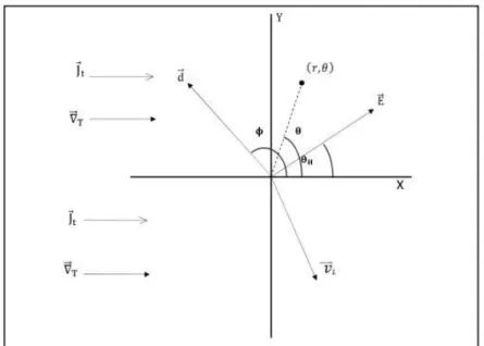
In order to derive the vortex dynamics equation, it is neces-sary to introduce a coordinate system. In this sense, as much the applied temperature gradient as the transport current are oriented in x direction. The magnetic field is directed along the z-axis. The vortex velocity vector and the displacement vector~dform anglesθH andφwith the x axis respectively. The geometry of the problem is pictured in Figure 1.
From Figure 1 we have:
~Jt=Jt[cosθeˆr−sinθeˆθ], (27)
~∇T =∇T[cosθeˆr−sinθeˆθ], (28)
~vL=vL[sin(θ−θH)eˆr+cos(θ−θH)eˆθ], (29)
~
d=d[cos(θ−φ)eˆr+sin(θ−φ)eˆθ]. (30) The differential equation for the scalar potentialPacquires the following form:
σ(xxn)
k2 ∇ 2P
−γ1P f02=
[γ2f0 d f0
dr − σ(xyn)
k dh0
dr ]vLsin(θ−θH) + b(xxn)
k2 ∇ 2T
cosθ. (31)
In the above equation~h0=~∇×Q~0. It is possible to determine the form of the solution to the equation (31) considering the limit r→0, thenχ→θ. Therefore, from the equation (2) we haveP≈ −∂χ∂t ≈~vL.~∇θ=1reˆθ.
In general way, the solution to the non homogenous differen-tial equation (31) takes the form:
P(~r) =vLp1(~r)cos(θ−θH) +vLp2(~r)sin(θ−θH) +p3(~r), (32) wherep1is the solution to the homogenous equation (31),p2 andp3are particular solutions to the nonhomogenous equa-tion. From the previous expression, we have that,p1,p2and p3satisfy the differential equations:
σ(xxn) κ2 ∇
2p1−γ
1f02p1=0, (33)
σ(xxn) κ2 ∇
2p
2−γ1f02p2=γ2f0 d f0
dr − σ(xyn)
κ dh0
FIG. 1: Geometry of the system
σ(xxn) κ2 ∇
2p
3−γ1f02p3= b(xxn)
κ2 ∇
2Tcosθ. (35)
As~∇T acts on normal electrons for small values ofr(r→0) then f02→0 and for high values ofrsuperelectrons do not feel the presence of the temperature gradient, reason why in the equation (35) the second term of the left side can be neglected, having the solution (32) the form:
P(~r) = ~vLp1(~r)cos(θ−θH) +
+~vLp2(~r)sin(θ−θH)−ε|~∇T|rcosθ, (36) where the parameterε=b(xxn)
σ(xxn)
was introduced.
3. VORTEX DYNAMICS EQUATION
The solvability condition can be evaluated solving the equation (26). The surface integral can be expressed in terms
of the applied transport current at the borders, where
~
J1s(r=∞,θ) =~Jt, ~Jd.eˆr=dsin (θ−φ)
κr2 ,
χ1=κJtrcosθ,χd≡~d.~∇θ=dsin (θ−φ)
r , (37)
so that the first integral to evaluate is the only one in the left side of the equation (26), where we use the formulae for the transport current~Jt andχdin cylindrical coordinates shown in the equations (27) and the trigonometric equality sin(θ−φ) =sinθcosφ−cosθsinφ,
1 κ
Z
d~S·[~J1sχd−~Jdχ1] = 1 κ
Z
(rdθˆer)·(J~tχd)− 1 κ
Z
(rdθeˆr)·(~Jdχ1) = 1
κ
Z
(rdθˆer)·(J~tχd) =− 2 κJtd
Z 2π
0 cosθsin(θ−φ)
dθ=−2πκ(~Jt×eˆz)·d~. (38)
The following term to solve is the first integral of the right side of the equation (26), which with the aid of the relation
(36) is written as follows
Z
d2rP f0fd =γ2
Z ∞
0
Z 2π
0
drdθ{vLp1cos(θ−θH)+
Developing the product f0fdand using the expression for ~
d, given in equation (30), we have γ2
Z
d2rP f0fd =−γ2π
2 (~vL×eˆz)·d~
Z ∞
0 (
f02)′r p1dr− γ2π
2 ~vL·d~
Z ∞
0 (
f02)′r p2dr
−πγ2ε~∇T·d~
Z ∞
0 (
f02)′r2dr. (40) Solving the second integral in the right side of the equation (26), one must account the relations (12) and (15), obtaining
γ1
Z
d2r fvfd=γ1
Z
d2r(~vL·~∇f0)(d~·~∇f0)
=−π~vL·d~γ1
Z ∞
0 (
f0′)2rdr, (41)
where we have introduced the projections for~vLandd~given by the equations (29) and (30) respectively. Now to calculate the third term of the equation (26), we expand ρn(~r) in a Taylor’s series around the vortex centre
ρn(~r) =ρn(0) +~r·~∇ρn(0) +(~r·~∇)
2
2 ρn(0) +. . .
Accounting that, the position vector in cylindrical coordi-nates has the form~r=r[sin(θ−θH)eˆr+cos(θ−θH)eˆθ]and
taking the scalar product, the functionρn(~r)can be written in the following way
ρn(~r) =ρn(0) +rsin(θ−θH) ∂ ∂rρn(0)
+cos(θ−θH) ∂
∂θρn(0)+ r∂∂rρn(0)
2 −
rsin(θ−θH)cos(θ−θH)
2 . (42)
Taking the gradient of the function (42) in the limitr→0, we obtain:
~∇ρn(~r) =∂ρn(0)
∂r (eˆr+eˆθ), (43) where we have considered thatρn(~r)also grows in the−eˆr direction. Replacing the equation (43) in the solvability con-dition, the third term of this expression acquires the form:
1 κ
Z
d2rχd~vn·~∇ρn(rˆ) = π
2κ[(~vn×eˆz)·d~]ρn(0)+ π
κ[~vn·d~]ρn(0). (44) Equally, the term associated to~vLin the solvability condition is obtained as follows:
1 κ
Z
d2rχd~vL·~∇ρn(rˆ) =−
dvn
2 ×
Z 2π
0 sin(
θ−θH)[sin(θ−θH) +cos(θ−θH)]dθ
Z ∞
0 ∂
∂rρn(0)dr
=
π
2κ[~vL×eˆz·~d]ρn(0) + π
κ[~vL·d~]ρn(0). (45)
Finally, the fourth integral in equation (26) is solved using the relations (37) and (29):
1 κ
Z
d2rχd~vL·~∇ρs(rˆ) = −dvκL
Z 2π
0
sin(θ−φ)sin(θ−θH)dθ
Z ∞
0 ∂ρs
∂r dr
=−πρs[(~vL×eˆz)·d~]. (46) The equation of motion is obtained from the solvability condition when we replace the results obtained in equations (38), (40), (41), (44), (45) and (46). In a compact form the equation of motion can be written:
ρs[(~vs−~vL)×~κ˜] =D(~vL−~vn) +D′[eˆz×(~vL−~vn)] +d~vL +d′(eˆz×~vL) +Sv~∇T. (47) In the above equation,~κ˜is the quantum of circulation and we have taken account that~Jt=~Js/2 and~Js=ρs~vs. In addition
we have defined the coefficients
D=−κρ˜ n, D′=κρ˜ n, (48)
d=κκγ˜ 1
Z ∞
0
(f ′0)2r2dr−κκ˜γ2 2
Z ∞
0
p2(f02)′r2dr, (49)
d′=κκ˜γ2 2
Z ∞
0
p1(f02)′r2dr, (50)
Sv=2γ2ηκκ˜
Z ∞
0
(f02)′r2dr, (51)
ρn=ρn(0). (52)
phenomenological way [11]. In the present development this equation is obtained in a natural way from the time depen-dent Ginzburg - Landau equation. The term of the left side of equation (47) represents the Magnus force, which is con-nected to the momentum transfer between the vortex and the the superfluid. The forces proportional toDandD′are due to dispersion of quasi particles by the vortices, presenting a momentum transfer between the vortex moving with velocity ~vLand the normal fluid moving with velocity~vn. The trans-verse component of this interaction is the Iordanskii force. The forces proportional todandd′, according to Kopnin and Kravtsov [15], are due to vortex relaxation processes associ-ated to the vortex interaction impurities which are at rest in the lattice. The transverse component of this interaction is the Kopnin-Kravtsov force. The force proportional to~∇T is connected to the vortex thermal flow with a transport entropy Sv. If a moving vortex transports entropy, it experiences a force in a temperature gradient. The excistence of this force is well known from experimental data [12,13,14].
4. CALCULATION OF THE COEFFICIENTSd,d′ANDSv
In this section we will determine the explicit form for the coefficients, which are connected to relaxation processes in the vortex dispersion so as the entropySvdue to the thermal motion. In general, when the Ginzburg-Landau equation is solved, one take some conjectures about the profile of the order parameter inside the vortex. An approach of the vari-ation of dimensionless order parameter, which we will use, was proposed by Brandt [16]. In the present analysis we will find solutions in the limitr→0 where the order parameter has the form
f02
2 ≃1−e −r2
2ξ20 ≃ r
2
2ξ2 0
(53)
Whereξ0is the coherence length. Replacing the equation (53) in the equation (33), the following equation in cylindri-cal coordinates is obtained:
∂2p 1 ∂r2 +
1 r
∂p1 ∂r −Rr
2p
1=0 (54)
where the parameterR=κ2γ 1ξ20σ
(n)
xx was introduced. The differential equation (54) has a solution in power’s series given by the expession p1(r) =Σ∞n=0anrn+q, whereq=−1. The asymptotic solution to the equation (54) must consider that:
P = Φ+∂χ ∂t =~v·
~∇χcos(θ−θH) =v~∇χcos(θ−θH)
≈ 1rvcos(θ−θH). (55)
From the previous analysisp1(r)≈1/rin the limitr→0. In the same way for the magnetic vector we haveQ0(r)≈
−1
κ∇χ≈ −kr1. But on the other hand,Q0satisfies the rela-tionh0=~∇×Q~0, whereQ0(r) =12h0(0)rwhich determines the solutionQ0(r) =−kr1+
1
2h0(0)r, whereh0(0)is the mag-netic field in the vortex center. In this sense, accounting the
relation (55) in the limit r→0, then we havea1 = 0 and therefore
p1(r)≈ 1
r. (56)
In order to determinep2(r)in the same way that forp1(r), we look to the solution of the equation (32), in power series and doing all the previous procedure one obtain
p1(r)≈ 1
r−p2cr. (57)
Now we are able to determine coefficientsd ,d′ andSv. Replacing the expressions (56) and (57) in the equations (49), (50) and (51) in the limitr→0:
d=κκγ˜ 1
Z ∞
0 (
f ′0)2rdr+γ2 2
Z ∞
0
p2(f02)′rdr=κ(γ2−γ1)ρs, (58)
d′=−κκ˜γ2 2
Z ∞
0
p1(f02)′rdr=−κγ2ρs, (59)
Sv=2 ˜κκγ2η
Z ∞
0 (
f02)′r2dr=κκγ˜ 2η
√
2πξo. (60)
From the above equations we observe that the parameter d, which is associated to the interaction with impurities, has a double nature, the first one is connected to the Bardeen-Stephen mechanism of dissipation, whereas the second con-tribution is due to variations in the local charge density in the vortex interaction with impurities. The same effect occurs in the obtaining of the coefficientd′. Equally it is important to notice that the transport entropy posses a direct relation to re-laxation processes due to the condensation and Coopers pair breaking by different pairing potentials via vortex motion as it is shown in equation (60).
5. SUMMARY
Acknowledgements
The Authors would like to thank the financial support granted by the Universidad del Atl´antico.
[1] J.M. Harris, N.P. Ong and Y.F. Yan, Phys. Rev. Lett.71, 1455 (1993).
[2] S.J.Hagen et al., Phys. Rev. B47, 1064 (1993).
[3] J. Bardeen and M.J. Stephen, Phys. Rev.140, A1197 (1965). [4] P. Nizierese and W.F. Vinen, Philos. Mag.14, 667 (1966). [5] A.T. Dorsey, Phys. Rev. B46, 8376 (1992).
[6] L.P. Gorkov and N.B. Kopnin, Sov. Phys. Usp.18, 496 (1975). [7] P. Ao and Thouless, Phys. Rev. Lett.70, 2158 (1993) [8] P. Ao and Q Niu, Phys. Rev. Lett.76, 3758 (1996)
[9] G. Blatter, V.G. Geshkenbein and N.B. Kopnin, Phys. Rev B
59, 14663 (1999)
[10] N.B. Kopnin, Rep. Prog. Phys.65, 1633 (2002)
[11] A. Freimuth and M. Zittartz, Phys. Rev. Lett.84, 4978 (2000). [12] R.P. Huebner, Supercond. Sci. Technol.8, 189 (1995). [13] T.T.M. Palstra et al., Phys. Rev Lett.64, 3090 (1990). [14] M. Zeh et al., Phys. Rev. Lett.64, 3195 (1990).