Use of direct and iterative solvers for estimation of SNP effects in genome-wide selection

Use of direct and iterative solvers for estimation of SNP effects in

genome-wide selection

Eduardo da Cruz Gouveia Pimentel

_{, Mehdi Sargolzaei}

_{, Henner Simianer}

_{, Flávio Schramm Schenkel}

_,

Zengting Liu

_{, Luiz Alberto Fries}

_{and Sandra Aidar de Queiroz}

1

_{Animal Breeding and Genetics Group, Department of Animal Science, Georg-August-University}

of Göttingen, Göttingen, Germany.

2

_{Departamento de Zootecnia, Faculdade de Ciências Agrárias e Veterinárias,}

Universidade Estadual Paulista ‘Júlio de Mesquita Filho’, Jaboticabal, SP, Brazil.

3

Department of Animal and Poultry Science, Centre for Genetic Improvement of Livestock,

University of Guelph, Guelph, ON, Canada.

4

_{Vereinigte Informationssysteme Tierhaltung w.V., Verden / Aller, Germany.}

GenSys Consultores Associados S/S Ltda., Porto Alegre, RS, Brazil.

Abstract

The aim of this study was to compare iterative and direct solvers for estimation of marker effects in genomic selec-tion. One iterative and two direct methods were used: Gauss-Seidel with Residual Update, Cholesky Decomposition and Gentleman-Givens rotations. For resembling different scenarios with respect to number of markers and of geno-typed animals, a simulated data set divided into 25 subsets was used. Number of markers ranged from 1,200 to 5,925 and number of animals ranged from 1,200 to 5,865. Methods were also applied to real data comprising 3081 individuals genotyped for 45181 SNPs. Results from simulated data showed that the iterative solver was substan-tially faster than direct methods for larger numbers of markers. Use of a direct solver may allow for computing (co)variances of SNP effects. When applied to real data, performance of the iterative method varied substantially, depending on the level of ill-conditioning of the coefficient matrix. From results with real data, Gentleman-Givens ro-tations would be the method of choice in this particular application as it provided an exact solution within a fairly rea-sonable time frame (less than two hours). It would indeed be the preferred method whenever computer resources allow its use.

Key words:breeding value, genomic selection, mixed model equations, numerical method. Received: February 27, 2009; Accepted: November 18, 2009.

Introduction

Most applications in animal breeding involve the so-lution of systems of equations with very large numbers of unknowns. For instance, with multiple or single trait animal models or random regression test-day models the number of parameters increases as a function of the number of ani-mals being evaluated, which are not so rarely in the hun-dreds of thousands or above. The coefficient matrices that arise from these kinds of problems are too large to be stored in high speed memory. For this reason, iterative solvers, both on data or on the mixed model equations, have gained high popularity and are widely employed in genetic evalua-tion of livestock. When an iterative algorithm is applied for

the solution of a linear system, one cannot obtain the ele-ments of the inverse of the coefficient matrix. Therefore, prediction error variances and standard errors of estimates have to be calculated in an indirect way and are conse-quently approximated values.

Recent advances in molecular genetic techniques have led to the availability of information on a large num-ber of sequence variations across the genome. This new source of information has launched a series of studies (e.g., Meuwissenet al., 2001; Xu, 2003) attempting to associate such sequence variations with phenotypic variation in com-plex traits. If the number of identified variations is large enough that it covers the entire genome one could assume that most of the quantitative trait loci (QTL) associated with a given trait will be in linkage disequilibrium with at least some of these markers. Genome assisted breeding val-ues (GEBV) could then be calculated by estimating the ef-fects of QTL associated with the markers, or alternatively www.sbg.org.br

Send correspondence to Eduardo da Cruz Gouveia Pimentel. Ani-mal Breeding and Genetics Group, Department of AniAni-mal Science, Georg-August-University of Göttingen, Albrecht-Thaer-Weg 3, 37075 Göttingen, Germany. E-mail: epiment@gwdg.de.

the effects of the markers themselves, on the traits of inter-est and taking the summation of these effects across the whole genome. High-density panels for genotyping thou-sands of single nucleotide polymorphisms (SNP) are now commercially available and their costs are likely to de-crease over time, which would make genome-wide selec-tion an affordable procedure in the near future (Schaeffer, 2006). The number of unknowns in the models considered for the estimation of SNP effect on total genetic merit of in-dividuals is a function of the number of genotyped SNP, which may be constant over time. A constant number of un-knowns and the increasing rate of advances in computer hardware could make the use of a direct solver an interest-ing option, as that would make it possible to obtain the elements of the inverse of the coefficient matrix for calcu-lating standard errors of estimates.

This research compares the application of iterative and direct solvers for the estimation of SNP effects with po-tential use on genomic selection. Possible computational advantages and disadvantages of the methods were investi-gated.

Material and Methods

Simulated data

A simulated data set prepared for the XII QTL-MAS Workshop, held in Uppsala, Sweden, in May 2008, was used. Data consisted of phenotypes, breeding values and genotypes for 6,000 SNP on 5,865 animals. Markers were evenly distributed on six chromosomes of 100 cM each. Details about the simulation procedures can be found in Lundet al.(2009).

From the 6,000 markers, 75 had the same genotype shared by all animals and were then discarded from the analyses. Twenty five subsets were extracted from the data set, resembling scenarios that differed in the number of evenly spaced markers (1,200, 2,400, 3,600, 4,800 and 5,925) and in the number of genotyped animals (1,200, 2,400, 3,600, 4,800 and 5,865).

Real data

Relative performances of the compared numerical methods were also investigated with their application to real data. A set of 3081 Holstein-Friesian sires genotyped for the Illumina BovineSNP50 BeadChip was used. Fol-lowing usual data quality control procedures, markers with a call rate (i.e., successfully assigned genotype) lower than 90% or minor allele frequency lower than 1% were ex-cluded from the initial set. After filtering, 45,181 markers were kept in the analyses. The response variable used was the estimated breeding value for milk yield.

Equations to solve

A multiple linear regression model (Xu, 2003) was employed to estimate SNP effects on breeding values. The model equation is described below:

y_i x b_{ij j} e_i

j p

= + +

=

å

1

(1)

whereyiis the breeding value of theithanimal;mis an

over-all mean;xijis the coefficient for thejthSNP genotype of the

ithanimal;bjis the slope on thejthSNP genotype;pis the

number of genotyped SNP;eiis a random error.

Coefficientsxijwere set to -1 for genotype A1A1, 0 for genotype A1A2and +1 for genotype A2A2. Regression coef-ficients can be obtained by the solution of the following set of mixed model equations:

i i i

i

m i

t t

t t

t

t

X

X X X b

y X y

+ é

ë

ê ù

û úé

ë

ê ù

û ú =é

ë

ê ù

û ú

F (2)

whereiis a vector of ones, of order equal to the number of genotyped individuals;Fis a square matrix of orderp.

Different statistical models can be defined by alter-nate ways of setting up the matrixF. For the sake of sim-plicity, and as the purpose of this investigation was to compare numerical rather than statistical methods, the ma-trixFused in the application to the simulated data was as-sumed to be an identity matrix.

In the application to the real data, a different proce-dure was conducted in order to resemble a more realistic scenario. The matrixFused was an identity matrix times a ratio of variances, as in the ‘BLUP’ method by Meuwissen

et al.(2001). Furthermore, two alternate forms of ‘BLUP’ analysis were performed: one in which the set of equations to solve and matrixFwere as previously described and an-other in which each observation was weighted by the effec-tive number of daughter contributions, a measure of the reliability of the corresponding estimated breeding value, which represents a procedure more likely to be used in practice. The second set of equations was of the form:

i i i

i

m i

t t

t t

t

t

W WX

X W X WX b

Wy X Wy

+ é

ë

ê ù

û úé

ë

ê ù

û ú =é

ë

ê ù

û ú F

whereWwas a diagonal matrix withwiielement equal to

the effective number of daughter contributions (Fikse and Banos, 2001) of sirei.

Numerical methods

it-eration. A thorough explanation of the method including the pseudo-code in Fortran 95 (which was used here) is pro-vided by Legarra and Misztal (2008) in a study of possible computational methods for use in genome-wide selection. The convergence criterion employed here was the relative difference between two consecutive solutions (Lidaueret al., 1999) and the stopping point was defined when this dif-ference was lower than 10E-14.

One of the direct methods considered was Cholesky Decomposition (CHD), which was also included in the study by Legarra and Misztal (2008). Briefly, it consists in a factorization of a positive-definite coefficient matrix into the product LLt_{where L is a lower triangular matrix.} There-fore the application of the method involves setting up the mixed model equations, factorizing the left hand side and solving two triangular systems.

The other direct method employed in this study was a row-wise algorithm for orthogonal (QR) decomposition, namely Givens planar rotations (Givens, 1954). According to Baiet al.(2001), orthogonal factorization is strongly ro-bust and numerically stable. The standard form of Givens rotations requires a square root operation per rotation and four multiplications for each pair of off-diagonal elements in the pivot (r) and working (x) rows:

c s s c r r x x r r x c r k k k k -é ë ê ù û úé ë ê ù û

ú =é¢ _¢¢

ë ê ù û ú = 1 1 1 1 0 K K K K r x s x r x ri cri sxi xi sri cxi

1 2 1 2 1 1 2 1 2 + = + ¢ = + ¢ = - + ; ; (3)

Following the rationale underlying the square root free version of Gram-Schmidt orthogonalization, Gentle-man (1973) proposed a modification of the procedure in order to save the square root operation in (3). The modifica-tion consists in finding not the triangular matrix R (from the QR decomposition) itself, but rather a diagonal matrix D and a unit upper triangular matrixRsuch that:

R D R= 0 5. (4)

The modified algorithm thus rotates a row of the productD R0 5. with a scaled row of X:

0 0

0 0

K K K

K K K

d d r

x x

k

i k

d d

and the transformed rows can be written:

0 0

0 0 0

K K K

K K K

¢ ¢ ¢

¢ ¢

d d r

x k k d where ¢ = + ¢ = ¢ = ¢ = ¢ ¢ = - ¢ = +

d d x d d

c d d s x d

x x x r r cr

i

i

k k i k k k

d d d

d 2

/

/ /

s x_k

(5)

Besides avoiding the square root operation in (3), the updating formulae in (5) also take only three multiplica-tions for each pair of elements involved in the rotation. Actually, with a slight modification, an extra multiplication could still be saved, but it would compromise stability (Bai

et al., 2001). Here an algorithm using the formulae in (5) presented by Gentleman (1974) was applied and referred to as Gentleman-Givens (GG) algorithm.

For all the scenarios simulated analyses were run us-ing the three numerical methods, and computational re-quirements in terms of time and memory were measured. All the analyses of the simulated data were run on a 2.0 GHz Intel® E4400 processor in a PC with 2.0 Gb of RAM. The analyses with the real data required a larger amount of memory and were therefore run on an SGI Altix 4700 system in which each computer blade had a Dual-Core Itanium2 Processor (1.6 GHz clock speed, 533 MHz frontside bus, 16 Mb 3 level cache) with at least 8 Gb of RAM.

Results

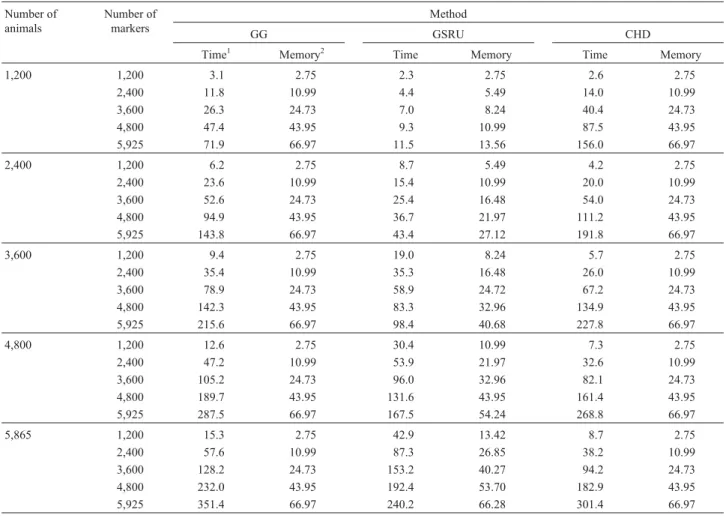
Table 1 presents total processing times and memory requirements for methods GG, GSRU and CHD for the dif-ferent numbers of animals and markers considered in the simulated data. In all scenarios identical solutions were ob-tained by the three methods. The iterative method did not have any problem related to convergence and the defined convergence criterion with stopping point at 10E-14 was effectively achieved. The average number of iterations was 582±50.

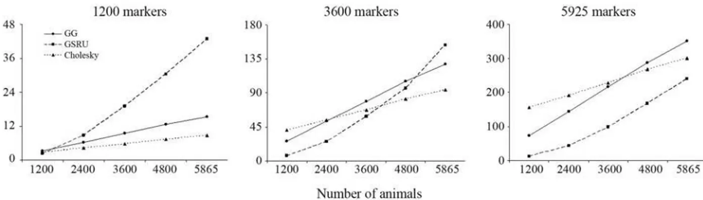
In the situation with the lowest number of markers GSRU was the fastest when the number of animals was also the lowest. As the number of animals increased, processing time with GSRU increased at a higher rate than with GG and CHD. Moreover, as the number of markers increases, the advantage of GSRU over the direct methods persists over an increasing number of animals, up to the point when it is the fastest method for any number of animals. How-ever, in terms of computing time, it is expected that the di-rect methods finally outperform GSRU when the number of animals becomes very large. This trend is illustrated in Fig-ures 1 and 2.

597, 6,235 and 41,011 s for GSRU, GG and CHD respec-tively. The solutions from GSRU converged (relative dif-ference between two consecutive solutions lower than 10E-14) after 3,513 iterations.

With the weighted version of the analyses the pro-cessing time required by the direct methods did not

change: 6,228 and 40,856 s for GG and CHD respec-tively. However, although weighting the observations did not cause any exact linear dependency, it turned the coefficient matrix to be ill-conditioned and considerably slowed down the rate of convergence with GSRU. The log10 of relative differences between consecutive

solu-Table 1- Computational requirements for solving the equations using Gentleman-Givens (GG), Gauss-Seidel with Residual Update (GSRU) and Cholesky decomposition (CHD), for the different numbers of animals and markers contemplated in the simulated data set.

Number of animals

Number of markers

Method

GG GSRU CHD

Time1 _Memory2 _{Time Memory Time Memory}

1,200 1,200 3.1 2.75 2.3 2.75 2.6 2.75

2,400 11.8 10.99 4.4 5.49 14.0 10.99

3,600 26.3 24.73 7.0 8.24 40.4 24.73

4,800 47.4 43.95 9.3 10.99 87.5 43.95

5,925 71.9 66.97 11.5 13.56 156.0 66.97

2,400 1,200 6.2 2.75 8.7 5.49 4.2 2.75

2,400 23.6 10.99 15.4 10.99 20.0 10.99

3,600 52.6 24.73 25.4 16.48 54.0 24.73

4,800 94.9 43.95 36.7 21.97 111.2 43.95

5,925 143.8 66.97 43.4 27.12 191.8 66.97

3,600 1,200 9.4 2.75 19.0 8.24 5.7 2.75

2,400 35.4 10.99 35.3 16.48 26.0 10.99

3,600 78.9 24.73 58.9 24.72 67.2 24.73

4,800 142.3 43.95 83.3 32.96 134.9 43.95

5,925 215.6 66.97 98.4 40.68 227.8 66.97

4,800 1,200 12.6 2.75 30.4 10.99 7.3 2.75

2,400 47.2 10.99 53.9 21.97 32.6 10.99

3,600 105.2 24.73 96.0 32.96 82.1 24.73

4,800 189.7 43.95 131.6 43.95 161.4 43.95

5,925 287.5 66.97 167.5 54.24 268.8 66.97

5,865 1,200 15.3 2.75 42.9 13.42 8.7 2.75

2,400 57.6 10.99 87.3 26.85 38.2 10.99

3,600 128.2 24.73 153.2 40.27 94.2 24.73

4,800 232.0 43.95 192.4 53.70 182.9 43.95

5,925 351.4 66.97 240.2 66.28 301.4 66.97

1_{in seconds.}

2_{in Megabytes.}

tions across iterations are shown in Figure 3. A less strin-gent stopping point (10E-12) had to be set in order to obtain solutions within a reasonable time frame. This threshold was achieved after 150,850 iterations. Solu-tions obtained at this point were almost the same as the ones obtained with the direct methods. Correlation was greater than 0.999 and mean and maximum absolute dif-ference between SNP effect estimates were 0.07 and 0.72 respectively. The time required to achieve this level of convergence was 24,759 s. An even less stringent stop-ping point (10E-10) was also tried and solutions con-verged at this level in 1989 s after 12,073 iterations, but the mean and maximum absolute difference between es-timates increased to 0.18 and 1.78 respectively. As pointed out by Legarra and Misztal (2008) it may be pos-sible to speed up the rate of convergence by the use of a relaxation factor, but this factor would have to be deter-mined empirically. Such an approach was not conducted here in order to keep the different performances of the al-gorithms comparable.

Discussion

Results from the simulated data illustrate the relative performance of the different numerical methods and their deviations from what would be expected from just a com-plexity analysis of the algorithms. With fewer animals GSRU was the fastest method regardless the number of markers whilst processing time sharply increased when using a direct solver, more pronouncedly with CHD. Legarra and Misztal (2008) compared several numerical methods to be considered in SNP effect estimation using a data set with ~11,000 SNPs and ~2,000 animals. They fit-ted a model with additive and dominance effects so the to-tal number of unknowns was ~22,000. In their study, the processing times with GSRU and CHD were 1.5 and 136 min, respectively.

As it can be seen from Table 1, the main advantage of GSRU over GG and CHD is the low memory requirement, which makes it suitable for situations when the number of parameters is very large. The memory requirement of GSRU was a linear function of the number of parameters while memory required by GG and CHD grew quadra-tically with the number of parameters.

Based on the numbers of arithmetic operations in-volved in each procedure one would expect that GSRU would be faster than both CHD and GG for increasing num-ber of markers, unless a very large numnum-ber of iterations were necessary. The number of operations involved in CHD is np2/2 for setting up the mixed model equations and (1/3)p3for the factorization, where p is the number of un-knowns and n the number of observations. The QR decom-position via GG requires 2np2 operations. On the other hand, in GSRU the number of operations is 3np times the number of iterations.

Since GG implies the application of a sequence of planar rotations on the rows of the data matrix, setting up the normal equations is not necessary. One then has to add some pseudo-observations to the system in a way that is equivalent to setting up the equations in (2). The data ma-trix to be factorized becomes:

Figure 2- Relative performance of the methods for the lowest, intermediate and the largest number of markers in the simulated data set.

i X y

~ . ~

0 F0 5 0

ì í î

ü ý

þ (6)

For the diagonal variance structure of the random ef-fect, the above redefinition is fairly straightforward and the elements of the pseudo-observations matrix are easy to compute.

Augmenting the data matrix by a set of p pseudo-observations would dramatically increase the amount of arithmetics needed for decomposition, but this can be avoided with the following procedure. The order by which the rows of data are rotated does not affect the factorization into the product QR. Therefore, the pseudo-observations can be rotated first. Since they consist of just a diagonal ma-trix this can be achieved by simply initializing this diagonal as the initial diagonal of R (instead of a vector of zeros), which avoids the extra p2transformations implied by the augmentation. This strategy was applied here and made the addition of the pseudo-observations as (almost) costless as the addition of matrixFto the random part of the MME in (2). It explains in part why GG was still faster than CHD in situations with larger numbers of markers and fewer ani-mals, as it would be expected based on the number of oper-ations in the case of non-augmented matrices (e.g., fixed regression).

Legarra and Misztal (2008) pointed out that in large SNP data applications setting up the MME incurs in a large amount of non-zeros on the left hand side of the equations, which makes the system fairly dense. Therefore, with CHD it is not possible to take any advantage of the sparsity result-ing from the form of parameterization applied here. On the other hand, the use of GG makes it possible to explore spar-sity (not in terms of storage but in terms of savings in arith-metic operations). Since the MME are not explicitly set up, all the zeros corresponding to heterozygous genotypes in the data matrix are preserved, and this can be readily ex-ploited by simply skipping the transformation. An example evidence of these savings can be illustrated by the compari-son between the processing times required by GG and GSRU in the scenario with the largest number of animals and markers. Based on the number of operations alone (2np2versus 3np times 950 iterations), one would expect that the difference in processing time between GG and GSRU would be almost seven times the observed one. The difference in processing time between GG and CHD when applied to real data was also much larger than would be ex-pected from the number of operations only. It also reflects the impact of these savings in the relative performance of the algorithms.

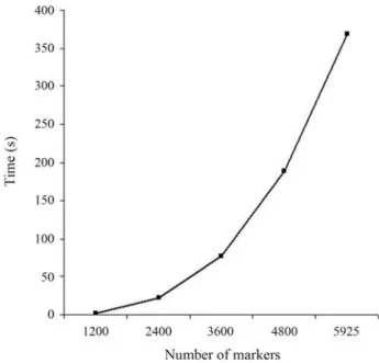
The use of a direct solver can allow for calculations that are not possible with an iterative approach. For in-stance, a property of GG is that the upper triangular R ob-tained by QR factorization of a matrix A is equivalent to the Cholesky factor of the coefficient matrix AtA from the nor-mal equations. Given that property, it is possible to

calcu-late the elements of (AtA)-1 directly from R without the need for explicitly setting up the normal equations. Since AtA = RtR then (AtA)-1= R-1R-t. To simplify the notation, let’s call (AtA)-1= M with columns m1, m2, mn, so that RM = R-t. Then, since R is upper triangular and R-tis lower triangular, and noticing that the ithdiagonal of R-tis the re-ciprocal of the ithdiagonal of R, it is possible to compute the elements of columns mn to m1 from bottom to top, one col-umn at a time. An efficient algorithm for computing the di-agonals of the inverse can be found in Lawson and Hanson (1974). Figure 4 presents the time required for calculating exact standard errors of estimates from the simulated data using their algorithm for obtaining the diagonals of the in-verse. It can be seen that the increase in time is approxi-mately exponential and therefore this procedure is feasible only in the case of applications with limited number of pa-rameters. For instance, with the real data used in this study the calculation was not even attempted. Because of over-parameterization problems in the genomic selection con-text, efforts are underway to reduce the dimensionality of the problem (e.g., Longet al., 2007; Habieret al., 2009). In the case of pre-selection of a subset of most relevant mark-ers (e.g., tag SNP) a direct solver could be used for comput-ing (co)variances of SNP effects. In this case, method GG as implemented here could be an interesting alternative to CHD for a few thousand genotyped animals. If a larger panel, say 50 k, is still preferred and one is interested in computing (co)variances, this would be possible by block-ing the SNPs of interest. For instance, one would likely be interested in investigating covariances among marker ef-fects within some segments of the genome (e.g., chromo-some-wise). Reordering the SNPs of interest to be in the

bottom part of R, one can easily compute the inverse of the last portion of the upper-triangular matrix. In the 50 k panel, the largest number of markers within a chromosome was less than 3000, so the computation would take just a few minutes, as shown in Figure 4.

As discussed earlier, with increasing number of markers the difference in speed between the iterative and direct solvers used here tends to become more relevant. Nevertheless, processing time is not the only issue to be ad-dressed in the comparison. In fact, since the matrices to be handled in these applications are dense, memory require-ments are major factors in the decision on which method to use. In the implementation of GSRU the data matrix was kept in high speed memory during the whole execution, be-cause the size of problem tested here (both with the simu-lated and real data) allowed for it. For larger problems though the program can be easily adapted to read it from hard disk, keeping memory requirements at a very low level. On the other hand, the direct solvers required the allo-cation of p*(p+1)/2 positions of memory in a half-storage structure. For five or ten thousand markers this would mean approximately 190 Mb (in single precision) at most, which is not such a high demand even for current personal com-puters. The memory requirement increases quadratically with the number of markers. With the application to the real data for example, moving to ~45,000 markers took about 3.8 Gb and required the use of a more powerful machine. Therefore, memory space and computer resources avail-ability are usually the main issue determining the applica-bility of direct methods.

The relative performance of the solvers may differ in different scenarios, as shown with the simulated data in Figures 1 and 2 and with the real data from the results of the weighted and unweighted analyses. It is therefore difficult to give a general recommendation on which method to use. From the results of the analysis with the real data in the weighted case, GG would be the method of choice in this particular application as it provided an exact solution within a fairly reasonable time frame (less than two hours). It would indeed be the preferred method whenever com-puter resources allow its use. If the number of markers to be used in the estimation of genomic breeding values were in the hundreds of thousands, then GSRU would definitely be the method of choice, if not the only practically feasible due to memory requirements and the current status of comput-ing power. One would then have to experimentally define a relaxation factor in order to speed up convergence rate. For the current dimension of the SNP effect estimation problem in a farm animal context (i.e., ~50 k) the direct methods were still applicable in practice. It is clear that computer and genotyping technologies are both developing with an outstanding rate of progress so it is reasonable to anticipate that in many future situations a direct solver may be still ap-plicable.

Acknowledgments

This study is part of the project FUGATO-plus GenoTrack and was financially supported by the German Ministry of Education and Research, BMBF, the Förder-verein Biotechnologieforschung e.V. (FBF), Bonn, and Lohmann Tierzucht GmbH, Cuxhaven. The first author was sponsored by a scholarship from Coordenação de Aperfeiçoamento de Pessoal de Nível Superior (CAPES, Brazil).

References

Bai Z-Z, Duff IS and Wathen AJ (2001) A class of incomplete or-thogonal factorization methods. I: Methods and theories. BIT 41:53-70.

Fikse WF and Banos G (2001) Weighting factors of sire daughter information in international genetic evaluations. J Dairy Sci 84:1759-1767.

Gentleman WM (1973) Least squares computations by Givens transformations without square roots. J Inst Maths Applics 12:329-336.

Gentleman WM (1974) Algorithm AS 75: Basic procedures for large, sparse or weighted linear least problems. Appl Stat 23:448-454.

Givens W (1954) Numerical Computation of the Characteristic Values of a Real Symmetric Matrix. Oak Ridge National Laboratory Report, Oak Ridge, ORNL 1574.

Habier D, Fernando RL and Dekkers JCM (2009) Genomic selec-tion using low-density marker panels. Genetics 182:343-353.

Janss L and de Jong G (1999) MCMC based estimation of vari-ance components in a very large dairy cattle data set. Interbull Bull 20:62-67.

Lawson CL and Hanson RJ (1974) Solving Least Squares Prob-lems. 1st edition. Prentice-Hall, New Jersey, 340 pp. Legarra A and Misztal I (2008) Computing strategies in

ge-nome-wide selection. J Dairy Sci 91:360-366.

Lidauer M, Strandén I, Mäntysaari EA, Pösö J and Kettunen A (1999) Solving large test-day models by iteration on data and preconditioned conjugate gradient. J Dairy Sci 82:2788-2796.

Long N, Gianola D, Rosa GJM, Weigel KA and Avendaño S (2007) Machine learning classification procedure for select-ing SNPs in genomic selection: Application to early mortal-ity in broilers. J Anim Breed Genet 124:377-389.

Lund MS, Sahana G, deKoning D-J and Carlborg Ö (2009) Com-parison of analyses of the QTLMAS XII common dataset. I: Genomic selection. BMC proceedings 3(Suppl 1):S1. Meuwissen THE, Hayes BJ and Goddard ME (2001) Prediction of

total genetic value using genome-wide dense marker maps. Genetics 157:1819-1829.

Schaeffer LR (2006) Strategy for applying genome-wide selec-tion in dairy cattle. J Anim Breed Genet 123:218-223. Xu S (2003) Estimating polygenic effects using markers of the

en-tire genome. Genetics 163:789-801.

Associate Editor: Luciano da Fontoura Costa