André Gil Fernandes de Mendonça
Dissertation presented to obtain the
Ph.D. degree in Biology | Neuroscience
Instituto de Tecnologia Química e Biológica António Xavier | Universidade Nova de Lisboa
Insert here an image
with rounded corners
André Gil Fernandes de Mendonça
Dissertation presented to obtain the
Ph.D. degree in Biology | Neuroscience
Instituto de Tecnologia Química e Biológica António Xavier | Universidade Nova de Lisboa
Oeiras,
December, 2015
The role of reinforcement learning
in perceptual decision-making
The role of reinforcement learning in
perceptual decision-making.
Andr´e Gil Fernandes de Mendonc¸a
A Dissertation Presented to the Faculty of Universidade Nova de Lisboa
in Candidacy for the Degree of Doctor of Philosophy
Zachary F. Mainen
Acknowledgments
{I’m not good with acknowledgments. I always feel that I won’t be able to find the right words for what I mean. Thus, I decided to take the words of others. I love music and dance. Consider this a mashed-up playlist, a medley of lyrics. Some songs remind me of the footnoted people, some are in there just because the lyrics for some reason match a story or a place, sometimes both, sometimes none. So, don’t read too much in-between the lines as sometimes they’re just meant to be silly. Also, I’m always scared that I might have forgotten someone. If I did, I’m sorry. . .}
Everyday when I wake up, I thank the lord I’m Welsh.1 He said, I
locked you in this body, I meant it as a kind of trial. You can use it for a weapon, or to make some woman smile.2 {But, I asked,} who’ll be my role-model, now that my role-model is gone, gone?3
{I was lucky enough to be part of a we} and we’ll never be royals, royals. It don’t run in our blood, that kind of luxe just ain’t for us. We crave a different kind of buzz.4 And they said it changes when the sun
goes down, yeah, they said it changes when the sun goes down.5
{Much, much later}she said it grieves me so to see you in such pain, I wish there was something I could do to make you smile again.6 {Oh! But you did!}
{Looking back, when my despair was too much, not all was lost as you gave me the space and} you came to take us, all things go, all things go, to re-create us.7 And if my parents are crying, then I’ll dig a tunnel from my window to yours, yeah, a tunnel from my window to yours.8 {Truth
1To my sister, Rute
2To my parents, Elisa and Vitoriano
3To my family, specially ´Alvaro, Gabi, Sim˜ao and T´omas 4Toelas. . .
5. . . and toeles, they know whothey are 6To Ana
is}triangles are my favorite shape, three points where two lines meet, toe to toe, back to back.9 {But time is short and I came to realize:} it’s the
final countdown, the final countdown, the final countdown.10 {“I have to finish this...”} and never mind that noise you heard, it’s just the beasts under your bed, in your closet, in your head.11
Sometimes I wonder if the world’s so small, that we can never get away from the sprawl, living in the sprawl.12 ’Cause they know, and so do I, the high road is hard to find, a detour to your new life.13 {I learned that you should} blow steam in the face of the beast - “sky could fall down, wind could cry now. Look at me motherfucker, I smile!”.14 Hang on to the good days, I can lean on my friends, they help me going through hard times.15 And if I made a fool, if I made a fool, if I made a fool, on the road, there’s always this and if I’m sewn into submission I can still come home to this.16
{Because}I feel your whisper across the sea, I keep you with me in my heart, you make it easier when life gets hard.17
Bad mistakes - I’ve made a few. I’ve had my share of sand kicked in my face but I’ve come through.18 But there’s one sound, that no one knows: what does the fox say?19
We are the people that rule the world, a force running in every boy and girl, all rejoicing in the world.20 {And} I try to laugh about it, cover it
9To Alex 10To Eric 11To Gil 12To Patr´ıcia 13To Anna 14To Zaca 15To Rita F´elix
16To Chico, Timon, Nico, Andreia, Sam, Rodrigo 17To Inˆes
all up with lies, I try and laugh about it.21 Ooh, when all I was searching for was me. Keep your head up, keep your heart strong.22 “Bamos l´a
cambada, todos `a molhada que isto ´e futebol total.”23 Some of those that work forces are the same that burn crosses. Uggh! Killing in the name of!24
Lose yourself to dance, lose yourself to dance, lose yourself to dance!25 ’Cause we are the champions, my friends, and we’ll keep on fighting ’til the end. We, are the champions.26
And if I had the choice, yeah, I’d always wanna be there, those were the best days of my life.27
Decisions are made and not bought. But I thought this wouldn’t hurt a lot. I guess not.28
T´ıtulo
O papel da aprendizagem por refor¸co em sistemas de decis˜ao percep-tuais.
Resumo
A acumula¸c˜ao de evidˆencias ´e uma componente importante nas tomadas de decis˜ao perceptuais (perceptual decision-making, PDM) que permite aos organismos mitigar os efeitos de incerteza no ambiente atrav´es da combina¸c˜ao temporal de informa¸c˜ao. Os modelos te´oricos mais simples de acumula¸c˜ao de evidˆencias tˆem sido bem sucedidos a descrever aspectos relacionados ao desempenho em tarefas psicof´ısicas, capturando a inter-dependˆencia entre precis˜ao e tempos de reac¸c˜ao (reaction times, RTs). No entanto, outros aspectos chave deste tipo de modelos permanecem substancialmente amb´ıguos.
Um fen´omeno que ainda n˜ao ´e bem compreendido reside no facto de nem todas as decis˜oes beneficiarem de acumula¸c˜ao de evidˆencia na mesma escala de tempo. Por exemplo, ratos que executam uma tarefa de dis-crimina¸c˜ao auditiva parecem integrar evidˆencia durante mais de um se-gundo. Mas, perante uma tarefa de categoriza¸c˜ao de misturas de odores os benef´ıcios de integrar por mais tempo desaparecem. Uma poss´ıvel ex-plica¸c˜ao ´e a de que os mecanismos de integra¸c˜ao neurais s˜ao espec´ıficos `
Em modelos de acumula¸c˜ao de evidˆencias a principal fonte de in-certeza ´e estocacidade na evidˆencia sensorial. Estas flutua¸c˜oes r´apidas permitem explicar os benef´ıcios de integra¸c˜ao temporal. Outra fonte po-tencialmente importante de incerteza reside nas flutua¸c˜oes na taxa m´edia de acumula¸c˜ao. Tais flutua¸c˜oes correspondem variabilidade no mapea-mento de dados sensoriais numa determinada escolha (tentativa e erro). Esta variabilidade na categoria seria particularmente importante quando o mapeamento de est´ımulo a ac¸c˜ao tˆem que ser aprendidas de novo, como ´e o caso numa tarefa de classifica¸c˜ao de est´ımulos perceptuais.
Neste estudo, este problema foi abordado atrav´es da compara¸c˜ao da inter-dependˆencia entre RT e exactid˜ao em duas tarefas de decis˜ao que eram idˆenticas excepto na natureza dos est´ımulos apresentados. A primeira tarefa consistiu na categoriza¸c˜ao de uma mistura de odores em que a dificuldade foi aumentada ao fazer com que os est´ımulos se situassem mais pr´oximos de uma determinada categoria. A segunda tarefa consistiu na identifica¸c˜ao de odores em que a dificuldade foi aumentada atrav´es da redu¸c˜ao da concentra¸c˜ao total dos odores. Verificou-se que a mudan¸ca de RT durante um determinado intervalo de precis˜ao era diferente entre as duas tarefas. A nossa hip´otese ´e que as flutua¸c˜oes na separa¸c˜ao entre categorias reflectem uma forma de constante de aprendizagem por refor¸co (reinforcement learning, RL). De acordo com RL, as escolhas devem ser reguladas por um mecanismo baseado na expectativa de recompensas. RL ´e uma teoria normativa que postula que os agentes aprendem o valor de diferentes op¸c˜oes de escolha a partir da hist´oria dos resultados obtidos previamente. Se um mecanismo de RL ´e respons´avel pela diferen¸ca ob-servada entre tarefas, ent˜ao os padr˜oes de escolha devem reflectir os erros na previs˜ao de recompensa que s˜ao gerados por diferentes combina¸c˜oes de est´ımulo / escolha / resultado.
Abstract
Evidence accumulation is an important core component of perceptual decision-making that allows organisms to mitigate the effects of environ-mental uncertainty by combining information in time. Simple theoretical models of evidence accumulation have been successful in critical aspects of performance in psychophysical tasks, capturing the inter-dependence be-tween accuracy and reaction time (RT). Yet substantial ambiguity remains concerning key features of this class of models.
One not well-understood phenomenon is that not all kinds of decisions appear to benefit from evidence accumulation over the same time scale. For example, rats performing an auditory discrimination task appear to integrate evidence over one second. But in an odor mixture categorization task rats fail to benefit from longer sampling. A possible explanation is that neural integration mechanisms are specific to a given sensory modal-ity. Different speed-accuracy tradeoffs (SATs) have been proposed as an-other possible explanation for differences seen across similar studies. An alternative proposal is that differences in time arise from different compu-tational requirements. Given that species, modality, task structure have all varied across past studies, distinguishing amongst these possibilities from existing data is difficult.
In models of evidence accumulation, the chief source of uncertainty is stochasticity in sensory evidence. These rapid fluctuations account for the benefits of temporal integration. A potentially important source of uncer-tainty is trial-by-trial fluctuations in the mean rate of accumulation. Such fluctuations would correspond to variability in the mapping of sensory data onto evidence for a particular choice. Such “boundary” variability would be particularly important when the mapping from stimulus to action must be learned de novo, such as in a categorization task.
of the presented stimuli. The first was an odor mixture categorization task in which difficulty was increased by making the stimuli closer to a category boundary. The second was an odor identification task in which the difficulty was increased by lowering concentration. We found that the RTs change over a given range of accuracy differed between the two tasks. We hypothesized that boundary fluctuations reflect a form of on-going re-inforcement learning (RL). According to RL, choices should be driven by expected rewards. RL is a normative theory that posits that agents learn the expected values of different choice options from the history of their out-comes. If an RL mechanism is responsible, then these reward-dependent choice biases ought to exhibit specific patterns that would depend on the magnitude of the reward prediction errors generated by different stimu-lus/choice/outcome combinations.
Author Contributions
Andr´e G. Mendon¸ca (AGM), Maria I. Vicente (MIV) and Zachary F. Mainen (ZFM) designed the experiments in Chapter 2. AGM, ZFM and Alexandre Pouget designed the models presented from Chapter 3 to 5. MIV conducted the experiments shown in Chapter 2 with assistance from AGM. MIV and AGM analyzed the behavioral data in Chapters 2. AGM analyzed the data and implemented the models shown in Chapters 3 to 5. Gil Costa (GC) and ZFM designed the experiment in Chapter 6. GC conducted the experiment from Chapter 6. GC and AGM analyzed the data in Chapter 6. AGM implemented the GLM model presented in Chapter 6.
Financial Support
Contents
Acknowledgments . . . iv
T´ıtulo e Resumo . . . vii
Abstract . . . x
Author Contributions and Financial Support . . . xii
1 Introduction 3 1.1 Chapter Summary . . . 4
1.2 Introduction . . . 5
1.3 Randomness, noise and the brain . . . 7
1.3.1 Optimality . . . 9
1.4 Sensory uncertainty . . . 10
1.4.1 Perceptual decision-making . . . 11
1.4.2 Signal detection theory . . . 12
1.4.3 Sequential analysis . . . 12
1.4.4 Accumulator models and Speed-accuracy tradeoffs . 13 1.5 Actions, categories and the ever-changing environment . . . 15
1.5.1 Matching law . . . 15
1.5.2 Reinforcement learning . . . 16
1.5.3 Value-based decision-making . . . 17
1.5.4 Orbitofrontal cortex and ventral striatum . . . 18
2 Odor identification and mixture categorization 24
2.1 Chapter Summary . . . 25
2.2 Introduction . . . 26
2.3 Animal subjects . . . 28
2.3.1 Training and testing apparatus . . . 28
2.3.2 Reaction time paradigm . . . 34
2.3.3 Statistical and behavioral analysis . . . 35
2.4 Behavioral results . . . 36
2.4.1 Odor identification versus odor categorization . . . . 36
2.4.2 Odor mixture identification task . . . 38
3 Noise and uncertainty in olfactory decisions 40 3.1 Chapter Summary . . . 41
3.2 Introduction . . . 42
3.3 Sensory noise and the diffusion-to-bound model . . . 44
3.3.1 Model implementation . . . 46
3.3.2 Model fitting . . . 48
3.3.3 Model comparison . . . 50
3.3.4 Fitting individual rats . . . 50
3.3.5 Fitting both tasks simultaneously . . . 53
3.4 Additional sources of noise . . . 57
3.4.1 Whitening of DDM responses . . . 58
3.4.2 Random weight noise . . . 61
4 Reward, errors and biases 64 4.1 Chapter Summary . . . 65
4.2 Introduction . . . 66
4.3 Session-by-session performance and choice bias . . . 67
5 Reinforcement learning and uncertainty 79
5.1 Chapter Summary . . . 80
5.2 Introduction . . . 81
5.3 DDM with side bias . . . 83
5.3.1 Model implementation . . . 83
5.3.2 Model fitting results . . . 86
5.4 Reinforcement learning with DDM - the adaptive diffusion-to-bound model . . . 87
5.4.1 Model implementation . . . 88
5.4.2 Model fitting . . . 91
5.4.3 Fitting results . . . 94
5.4.4 Model predictions . . . 96
5.4.5 Analysis of category bound fluctuations . . . 100
5.5 The two-race accumulator model . . . 105
6 Neural signatures of weight updating 109 6.1 Chapter Summary . . . 110
6.2 Introduction . . . 111
6.2.1 Neural predictions of RL-DDM . . . 112
6.2.2 Time wagering task, the OFC and VS . . . 114
6.3 The effect of trial outcome in OFC and VS . . . 116
6.3.1 Generalized linear model implementation . . . 119
6.3.2 GLM results . . . 120
6.3.3 Example cells . . . 122
6.4 Stimulus updating in OFC and VS . . . 123
6.4.1 Generalized linear model implementation . . . 124
6.4.2 GLM results . . . 125
7 Discussion 130
7.1 Speed-accuracy tradeoffs depend on the nature of the task
at hand. . . 131
7.2 Perceptual decision-making is driven by sensory uncer-tainty. . . 132
7.3 . . . but also by category uncertainty. . . 133
7.4 Category uncertainty does not imply noise, just a bad strat-egy. . . 134
7.5 The neural circuitry of olfactory decision-making. . . 138
7.6 Future directions. . . 144
7.7 Final remarks. . . 148
References 150
List of Tables
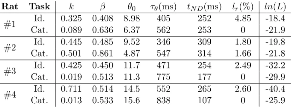
3.1 DDM best-fit parameters for individual rats and tasks. . . . 51 3.2 DDM best-fit parameters for identification and
categoriza-tion tasks. . . 53 3.3 DDM goodness-of-fit for identification and categorization
tasks. . . 55 3.4 Parameters for DDM convolved with Gaussian kernel. . . . 59 3.5 Parameters for DDM with random weights noise. . . 61 4.1 Spearman’s rank correlation statistics for session-by-session
performance and individual rats. . . 68 4.2 Individual rats’ Spearman’s rank correlation statistics for
choice bias on a day-by-day basis. . . 69 5.1 Fitted parameters and comparative goodness-of-fit for all
versions of DDM used in this thesis. . . 95 6.1 Spearman’s rank correlation between GLM estimators for
OFC data. . . 125 6.2 Spearman’s rank correlation between GLM estimators for
List of Figures
2.1 Two-alternative odor choice task. . . 29
2.2 Stimulus design and task differences. . . 31
2.3 Tasks training and testing time-line. . . 33
2.4 Comparison between odor identification and mixture cate-gorization tasks. . . 37
2.5 Odor mixture identification task. . . 39
3.1 Drift-diffusion model. . . 43
3.2 Three-layered DDM model. . . 45
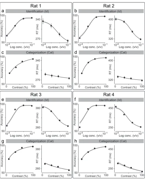
3.3 Individual behavioral data and DDM fits. . . 52
3.4 Overall behavioral data and DDM fits. . . 54
3.5 Failure to fit performance in one task and predict the other. 56 3.6 Failure to simultaneously fit performance on identification and categorization tasks with DDM. . . 57
3.7 DDM convolution with Gaussian kernel. . . 60
3.8 DDM with random trial-by-trial weight fluctuations. . . 62
3.9 DDM with random trial-by-trial weight fluctuations fits both tasks. . . 63
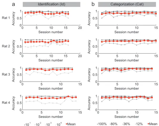
4.1 Session-by-session stable performance in behavioral data. . 70
4.2 Individual rats’ session-by-session bias. . . 71
4.4 Reward history effects are still present despite overall
sta-bilized performance. . . 75
4.5 Updating curves for change in choice bias after an error response for both tasks. . . 76
4.6 Conditional psychometric curves for trialsT andT−2 after an easy trial error in identification task. . . 77
4.7 Updating curves for change in choice bias after rewarded trials for all individual rats and tasks. . . 78
5.1 DDM with reward bias. . . 84
5.2 DDM+bias fails to predict categorization task. . . 87
5.3 DDM with bias and stimulus learning. . . 89
5.4 Stimulus learning influence on identification task. . . 92
5.5 Fitting landscapes for learning parameter. . . 94
5.6 Fitting landscapes for RL-DDM . . . 95
5.7 DDM with bias and stimulus learning explains identifica-tion and categorizaidentifica-tion task simultaneously. . . 97
5.8 DDM+bias and RL-DDM predictions for full updating curves. 98 5.9 DDM+bias with random weights fluctuations predictions for changes in choice bias. . . 99
5.10 RL-DDM predictions for changes in reaction times. . . 100
5.11 Weight fluctuations amplify errors in categorization task. . 104
5.12 Model weights correlate with rats’ local bias. . . 105
5.13 Two-race model with learning also explains identification and categorization task simultaneously. . . 108
6.1 RL-DDM predictions for change in evidence rate after trial outcome. . . 113
6.2 Time wagering confidence task. . . 117
6.4 Average firing rate GLM parameters for current choice and previous trial outcome. . . 121 6.5 PETHs for example OFC cell modulated by previous outcome.123 6.6 PETHs for example VS cell modulated by previous outcome.124 6.7 Average firing rate GLM parameters for current choice and
previous trial outcome interacting with stimulus difficulty. . 126 6.8 Slope of linear regressions for GLM difficulty parameters. . 127 6.9 PETHs for example OFC cell modulated by previous
out-come and difficulty. . . 128 6.10 PETHs for example VS cell modulated by previous outcome
Abbreviations
2RM . . . Two-Race accumulation Model
BIC . . . Bayesian Information Criterion
DDM . . . Drift-Diffusion Model
DDM+bias . . . Drift-Diffusion Model with choice Bias
DM . . . Decision-Making
DV . . . Decision Variable
EDM . . . Economical Decision-Making
EOG . . . Electro-OlfactoGram
FOF . . . Frontal Orienting Fields
GLM . . . Generalized Linear Model
LIP . . . Lateral Intra-Parietal area
MC . . . Mitral Cell
ML . . . Matching Law
NS . . . Nervous System
OB . . . Olfactory Bulb
OFC . . . Orbito Frontal Cortex
OT . . . Olfactory Tubecule
PIR . . . PIRiform cortex
PPC . . . Posterior Parietal Cortex
QM . . . Quantum Mechanics
RDK . . . Random-Dot Kinematogram
RL . . . Reinforcement Learning
RL-DDM . . . Reinforcement Learning Drift-Diffusion Model
RT . . . Reaction Time
SA . . . Sequential Analysis
SAT . . . Speed-Accuracy Tradeoff
SDT . . . Signal Detection Theory
VS . . . Ventral Striatum
Chapter 1
Introduction
“Every puzzle has an answer”
1.1
Chapter Summary
In this introduction we will address the topics of perceptual and economi-cal decision-making. The goal of this introduction is to give the reader an overview and intuition of what are the challenges present while the brain tries to categorize perceptual stimuli.
To do so we divided this Chapter in 4 sections:
• Randomness, noise and the brain – in which we approach the
subject of noise, uncertainty and random events and how the brain might cope with different sources of noise.
• Sensory uncertainty – a general review on the subject of sensory noise and its role in perceptual decision-making.
• Actions, categories and the ever-changing environment– an
introduction on the subject of economical decision-making, with a particular focus on potentially extra sources of “noise”.
• Conceptual introduction and organization of the thesis –
1.2
Introduction
T
he room is dark. You have no idea of what is this place, only darkness surrounds you. Slowly, an outline is drawn in the hori-zon and a beam of light propagates through the floor. You realize that there is a door, a door that is slightly ajar. You open it. You are almost blinded by the light.As you cross the edge of the door you look around you. In front of you, a glade propagates into a forest full of strange colored and weird shaped trees, plants and animals. You have never experienced anything like this. Millions of photons bombard your retina; thousands of chemicals stimulate your olfactory receptors. As you walk through this forest you touch everything, anything that comes to reach. The textures of a leaf that grasped your attention feel funny, pointy while they look smooth. The patterns create a sensation that you’re not familiar with. Your neurons are firing in ways that you have never felt before.
You see a strange fruit sitting in a brunch two feet away. You walk, but suddenly your legs are heavy, you take longer than you realize to reach this fruit. You feel massive, as if any small movement requires the strength of the world. You were so distracted as you left the room that you did not realize that even gravity has changed. Two feet, how hard can it be?
your hand perfectly. This is strange, you think to yourself. But you are so terribly thirsty, and so so hungry. You eat the strange fruit.
The effects are almost immediate, you feel massively rewarded; you have never felt anything like this. If words could describe your feelings, you would say that this fruit felt like fresh silk going down your throat. You want more and more of this fruit.
Or maybe the effects are just the opposite. You feel terribly sick after some minutes. You see everything move, rotations occur around you and you’re the center axis. A massive bush that was sitting right next to you (“was it always there!?”) starts to morph into a face; a green and blue and black monster looks straight at you with his bloody eyes. You panic, what is this? What is happening to me? You try to run but you can’t. The face dissolves and transforms itself into thousands of snakes that twist and twirl in your direction. As the first touches your skin you see that it was naught but a branch blown by wind.
You are now asked to remove your virtual-reality goggles. You now remember that this was all part of a simulation. But you will be asked to do it again.
Did you memorize the exact hue of that green-blue color? Will you pick it up again?
This small piece of fiction is meant to illustrate the potential within our brains to extract meaning and categories from sensory input. But it also metaphorically depicts the fundamental question of perceptual decisions-making and that lives at the heart of this thesis: what modulates our percepts?
1.3
Randomness, noise and the brain
Randomness is defined as the lack of pattern or, more importantly for the case of neuroscience, lack of predictability in events. Events that are un-intelligible in pattern (both spatially or temporally) are considered to be random. Randomness is considered to be a measurement of uncertainty in a particular outcome and has been applied to concepts of chance, prob-ability and information theory (Bennett, 2009).
In the field of physics, the idea of random motion was fundamental for the development of statistical physics (Landau & Lifshitz, 2013). The incorporation of such concepts was paramount for the explanation of phe-nomena observed in thermodynamics and chemistry. Randomness is also key for the field of quantum mechanics (QM). Take the example of an unstable atom in a controlled environment. According to QM, its decay cannot be predicted efficiently, only the probability of it decaying in a given amount of time. QM works at the level of event probabilities and not at the resolution of individual outcomes (Feynman, Leighton, & Sands, 1963).
Rosen, 1935). These theories posit that apparent random processes con-tain variables from statistical distributions that are working behind the scenes, and thus not immediately accessible or visible.
In biology, randomness has been described to exist in evolution. In par-ticular genetic mutations have been thought to be random and an injector of variability upon which natural selection works on (Hastings, Lupski, Rosenberg, & Ira, 2009; Abby & Daubin, 2007). The environment would then work as the driving force behind deterministic characteristics arising (Klasson & Andersson, 2004). But is that always the case? Alternative mechanisms for non-random induced genetic variability in a population have been presented in the past (Wright, 2000; Martincorena, Seshasayee, & Luscombe, 2012).
In neuroscience, noise has been used to define unpredictable events that exist in the environment (Waiblinger, Brugger, Whitmire, Stanley, & Schwarz, 2015; Buzs´aki, Peyrache, & Kubie, 2015), in human and an-imal behavior (Schmidt, Zelaznik, Hawkins, Frank, & Quinn, 1979; de C. Hamilton, Jones, & Wolpert, 2004; Lum, Zhurov, Cropper, Weiss, & Brezina, 2005; Hooper, Guschlbauer, von Uckermann, & Buschges, 2006) and in neural activity (Deneve, Latham, & Pouget, 2001; Fitzpatrick, Batra, Stanford, & Kuwada, 1997; Kasamatsu, Polat, Pettet, & Norcia, 2001; Rolls & Deco, 2010; Shadlen, Britten, Newsome, & Movshon, 1996; Stocker & Simoncelli, 2006). Despite this, opposing ideas and theories have been brought forward that support (Faisal, Selen, & Wolpert, 2008) or challenge (Beck, Ma, Pitkow, Latham, & Pouget, 2012) the true nature of these sources of noise.
Bengson, Kelley, Zhang, Wang, & Mangun, 2014). In this work, we aim to help shed light on some of these issues. We aim to understand the unpredictable/random/variable events in rodents performing a perceptual decision-making (PDM) task. In particular, we are interested in identify-ing what types of uncertainty does the nervous system (NS) have to cope with, and why or in which occasions they might be limiting behavior and respective performance.
1.3.1 Optimality
works (Von Neumann, 1956; Laughlin & Sejnowski, 2003). However, a different interpretation for the same result is that monkeys are in fact in-ferring sub-optimally (Beck et al., 2012). In that particular study, Beck et al. suggest that all noise might be purely driven by sensors and amplified by choices that suffered deterministic (but suboptimal) approximations.
It is clear that individuals are not optimal in some particular cases (Yu & Cohen, 2008). The instructions given or the environmental set up might make the same subject oscillate from an observable optimal strat-egy to a non-optimal one (Summerfield & Tsetsos, 2012). In particular, a study in humans showed that subjects exposed to a rapidly changing perceptual environment were best explained by a non-optimal strategy (working memory rather than Bayesian inference; Summerfield, Behrens, & Koechlin, 2011). Considering that many results have showed that hu-mans and monkeys can classify optimally visual information (Stocker & Simoncelli, 2006; Michel & Jacobs, 2008; Anderson, 1991; Ashby & Gott, 1988), one is led to conclude that the nature of the task at hand plays a significant role in understanding the strategies conducted by the NS. The gaps between optimal and non-optimal strategies might tell us more of how the brain copes with the external environment and help explain part of the observed variability of many tasks (Summerfield & Tsetsos, 2012). Last but not least, if one considers the artificial setting of a controlled lab environment and its intrinsic difference with bona fide habitats, then one is led to the conclusion that these studies might help shed light on what are the significant evolutionary traits that emerged in the NS.
1.4
Sensory uncertainty
to classify noisy sensory information. Here we explore how that sensory uncertainty has been defined and addressed in the field.
1.4.1 Perceptual decision-making
PDM is the process by which sensory information is used to guide be-havior toward the external world. This involves gathering, evaluating and integrating information that was acquired through the senses. This information is then taken into account to produce judgments about the environment and conduct motor responses (Gold & Shadlen, 2007).
1.4.2 Signal detection theory
The study of perception and psychophysics has been a focus of decision theory since the XIX century (Fechner, 1948; Smith, 1994). Mathematical descriptions have been brought forward ever since, being signal detection theory (SDT) one of most historically relevant (Green & Swets, 1966).
SDT describes the process wherein inherent sensitivity of subjects to relevant stimuli is combined to generate choices, setting a framework to understand performance in perceptual tasks (Green & Swets, 1966). Ac-cording to SDT, the decision-maker obtains an observation of noisy evi-dence from the stimulus, which gives rise to the DV that is then evaluated according to the decision rule. In simple binary decisions, the DV is typi-cally related to the likelihood ratio of the different alternatives, and then compared to a given criterion. This criterion can also incorporate differ-ent priors (through Bayes rule, for instance) and value, allowing a flexible structure to hypothesize about PDM (Gold & Shadlen, 2007; Glimcher & Fehr, 2014).
1.4.3 Sequential analysis
framework is that it allows predictions of how response times are generated (Edwards, 1965).
Several versions of sequential sampling models have been instantiated in the past (Gold & Shadlen, 2007; Luce, 1986; Townsend & Ashby, 1983; Vickers, 1970; Vickers, Carterette, & Friedman, 2014; Usher & McClel-land, 2001; Ratcliff & Smith, 2004). A particular important instantiation are random walk models. In these models the DV is a cumulative sum of evidence over discrete time steps. If the evidence is the logarithm of the likelihood ratio, then this process corresponds to the statistically-optimal Sequential Probability Ratio Test (Wald & Wolfowitz, 1949). Instead, if the evidence is sampled from a Gaussian distribution in infinitesimal time steps, the process is termed diffusion with drift or bounded diffusion (Ratcliff, 1978).
While many models provide an account of either RT (Townsend & Ashby, 1983) or accuracy (Green & Swets, 1966), sequential sampling models relate shapes of RT distributions with probabilities of correct and incorrect responses, thereby explaining how RT and choice accuracy jointly vary as a function of the experimental conditions of interest. An impor-tant part of SA is that it allows quantification of the noise associated to psychophysical processes. Additionally, SA can be used to model and ex-plain neurophysiological data (Gold & Shadlen, 2007; Sajda, Philiastides, Heekeren, & Ratcliff, 2011). For instance, recordings of neural activity in primates performing a random dot kinematogram (RDK) task have shown neural correlates resembling SA DVs (Roitman & Shadlen, 2002).
1.4.4 Accumulator models and Speed-accuracy tradeoffs
Dornhaus, 2003; Histed, Carvalho, & Maunsell, 2012; Bowman, Kording, & Gottfried, 2012; Brunton, Botvinick, & Brody, 2013; Gold & Shadlen, 2007; Ratcliff & McKoon, 2008). Simple theoretical models of evidence accumulation based on a random walk-to-bound have been successful in critical aspects of the performance of psychophysical tasks, capturing the dependence of accuracy (psychometric) and reaction time (chronometric) functions. Key elements of these models have begun to be tested both by searching for neural activity corresponding to model variables (Kiani, Hanks, & Shadlen, 2008; Roitman & Shadlen, 2002; Hanks, Ditterich, & Shadlen, 2006; Erlich, Brunton, Duan, Hanks, & Brody, 2015; Hanks et al., 2015) and by the use of more sophisticated task design and modeling (Brunton et al., 2013; Zariwala, Kepecs, Uchida, Hirokawa, & Mainen, 2013). Yet substantial ambiguity remains concerning nearly all critical features of this class of models, including the basic mechanisms support-ing integration, how a bound is determined and the origins of apparent randomness.
expla-nation for differences seen across similar studies, although manipulation of motivation in one case failed to support this explanation (Zariwala et al., 2013). An alternative proposal is that differences in reaction time (RT) arise from different computational requirements of different tasks (Uchida, Kepecs, & Mainen, 2006; Zariwala et al., 2013; Summerfield & Tsetsos, 2012). Given that species, modality and task structure all vary across the different studies in question, distinguishing amongst these possibili-ties from existing data is difficult.
1.5
Actions, categories and the ever-changing
environment
Although sensory information is ambiguous in PDM, a problem that arises from a simplistic approach is that a significant subset of these tasks present over-trained subjects that have developed a clear idea of how the sensory-to-action contingencies should work (Britten, Shadlen, Newsome, & Movshon, 1993). It is the identity of the stimulus, and thus, sensory uncertainty that is driving decisions in these type of tasks. However, what happens when these contingencies are not clear? How does a subject pick from a set of actions when perceptual categories and respective context might be changing on a trial-by-trial basis? Or when a subject believes
the environment to be changing?
Here we explore how other sources of uncertainty (that also exist in PDM, see Busse et al., 2011 for an example) have been defined and ad-dressed in the field of economic decision-making (EDM).
1.5.1 Matching law
(Nomoto & Lima, 2015), or social interactions (Marquez, Rennie, Costa, & Moita, 2015), have all been used as rewards for an animal. On the opposite scale, punishments have also been used as they generate negative action values that shun particular decisions (Paton, Belova, Morrison, & Salzman, 2006). A logical starting point is to consider that the net value of a particular decision is dictated by the needs that an agent wishes to satisfy. By this premise, an animal will choose to perform certain actions in detriment of others, so to maximize the rate of obtained reward - this is known as the matching law (ML).
The ML was first formulated by Herrnstein (1961) following an ex-periment with pigeons on concurrent variable interval schedules. Pigeons were presented with two buttons in a box, each with varying rates of food reward. The pigeons tended to peck the button that yielded the greater food reward more often than the low reward option. The ratio of their rates to the two buttons matched the ratio of reward rates on the two buttons. In operant conditioning, ML is then defined as the quantitative relationship between the relative rates of response and reinforcers in a concurrent reinforcement schedule. In the case of the pigeons, if the two response alternatives A and B are offered, the ratio of response rates to
A and B equals the ratio of reinforcements yielded by each response:
RA
RB
= rA
rB
(1.1) being R the amount of responses for a particular side and r the reward frequency of that same option.
1.5.2 Reinforcement learning
However, ML does not address the issue of how these action values are accessed by the agent or even implemented in the brain.
When it comes to classical conditioning, reinforcement learning (RL) models have been very successful in describing EDM. RL emerged from the fields of experimental psychology (Rescorla & Wagner, 1972) and machine learning (Sutton & Barto, 1998), and it describes a mechanism for how the value of a particular stimulus or action is learned. Its basic premise is that values are updated by considering a prediction error (i.e., how surprising a given outcome is) and the weight that that particular error should have (learning rate). A simple version of these class of models is to consider the trial-by-trial learning rule known as the Rescorla-Wagner delta rule:
w7→w+αδµ (1.2) whereαis the learning rate, which can be interpreted as the associability of the stimulus, µ, with the reward; andw the weight that maps a stimulus to an action. The crucial term here is to consider the prediction error,
δ =r−wµ, which dictates how far of predicting the reward,r, might the stimulus be (or not) and thus updated accordingly.
1.5.3 Value-based decision-making
2007). In these particular cases the identity of the stimulus was clear to the agent, but its relative value and prospective action were uncertain (Louie, Khaw, & Glimcher, 2013).
In most EDM tasks the choice process is usually modeled by assum-ing a greedy policy (the most valuable option available to the agent) or by a “softmax” function that permits some level of noise in the deci-sion process. However, these models exist at a meta-process modeling level and lack process implementation and development (Lindland, Sin-dre, & Solvberg, 1994). Namely, they lack mechanisms that explain how a particular stimulus might be integrated, compared and classified by a neural network, and thus dictate the action to pursue. Fusing RL models with accumulator models might help shed light on some of these issues (Summerfield & Tsetsos, 2012).
1.5.4 Orbitofrontal cortex and ventral striatum
One important issue in both PDM and EDM is the neural implementa-tion of these conceptual models, specially when considering the crosstalk between the two fields, as we propose to do here.
These findings are in concordance with the view of OFC as playing a central role in goal monitoring (Padoa-Schioppa & Assad, 2008; Schoen-baum, Takahashi, Liu, & McDannald, 2011; Takahashi et al., 2013). OFC activity was also found to be encoding decision confidence in rats per-forming an odor mixture categorization task (Kepecs, Uchida, Zariwala, & Mainen, 2008).
Evaluation, or performance monitoring, is necessary to analyze the efficacy or optimality of a decision with respect to its goals (Shadlen & Kiani, 2013). OFC is particularly important for reward-based behaviors when values are inferred, for instance using model-based RL algorithms (Daw & Doya, 2006). Additionally, OFC has been shown to keep track of absolute stimulus value (Kable & Glimcher, 2009) and to encode value in a “common currency” that allows comparison between variables that exist at different domains (Summerfield & Tsetsos, 2012).
1.6
Conceptual introduction and organization of
the thesis
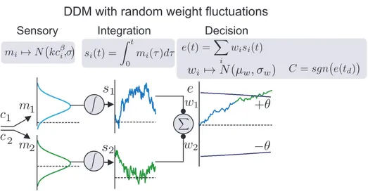
In theoretical models of evidence accumulation, the chief source of uncer-tainty is stochasticity in incoming sensory evidence, modeled as Gaussian white noise around the true mean evidence rate (Ratcliff, 1978; Ratcliff & Smith, 2004). It is this rapidly fluctuating noise that accounts for the ben-efits of temporal integration. The nature and implications of other sources of variability have also been considered in diffusion models (Ratcliff, 1978; Ratcliff & Smith, 2004; Ratcliff & McKoon, 2008; Mulder, Wagenmakers, Ratcliff, Boekel, & Forstmann, 2012; Brunton et al., 2013; Fr¨und, Wich-mann, & Macke, 2014), including variability in starting position (Mulder et al., 2012), variability in non-accumulation time (Ratcliff & Smith, 2004) and variability in threshold or “bound” (Ratcliff, 1978).
A potentially important source of uncertainty is trial-by-trial fluctua-tions in the mean rate of evidence accumulation. Such fluctuafluctua-tions would correspond to variability in the mapping of sensory data onto evidence for a particular choice direction (Gold, Law, Connolly, & Bennur, 2008; Beck et al., 2008). It has been hypothesized that such fluctuations would introduce errors that, unlike rapid fluctuations, could not be mitigated by temporal integration and would therefore curtail the benefits of ev-idence accumulation (Uchida et al., 2006; Zariwala et al., 2013). Such “boundary” (not to be confused with the stopping “bound” in accumula-tion models) variability might differentially affect different sort of decision tasks, being particularly important when the mapping from stimulus to action must be learned de novo, such as in a categorization task (Uchida et al., 2006; Zariwala et al., 2013).
mix-ture categorization task (Uchida & Mainen, 2003) in which the difficulty was increased by making the stimuli closer to a decision category bound-ary. The second was an odor identification task in which the difficulty was increased by lowering stimulus concentration. We found that the change in reaction times over a given range of accuracy differed markedly between the two tasks, despite being tested in the same subjects with all other task variables constant. We sought to obtain direct evidence that such bound-ary fluctuations limits perceptual decision performance and contributes to task differences in SAT. To do so, we considered the hypothesis that these boundary fluctuations reflect a form of on-going RL (Rescorla & Wagner, 1972; Sutton & Barto, 1998). Although perceptual choices are normally considered to be driven by sensory information, according to RL, choices should be driven by expected rewards. RL is a normative theory that posits that agents learn the expected values of different choice options from the history of their outcomes and that options are chosen so as to maximize those values (Rescorla & Wagner, 1972; Sutton & Barto, 1998). It is known that reward history can produce biases that effect perceptual decisions, contributing to a reduction in decision accuracy (Busse et al., 2011). If an RL mechanism is responsible, then these reward-dependent choice biases ought to exhibit specific patterns that would depend on the magnitude of the reward prediction errors generated by different stimu-lus/choice/outcome combinations.
task. Critically, the introduction of RL predicted a history-dependence of trial-by-trial choice biases whose specific pattern and magnitude were closely, qualitatively and quantitatively, matched to the data.
Lastly, by considering the involvement of both OFC (Kepecs, Uchida, Zariwala, & Mainen, 2008; Lak et al., 2014) and VS (Costa, 2015) in odor categorization, we devised a generalized liner model and applied it to previously acquired data (Costa, 2015) in search of correlates associated to changes predicted by our RL model. We found that both OFC and VS neuronal activity is modulated by the outcomes of previous trials. In particular, OFC showed modulated responses dependent on the categorical uncertainty of to the stimulus at hand.
These findings support the notion that RL amplifies sensory variability, producing an additional source of decision variability without implying stochastic internal processes (Beck et al., 2012).
To better present our findings we divided this thesis in 6 additional Chapters.
• Chapter 2 – where the behavioral results that comprise this the-sis are presented and the difference between odor identification and mixture categorization explained.
• Chapter 3– in which the issue of sensory uncertainty is addressed via the implementation of accumulator models, and why there is a need for an extra source of “noise”.
• Chapter 4– in which we analyzed the effects of rewards and errors in on-going performance and local changes of choice-bias.
from and how it might be amplified by an RL rule, we are able to not only fit the behavioral data but also predict an additional dataset.
• Chapter 6 – in this chapter we tested for the presence of neural signatures of weight updating that were expected by our RL model. We saw both OFC and VS presented significant effects, although different in nature regarding stimulus uncertainty.
Chapter 2
Odor identification and
mixture categorization
“We are our choices”
2.1
Chapter Summary
In this Chapter we present the behavioral data that serve as the backbone of this thesis. The Chapter is divided in three sections:
• Introduction – a brief introduction on the subject of
Speed-accuracy tradeoffs.
• Animal subjects – where behavioral methodology details such as
differences in tasks, training and testing are explained.
2.2
Introduction
T
he quote “Fast is fine, but accuracy is everything” has been at-tributed to famous gambler and deputy sheriff Wyatt Earp in var-ious contexts. Notorvar-iously, it was replicated by American actor Kevin Costner in the movie of the same name (Kasdan, 1994). However, many historians believe that the sentence originated from a Greek student of Socrates, Xenophon. Regardless of the dispute, the fact that one lived in the XIX century while the other in 300 BC tells us that the interplay between accuracy and speed has been a philosophical point of discussion throughout the years.Relationships between accuracy and speed of decision-making, or speed-accuracy tradeoffs (SATs), have been extensively studied in hu-mans and other species including monkeys, rodents and insects (Gold & Shadlen, 2007; Luce, 1986; Palmer et al., 2005; Roitman & Shadlen, 2002; Uchida, Poo, & Haddad, 2014; Chittka et al., 2003; Chittka, Skorupski, & Raine, 2015; Uchida & Mainen, 2003; Abraham et al., 2004; Rinberg et al., 2006b; Histed et al., 2012; Zariwala et al., 2013; Bowman et al., 2012). In many ways Earp’s quote seems to be true. Still, many other situations might favor fast decisions such as environments in which resources are scarce (competition) or contexts of predator presence (survival; Dawkins, 2004). It would only be natural to assume that many evolutionary pres-sures potentiated fine tuning of SATs (Gold & Shadlen, 2007; Dawkins, 2004).
an odor mixture discrimination task (Uchida & Mainen, 2003). It is not known what accounts for such different degrees of SAT observed across different studies.
Motivation for speed vs. accuracy is thought to be a key parameter affecting SAT (Khan & Sobel, 2004) and is a possible explanation for the differences observed across similar studies showing SAT of smaller (Uchida & Mainen, 2003) or larger (Abraham et al., 2004; Rinberg et al., 2006b) magnitudes. Two alternative possibilities are that longer SATs reflect neu-ral mechanisms that are species-specific and/or sensory modality-specific. An additional explanation is that SAT differences arise from differences in the underlying computational requirements of different decision-making tasks (Zariwala et al., 2013). Given that species, modality, task structure all vary across the different studies in question, these possibilities are not distinguishable from existing data.
Our strategy was to compare SATs in two behavioral tasks that were identical except for the nature of the stimuli that gives rise to task dif-ficulty. The first was a stimulus noise driven task in which the difficulty was increased by lowering stimulus concentration. We named this task “odor identification”. The second was an odor mixture categorization task (Uchida & Mainen, 2003) in which the difficulty was increased by making the stimuli closer to a decision or category boundary. Thus, by having the same subjects performing two tasks that were different only for the set of stimuli, and by holding species, modality and motivation, we were in a condition that allowed us to test if SAT was dependent on the nature of the task. Our motivation was to create two extremely sim-ilar tasks that required different strategies and in that way explore and understand what dictates SAT.
that exist between the two tasks and that motivated the central topic of this study.
2.3
Animal subjects
Four Long Evans rats (200-250 g at the start of training) were trained and tested in accordance with European Union Directive 86/609/EEC and approved by Direc¸c˜ao-Geral de Veterin´aria (DGV) of Portugal. Rats were trained and tested on three different tasks: (1) a two-alternative choice odor identification task; (2) a two-alternative choice odor mixture categorization task (Uchida & Mainen, 2003); and (3) a two-alternative choice “odor mixture identification” task. The same rats performed all three tasks that differ on the nature of the presented stimulus while all other task variables were held constant (Figure 2.1). Rats were pair-housed and maintained on a normal 12 hr light/dark cycle and tested during the daylight period. Rats were allowed free access to food but were water-restricted. Water was available during the behavioral session and for 20 minutes after the session at a random time as well as on non-training days. Water availability was adjusted to ensure animals maintained no less than 85% of ad libitum weight at any time.
2.3.1 Training and testing apparatus
a
Odor Port Choice Port
Choice Port Trial start
Trial start
Stimulus Choice Outcome
Correct
Error
OH
Odor Port
Odor Valve
Choice Port
Water Valve d
odor RT MT
d
water dinter-trial
b
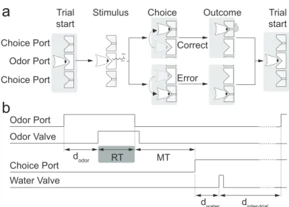
Figure 2.1. Two-alternative odor choice task. (a)Rats were trained in a behavioral box to signal a choice between left and right port after sampling a central odor port. The sequence of events is illustrated using a schematic of the ports and the position of the snout of the rats. (b) Illustration of the timing of events in a typical trial. Nose port photodiode and valve command signals are shown (thick lines). A trial is initialized after a rat pokes into a central odor port. After a randomized delaydodora pure odor
or a mixture of odors is presented, dependent of the task at hand. The rat can sample freely and respond by moving into a choice port in order to get a water reward. Each of these ports is associated to one of two odors – odor A ((R)-()-2-Octanol) and odor B ((S)-(+)-2-Octanol). Highlighted by the grey box, reaction time (RT) is the amount of time the rats spend in the central odor port.
M. Recchia. During training and testing the rats alternated between two different boxes.
The test odors were S-(+) and R-(-) stereoisomers of 2-octanol, cho-sen for their identical vapor pressures and similar intensities (Uchida & Mainen, 2003; Taniguchi, Kashiwayanagi, & Kurihara, 1992; Pierce, Zeng, Aronov, Preti, & Wysocki, 1995; Laska, Psychologie, M¨unchen, & M¨unchen, 2004). In the odor identification task, difficulty was manipu-lated by using different concentrations of pure odors, ranging from 10−4
to 10−1 (v/v) (Figure 2.2a). The different concentrations were produced by serial liquid dilution using an odorless carrier, propylene glycol (1,2-propanediol). In the odor mixture categorization task, we used binary mixtures of these two odorants at different ratios, with the sum held con-stant: 0/100, 20/80, 32/68, 44/56 and their complements (100/0, etc.; Figure 2.2b). Difficulty was determined by the distance of the mixtures to the category boundary (50/50), denoted as “mixture contrast” (e.g. 80/20 and 20/80 stimuli correspond to 60% mixture contrast). Choices were rewarded at the left choice port for odorant A (identification task; Figure 2.2c,d) or for mixtures A/B >50/50 (categorization task; Figure 2.2e,f) and at the right choice port for odorant B (identification task) or for mixtures A/B <50/50 (categorization task). In both tasks, the set of eight stimuli were randomly interleaved within the session. During testing, the probability of each stimulus being selected was the same.
Identification (Id.) Task
Categorization (Cat.) Task
c
d
a
b
e
10-4 Odor A 10-1
Log conc. (v/v)
10-1 10-4 L o g co n c. (v/ v) O d o r B
f
10-4 Odor A 10-1
Log conc. (v/v)
10-1 10-4 L o g co n c. (v/ v) O d o r B B A 0 100 32 68 44 56 56 44 68 32 100 0 20 80 80 20 B A 0 10 0 0
0 0 0
0
0 -¹10-²10-³10-⁴
10-⁴ 10-³10-²10-¹
0.1 0 0.1 Odor A conc. (v/v) O d o r B co n c. (v/ v) 0.1 0 0.1 Odor A conc. (v/v) O d o r B co n c. (v/ v)
Figure 2.2. Stimulus design and task differences. (a,b) In the odor de-tection task, the odorants were presented independently at concentrations ranging 10−1 to 10−4 (v/v) and sides rewarded accordingly (a). For the mixture categorization task, the two odorants were mixed in different ra-tios presented at a fixed total concentration of 10−1, and rats were
For all the different experiments, four of the eight stimuli presented in each session were rewarded on the left (A > B) and the other four were rewarded on the right (A < B). Each stimulus was presented with equal probability and corresponded to a different filter in the manifold.
The training sequence consisted of: (I) handling (2 sessions); (II) water port training (1 session); (III) odor port training, in which a nose poke at the odor sampling port was required before water was available at the choice port. The required center poke duration was increased from 0 to 300 ms (4 - 8 sessions); (IV) introduction of test odors at a concentration of 10−1, rewarded at left and right choice ports according to the identity of the odor presented (1 - 5 sessions); (V) introduction of increasingly lower concentrations (5 - 10 sessions); (VI) training on odor identification task (10 - 20 sessions); (VII) testing on odor identification task (14 - 16 sessions); (VIII) training on mixture categorization task (10 - 20 sessions); (IX) testing on mixture categorization task (14 - 15 sessions); (X) testing on mixture identification task (12 - 27 sessions) (Figure 2.3).
During training, in phases VI and VIII, we used adaptive algorithms to adjust the difficulty and to minimize bias of the animals. We computed an online estimate of bias:
bt= (1−τ)Ct+τ bt−1 (2.1)
where bt is the estimated bias in the current trial, bt−1 is the estimated
bias in the previous trial, Ct is the choice of the current trial (0 if right,
1 if left) and τ is the decay rate (τ = 0.95 in our experiments). The probability, p, of being presented with a right-side rewarded odor was adjusted to counteract the measured bias using:
pR= 1−
1
II
1
I
2
III
4 - 8 sessions
IV
1 - 5
V
5 - 10 sessions
VI - Id training
10 - 20 sessions
VII - Id testing
14 - 16 sessions
VIII - Cat training
10 - 20 sessions
IX - Cat testing
14 - 15 sessions
X - Mixture Id testing
12 - 27 sessions
Figure 2.3. Tasks training and testing time-line. (I) Handling (2 sessions). (II) Water port training (1 session). (III) Odor port training (4 - 8 ses-sions). (IV) Pure odor training (1 - 5 sesses-sions). (V) Introduction of lower concentrations (5 10 sessions). (VI) Odor identification training (10 -20 sessions). (VII) Odor identification testing (14 - 16 sessions). (VIII) Mixture categorization training (10 - 20 sessions); (IX) Mixture categorization testing (14 15 sessions). (X) Mixture identification testing (12 -27 sessions). Each session represents a different day. Grey boxes highlight the behaviorial data presented in Chapter 2 to 5.
where b0 is the target bias (set to 0.5), and γ (set to 0.25) describes the
degree of non-linearity.
Analogously, the probability of a given stimulus difficulty was depen-dent on the performance of the animal, i.e., the relative probability of difficult stimuli was set to increase with performance. Performance was calculated in an analogous way as Equation 2.1 at the current trial but ct
became rt – the outcome of the current trial (0 if error, 1 if correct). A
difficulty parameter,δ, was adjusted as a function of the performance,
δt+1=−1 +
2
where p0 is the target performance (set to 0.95). The probability of each
stimulus difficulty,ϕ, was drawn from a geometric cumulative distribution function (GEOCDF, Matlab):
ϕt+1 =
1−GEOCDF i,|δt+1|
PN
j=11−GEOCDF j,|δt+1|
(2.4)
where N is the number of stimulus difficulties in the session, and takes a value from 2 to 4 (when N = 1, i.e. only one stimulus difficulty, this algorithm is not needed); i corresponds to the stimulus difficulty and is an integer from 1 to 4 (when δ >0, the value 1 corresponds to the easiest stimuli and 4 to the most difficult one, and vice-versa whenδ <0). In this way, when|δ|is close to 0, corresponding to an average performance close to 0.95, the distribution of stimuli was close to uniform (i.e. all difficulties are equally likely to be presented). When performance is greater, then the relative probability of difficult trials increased; conversely, when the performance is lower, the relative probability of difficult trials decreased. Training phases VI and VIII were interrupted for both tasks when number of stimulus difficulties N = 4 and difficulty parameter δ stabilized on a session-by-session basis.
Each rat performed one session of 90 – 120 minutes per day (250 -400 trials), 5 days per week for a period of ∼120 weeks. During test-ing, the adapting algorithms were turned off and each task was tested independently.
2.3.2 Reaction time paradigm
The timing of task events are illustrated in Figure 2.1. Rats initiated a trial by entering the central odor-sampling port, which triggered the delivery of an odor with delay (dodor) drawn from a uniform distribution
onset. Rats could exit from the odor port at any time after odor valve opening, and make a movement to either of the two reward ports. Trials in which the rat left the odor sampling port before odor valve opening (∼4% of trials) or before a minimum odor sampling time of 100 ms had elapsed (∼1% of trials) were considered invalid. Odor delivery was terminated as soon as the rat exited the odor port. Reaction time (the odor sampling duration) was calculated as the difference between odor valve actuation until odor port exit (Figure 2.1b) minus the delay from valve opening to odor reaching the nose. This delay was measured with a photo ionization detector (mini-PID, Aurora Scientific, Inc) and had a value of 53 ms.
Reward was available for correct choices for up to 4 s after the rat left the odor sampling port. For correct trials, water was delivered from gravity-fed reservoirs regulated by solenoid valves after the rat entered the choice port, with a delay (dwater) drawn from a uniform distribution
with a range of [0.1, 0.3] s. Trials in which the rat failed to respond to one of the two choice ports within the reward availability period (0.5% of trials) were also considered invalid. Reward amount (wrew), determined
by valve opening duration, was set to 0.024 ml and calibrated regularly. A new trial was initiated when the rat entered odor port, as long as a minimum interval (dinter−trial), of 4 s from water delivery, had elapsed.
Error choices resulted in water omission and a “time-out” penalty of 4 s added to dinter−trial. Behavioral accuracy was defined as the number
of correct choices over the total number of correct and incorrect choices. Invalid trials (in total 5.8±0.8% of trials, mean±SEM, n = 4 rats) were not included in the calculation of performance accuracy or reaction times.
2.3.3 Statistical and behavioral analysis
2.4
Behavioral results
2.4.1 Odor identification versus odor categorization
We trained Long Evans rats on two different two-alternative choice olfac-tory reaction time tasks that were similar except for the stimulus concen-trations (Figure 2.1).
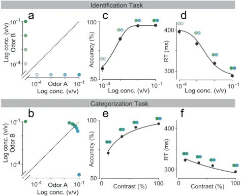
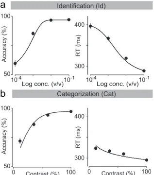
In the first task, “odor identification”, a single odor was presented at any given trial and we manipulated difficulty by diluting odors over a range of 3 log steps (1000-fold in liquid; Figure 2.2a). The absolute concentration of the odor determines the difficulty. In the second task, “odor categoriza-tion”, mixtures of two odors were presented at a fixed total concentration but with varying ratios (Uchida & Mainen, 2003) (Figure 2.2b). The dis-tance of the stimulus to the category boundary (50/50 iso-concentration line), termed “mixture contrast” (e.g., 56/44 and 44/56 stimuli correspond to 12% mixture contrast), determined the difficulty of a given trial, with lower contrasts corresponding to more difficult trials. Note the easiest odor pairs (10−1 dilution and 100% contrast) were identical between the two tasks. In a given session, eight randomly interleaved stimuli from one of the two tasks were presented. Critically, to ensure that any differences in performance were due to the manipulated stimulus parameters only, all comparisons were done using the same rats performing the two tasks on different days with all other task variables being held constant.
a
c
d
b
e
f
Identification Task Categorization Task 50 100 Accu ra cy (% ) 50 100 Accu ra cy (% ) 300 400 R T ( m s) 300 400 R T ( m s) 0 100 Contrast (%) 0 Contrast (%) 100
10-4 Odor A 10-1
Log conc. (v/v)
10-1 10-4 L o g co n c. (v/ v) O d o r B
10-4 Odor A 10-1
Log conc. (v/v)
10-1 10-4 L o g co n c. (v/ v) O d o r B
10-4 10-1
Log conc. (v/v) 10
-4 10-1
Log conc. (v/v)
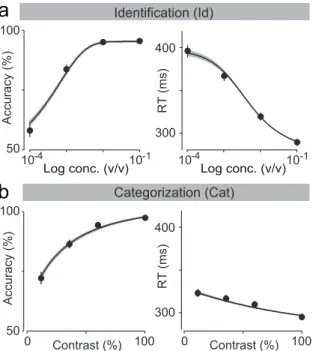
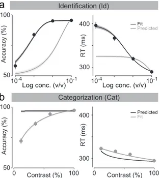
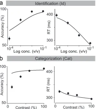
Figure 2.4. Comparison between odor identification and mixture catego-rization tasks. (a,b)Stimulus space in logarithmic scale for identification (a) and categorization (b) tasks. (c,d) Mean accuracy (c) and mean re-action time (d) for the identification task plotted as a function of odor concentration. (e,f ) Mean accuracy (e) and mean reaction time (f) for the categorization task plotted as a function of mixture contrast (i.e. the absolute percent difference between the two odors). Error bars are mean
± SEM over trials and rats. Dots are presented as to help parse between stimulus space and psych- and chrono-metric curves. Solid lines depict the obtained fits for RL-DDM model (Chapter 5).
2.4.2 Odor mixture identification task
Motivational variables can modulate performance and reaction time in perceptual tasks. For example, variables like reward rate (Drugowitsch, Moreno-Bote, Churchland, Shadlen, & Pouget, 2012) or emphasis for accu-racy vs. speed (Palmer et al., 2005; Hanks et al., 2006) can have an effect on observed SATs, by modulating decision criteria. Because identification and categorization tasks were run in separate sessions, we also consid-ered the possibility that rats might shift their decision criteria between tasks. To address this, and to cover the stimulus space more thoroughly, we devised a “mixture identification” task in which we interleaved the full set of stimuli from the categorization and identification tasks as well as intermediate mixtures. Thus, on each trial the stimulus was chosen ran-domly from one of four mixture ratios at one of four concentrations (Figure 2.5a). Consistent with the previous observations, RTs in this joint task were strongly affected by concentration but not by mixture contrast (Fig-ure 2.5b-c). A two-way ANOVA showed that OSD changed significantly across the different odorant concentrations (F(3,48) = 18.57, P <10−7); but for a given total concentration of the odorants, this change was not sig-nificant across the different mixture contrasts (F(3,48) = 1.61,P = 0.2). There was no significant interaction of odorant concentration and mixture contrast (F(9,48) = 0.20,P >0.9).
100 10-4 Odor A 10-1
Log conc. (v/v) 10-1
10-4
L
o
g
co
n
c.
(v/
v)
O
d
o
r
B
50 100
Accu
ra
cy
(%
)
0 100
Contrast (%) Contrast (%) 300
400
R
T
(ms)
0
a
b
c
Figure 2.5. Odor mixture identification task. (a) Stimulus design. Two odorants (S-(+)-2-octanol and R-(-)-2-octanol) were presented at differ-ent concdiffer-entrations and in differdiffer-ent ratios as indicated by dot positions. In each session, four different mixture pairs (i.e. a mixture of specific ratio and concentration and its complementary ratio) were pseudo-randomly selected from the total set of 32 mixture pairs and presented in an inter-leaved fashion. (b, c) Mean accuracy (b) and mean of reaction times (c) plotted as a function of mixture contrast. Each point represents a single mixture ratio. Error bars are mean±SEM over trials and rats. Solid lines are predictions from the RL-DDM model (Chapter 5), with shades repre-senting the 95% confidence interval simulated for the observed number of trials in the behavioral data. Colors represent the total concentration of the mixture, with black indicating a 10−1 mixture and lightest grey 10−4
Chapter 3
Noise and uncertainty in
olfactory decisions
“The cake is a lie”
3.1
Chapter Summary
In the previous Chapter we showed that, for a similar level of difficulty, identifying odors at low concentrations requires a much larger increase in stimulus sampling time than does discriminating similar mixtures, even when species, modality and motivation are controlled for.
In this Chapter, by taking a modeling approach, we investigate the role of sensory uncertainty in RTs and response accuracy observed in both identification and categorization task. We also address the possibility of additional sources of noise. This Chapter is divided in 3 sections:
• Introduction – a brief introduction regarding sensory uncertainty and accumulator models, in particular the drift-diffusion model.
• Sensory noise and the diffusion-to-bound model – in which
we explain our model implementation, the data fitting procedures and model comparison methods. We also present the obtained fits for our behavioral data and expose the challenge of fitting both tasks simultaneously.
• Additional sources of noise– where we address the DDM’s lack