* Corresponding author Tel.: +1-860-832-1824; fax: +1-860-832-1806 E-mail: [email protected] (H. Wang)
© 2012 Growing Science Ltd. All rights reserved. doi: 10.5267/j.ijiec.2011.08.019
International Journal of Industrial Engineering Computations 3 (2012) 81–92
Contents lists available at GrowingScience
International Journal of Industrial Engineering Computations
homepage: www.GrowingScience.com/ijiec
A scheme for functional tolerancing: A product family in 3D CAD system
Haoyu Wang* and Ravindra Thamma
Central Connecticut State University, New Britain, CT 06050 USA
A R T I C L E I N F O A B S T R A C T
Article history: Received 1 August 2011 Available online 10 August 2011
To meet the need for product variety, many companies are shifting from a mass-production mode to mass customization, which demands quick response to the needs of individual customers with high quality and low costs. The multifunctional nature of mechanical components necessitates that a designer redesign them each time when a component’s function changes. The functional Geometric Dimensioning & Tolerancing (GD&T) specification, also called functional tolerancing, must be updated for each component. Currently, this is done by humans, and thus can be very time-consuming and error-prone. Functional tolerancing is one of the main obstacles to practical mechanical product family modeling. In this paper, a graph-based functional tolerancing scheme in 3D CAD is proposed. In the scheme, a product is generated by applying production rules to the graph of the base product, following customers’ or manufacturing engineers’ requirements. Functional tolerancing of each component of a product in the family is formulated as a non-linear constrained optimization (or cost minimization) process. Certain critical aspects of the scheme
have been implemented in SolidWorks®, by using its Application Programming
Interface (API) and C++. LEDA® and MATLAB® have been used to solve the graph
and optimization problems.
© 2012 Growing Science Ltd. All rights reserved
Keywords: Tolerancing Product family Graph CAD
1. Introduction
mechanical product, about 75% of the final cost is determined in the product design stage. Therefore, design tools are highly demanded to help designers face the challenge of mass customization. Currently, there is no well-defined design process for developing a family of mechanical products, nor is there research work to support designers when a variant product in the same product family is generated. In addition, when detailed design of a component is finished, there is no support for designers to specify geometric tolerances.
Tolerance specification is the topic that has been least studied so far. It usually involves a series of activities, such as identifying features to be toleranced and the required datum features, determining types of tolerances needed and material conditions, and finally, assigning some of the tolerance values as per functional requirement. Other tolerance values should be generated in the tolerance synthesis process. Traditionally, these activities heavily rely on the designer’s experience, the empirical data, and/or the handbooks for designers and machinists. A systematic method is needed to automate this whole procedure, preferable in a CAD environment, incorporating domain-specific knowledge.
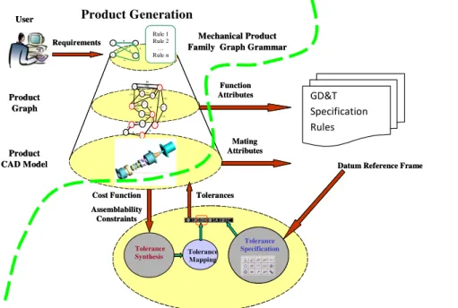
Fig. 1. Map of the scheme
In this paper, a graph grammar-based mechanical assembly family model is introduced. The generation of an assembly in the same family is modeled as the manipulation to the graph that represents the base assembly by applying graph production rules. The generated assembly variant is a graph with components as nodes and joints between components as edges. The joint information between components as well as the feature information of each component can help the designer in component design and tolerance specification. Fig. 1 illustrates the map of the overall scheme of the research in this paper. The research of this paper can be separated into two parts: mechanical product variant generation (product design) and tolerance generation (tolerance design).
In mechanical product variant generation, the user (a customer or a manufacturing engineer) enters his/her selections from a list of predefined requirements. The requirement selections are then mapped to the application conditions of a set of production rules. The production rules whose application conditions are satisfied are fired. The base product, which is represented by the graph of the product’s mechanism, is manipulated by the fired production rules. The customized product variant of the mechanical product family, which is also represented as a graph, is then generated after all the fired production rules are applied.
Rule 1 Rule 2 … Rule n 2 5 7 12 3 1
11
4
12 6 9 10 1 9 82 G G CYC PC HF HF F
F
CYI HF HF CYI CYC CYI CYI CYI CYI F
Figure 3.6.6 -2 Assembly graph of a planetary gearbox design PC PC PC PC Tolerance Mapping Tolerance Specification Tolerance Synthesis Product Graph Product CAD Model
Mechanical Product Family Graph Grammar User G 1 4 2
31
R
R
R G Function Attributes Mating Attributes Requirements
Datum Reference Frame
Cost Function Assemblability Constraints Tolerances Rule 1 Rule 2 … Rule n 2 5 7 12 3 1
11
4
12 6 9 10 1 9 82 G G CYC PC HF HF F
F
CYI HF HF CYI CYC CYI CYI CYI CYI F
Figure 3.6.6 -2 Assembly graph of a planetary gearbox design PC PC PC PC Tolerance Mapping Tolerance Specification Tolerance
Synthesis Tolerance Mapping
Tolerance Specification Tolerance
Synthesis Tolerance Mapping
Tolerance Specification Tolerance Specification Tolerance Synthesis Product Graph Product CAD Model
Mechanical Product Family Graph Grammar User G 1 4 2
31
R
R
R G Function Attributes Mating Attributes Requirements
Datum Reference Frame
Cost Function Assemblability Constraints Tolerances Product Generation GD&T Specification
Rules Tolerance Gener
ati
on
The graphs that represent the base product and product variants are attributed graphs. The attributes of nodes and edges of the graph are to carry quantitative or qualitative design information. The information is utilized in tolerance generation for tolerancing of each component in the product. The GD&T specification rules are followed to generate Datum Reference Frames (DRFs) on each component. Other features on the component are toleranced to the DRFs, and the tolerance types and material conditions are generated based on the attributes of the features. Tolerance values or ranges of tolerance values are obtained through tolerance synthesis and tolerance mapping.
2. Review
In the past two to three decades, design methods were continuously being developed, tested, implemented in industry, and taught to the engineering community. Customer needs are first transformed to a repeatable functional representation, then to layouts and solution pieces, then to broad combinations and alternative products, and finally to an embodied realization that we can produce for the customer.
The need in the market for product variety requires formal design process to develop a family of products instead of single products. Characteristics of a product family range from flexible modular designs to robust and scalable designs, to standardized and flexible products. Martin and Ishii (1996) identified commonality, modularity, and standardization; Rothwell and Gardiner (1990) emphasized robust design; Wheelwright and Clark (1992) suggested designing “platform projects” that were capable of meeting the needs of a core group of customers but were easily modified into derivatives through addition, substitution, and removal of features. MacDuffie et al. (1996) looked at how the variety affected manufacturing within the automotive industry by studying empirical data.
Geometry and tolerance requirement of a specific mechanical component may change from one product to another in the same product family. A well-defined mechanical product family model should provide the logical relationships between components. These relationships are very important for component designing and tolerancing. However, none of the methods mentioned above has taken this issue into account. In this work, a graph grammar–based mechanical product family modeling method is presented to generate variants in a product family with the joints between components updated for tolerance specification.
3. Graph-based Representation of an Assembly
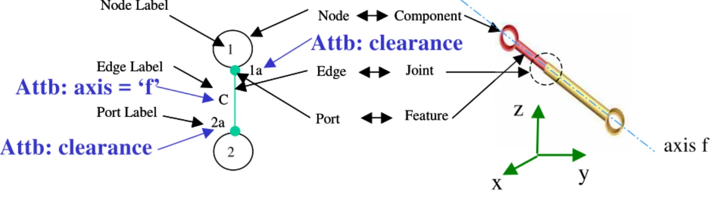
Figure 2 shows an example of the graph formalism of the graph of a piston assembly, where the bigger circles represent nodes (components), the smaller circles represent ports (features) of the nodes, and the lines between ports are edges (joints). Labels and attributes of nodes, edges, and ports are also illustrated.
Fig. 2. Graph representation of a piston assembly
3.1 Graph grammar of a mechanical product family
The term “graph grammar” generally means a method for generating a set of graphs from a starting graph. Manipulations on the starting graph are carried out by applying production rules. All graphs that can be derived by applying production rules to a starting graph construct the language of this graph grammar. This research adopts graph grammars as tools to model a mechanical product family. The strategy of graph grammar–based mechanical product family modeling is to design graph grammars to represent the organization of mechanical product family elements and accordingly to transform the variant derivation process into a process of assembly graph derivation.
Graph grammar with ordered production rules is called programmed graph grammar. In a programmed graph grammar, the sequence of executing a set of productions can be expressed in a control diagram. Product variants of the family can be derived by applying production rules according to the control diagram to modify the starting graph which represents the base product. The resultant graphs are the graph models of desired variants.
A Programmed Attributed Graph Grammar (PAGG) is defined as a nine-tuple:
GG = (V, W, X, AV, AW, AX, S, P, CD)
where V = {Ci} is a set, consisting of node labels (i.e., names or IDs) of all components in the product family; W = {Ci×Cj} is a set, consisting of edge labels that indicate the joints between the components; X is a set, consisting of port labels that represent features; AV is a set, consisting of node attributes representing attributes of components; AW is a set, including edge attributes representing attributes of joints; AX is a set, consisting of port attributes; S is the starting graph representing the base product; P = {pi} is a set, including all production rules defined for graph manipulation to generate variants; and CD is the control diagram over P, specifying the order by which productions are applied so that the variants can be derived.
All attributed graphs that can be derived by graph grammar GG as defined above are termed language of the graph grammar. The derivation steps are: 1) starting with a starting graph S; 2) applying all applicable productions P in an order specified by the control diagram CD.
1
2
Node
Edge
Port
Component
Joint
Feature C
Node Label
Edge Label 1a
2a Port Label
1
2
Node
Edge
Port
Component
Joint
Feature C
Node Label
Edge Label 1a
2a Port Label
axis f
Attb: clearance
Attb: clearance
Attb: axis = ‘f’
x
y
Set V in GG represents component names in a mechanical product family. It changes from family to family. Hence, it is trivial to list all possible component names. Component attributes AV may include parameters such as list of features, material, etc.
1) The Base Product
The base product should include common components or core components that all products in the same family contain. Other components in the same product family are termed optional components. The core components together with joints between them should fulfill common functions of the products in the family. Graph representations of a range of planar linkages, planar geared mechanisms, planar cam mechanisms, spherical mechanisms, and spatial mechanisms have been developed and cataloged in a graph atlas (Tsai 2001). The functional scheme and its graph representation of a crank-slider mechanism are shown in Figure 3. The circle enclosing the node indicates that the node is “grounded” or “fixed.”
Fig. 3. Crank-Slider mechanism and its graph representation
2)Production Rules
A production rule P has two parts: the operation (O) and its application conditions (π). The operation O = (gl, gr, T, P) designates how the left-hand side (LHS) graph, gl, is replaced by the right-hand side (RHS) graph, gr, with respect to embedding transformation, denoted by T, or port transformation, denoted by P.
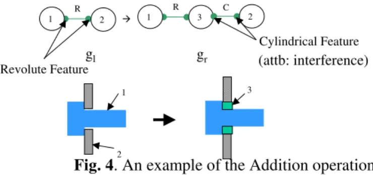
Addition
A particular component carrying out certain additional functions can be added to a base product to create a new product variant. Adding a component or subassembly C to a base product BP is equivalent to adding the graph g(C) to the host graph g(BP). Addition operation can be represented by a four-tuple: Addition = (gl, gr, T, P):
where gl is the conditional graph which implies that the base product provides interface for component C to be added; gr is the resultant graph after component C being added; and T is the embedding transformation function that specifies that all the edges connected to the components in gl will be connected to the corresponding components in gr.
2 R 1
R
1 3 2
Æ
C
gl gr
Revolute Feature
Cylindrical Feature
2
1 3
(attb: interference)
Decomposition
This category of operations serves the purpose of resembling the subsequent splitting of components into components that have simpler shapes. This kind of operation may be required by manufacturing or assembly practices. This category shows similar expressions to those in the “addition” category, with the slight difference that the created nodes here only serve part of the functions (joints with other components) of the original components. Decomposition operation can be represented by a four-tuple: Decomposition = (gl, gr, T, P), similar to the “addition” operation. An example of the Decomposition operation is shown in Fig. 5. In the example, component 1 is decomposed into the modified component 1 and component 3, so that the cylindrical feature mating with the gear (component 2) is transformed from the original component 1 to the component 3. This might happen when a component with many functional features is easier or more economical to be manufactured if it can be decomposed into several components.
Modification
Operations belonging to this category are intended not to extend the graph model obtained so far by adding nodes but rather to perform necessary modifications concerning the ports and attributes of nodes or relations among nodes. This may happen when we want to replace a component with one that has similar functions. For example, a customer may want to change a gear with one gear feature into a gear with two gear
features to get a larger input/output ratio. This is shown in Figure 6. Modification operation also can be represented by a four-tuple as above: Modification = (gl, gr, T, P).
2 Æ 1
1
3
2 3
G G
G
G
gl gr
1 2 3
Fig. 6. An example of the Modification operation
Fig. 5. An example of the decomposition operation
1 R 2 Æ 1 3 R 2
Cylindrical Feature
gl gr
1
2
After defining the operations used to modify graphs for variety generation, conditions under which the operations can be performed have to be specified, that is, when components should be added, decomposed, or modified. Application conditions are introduced for this purpose. When application conditions are satisfied, the applicability predicate, π, is TRUE. Otherwise, π is FALSE. Application conditions can be expressed as functions of customers’ or manufacturing engineers’ selected requirements or requirement values. A production rule is defined as a two-tuple: P = (O, π), where 1)
O ∈ {Addition, Decomposition, Modification} is the operation; 2) π ∈ {TRUE, FALSE} is the
applicability predicate, which is a logic function of application conditions. A few examples of production rules are given as follows, where Ri indicates requirement i of the product.
P1 = (O=Addition (Bearing), AC = (α(R1) ∈ {TRUE}))
P2 = (O=Decomposition (Holder), AC = (α(R3) ∈ {step}))
where α is a function to get the value of the requirement Ri and λ is a function to get the name of the
requirement Ri.
λ (R1) = Minimize Friction, α(R1) ∈ {TRUE, FALSE}
λ (R3) = Ease Manufacturing, α(R3) ∈ {step, non-step}
3) Graph Derivation
Deriving a product variant may involve more than one step of modification of the base product. The process of modifying a base product to a customized one can be modeled as a series of graph derivations by executing certain production rules. The derivation of a graph, g’, from a graph, g, by means of a production, p, follows the following procedures:
1. Check whether gl is a subgraph in g, and check if the application condition is true. If both condition s are fulfilled, continue to step 2.
2. Substitute gl, including all incoming and outgoing edges, with the nodes and edges of gr.
3. Transform the embedding of gl in g into gr in g’.
4. Update the ports of nodes in gr.
4) Control Diagram
Usually, a number of productions will be involved in the process of graph derivation. The order for a collection of productions to be invoked is specified by the control diagram. The control diagram in the graph grammar of a product family expresses the order in which productions defined for this product family are to be executed. Our method is to go through this process by imitating a real designer’s design practice in three stages: 1) adding new components or modifying existing
P1 P2 P3 P4
P5 P6
P7
Stage 1) Stage 2) Stage 3)
components in the mechanism to fulfill a customer’s or an engineer’s functional requirements; 2) increasing performance of the product by adding components, such as gaskets or bearings; and 3) adding positioning or fastening components to secure the relative positioning of the components in the assembly.
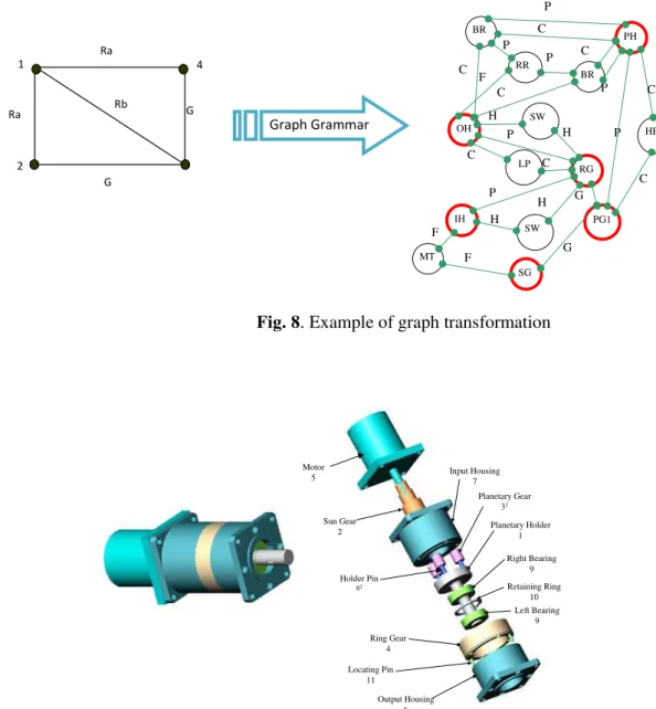
To map customers’ or manufacturing engineers’ requirements to a variant design, the checking of application conditions should start from the production that is at the beginning position of the control diagram. The path in the control diagram with the maximum number of applicable productions (application condition is TRUE) is chosen and all feasible productions along the path will be applied. A variant is generated when no more production rules in the path of the control diagram can be applied. Figure 7 shows an example of a control diagram. In figure 8, a graph that represents the base product of a planetary gear train is transformed into a graph that represents one possible product in the planetary gear train product family. Figure 9 shows the product’s physical model in SolidWorks®. For details of the graph generation process, please refer to Wang, 2005.
Fig. 8. Example of graph transformation
Fig. 9. CAD model of the planetary gearbox for the graph in Fig. 8
3.2 Functional tolerancing in 3D CAD
With enormous customer demands, commercial CAD systems open many more spaces for third-party developers to access the CAD model through API (Application Programming Interface) and develop
Input Housing 7
Planetary Gear 31
Sun Gear
2 Planetary Holder1
Left Bearing 9 Retaining Ring
10 Right Bearing
9
Ring Gear 4
Locating Pin 11
Output Housing 6 Holder Pin
82
Motor 5
Ra
Ra Rb
G
G 1
2
4
Graph Grammar
SG MT
IH
SW PG1 LP
RG SW OH
BR RR
PH BR
HPS
G G
C P
H F
F
C
H H
C C
C
C
C F
P P
P P
C
H P
software for their own use. In-house software can therefore be quickly prototyped and tested. SolidWorks has been chosen as the CAD platform to implement the proposed tolerance specification and tolerance synthesis methods owning to the following reasons:
• SolidWorks is a very popular CAD system based on a solid model which is 3D in nature. This matches our purpose for 3D tolerance specification and synthesis.
• The API is well documented.
• The API is easy to use and sample codes are available. • There is noo extra charge for the API.
The tolerance specification module and the tolerance synthesis module are developed as an add-in DLL (Dynamic Link Library) in SolidWorks by using the Object-Oriented Design method through SolidWorks’ API and MS Visual C++. The system structure is in Figure 10.
The user interacts with the tolerance specification module and tolerance synthesis module through SolidWorks Graphical User Interface (GUI) and GUI of the two modules by Microsoft Foundation Class (MFC).
3.3 Example
1)Tolerance Specification
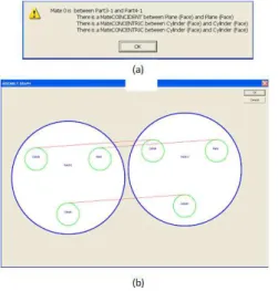
A base cover assembly is used to illustrate how the tolerance specification module and the tolerance synthesis module work in SolidWorks. The solid model of the assembly is shown in Figure 11. As can be seen, there are three mates between the Cover and the Base: a coincident mate between 1a and
Fig. 10. The structure of the implementation
User SolidWorks SolidWorks API
LEDA MatLab
Tolerance Specification
Tolerance Synthesis
Base
Cover
1a 2a 1b
2b 2c
1c
2a, a concentric mate between 1b and 2b, and a concentric mate between 1c and 2c. The tolerance specification module and tolerance synthesis module are programmed as an add-in to SolidWorks in Dynamic Link Library (DLL) file format. This add-in file can be loaded by opening the file directly in SolidWorks or by checking the respective check box in the Add-ins dialog box.
Tolerance Synthesis
In this paper, only features in mates are taken into account for tolerance synthesis to simplify the problem. The tolerance synthesis module shows mates between components and the connection graph as shown in Fig. 12. As shown in Fig. 13, three points are selected on each component for mating features. (37.5,20,0) is for T1a, T2a, and G1a/2a; (63, 20, 12.5) is for T1b, T2b, and G1b/2b; and (12, 20, 12.5) is for T1c, T2c, and G1c/2c. (0,0,0) is the origin of the base component (part 2) and is the point for T1; (0,25,0) is the origin of the cover component (part 2) and is the point for T2.
Fig. 12. Mates between components and the assembly graph Fig. 13. Spanning tree of the modified connection graph
Table 1-1 shows the labels of the nodes of torsors, their points’ coordinates, and LCSs. By using LEDA’s graph algorithm we get the spanning tree, as shown in Figure 13. Therefore, we know that there are only two independent loops: (Loop 1)1Æ1bÆ2bÆ2Æ2cÆ1cÆ1 and (Loop 2) 1Æ1aÆ2aÆ2Æ2bÆ1bÆ1. The two loops are represented by two rows of sequenced integers (0, 1, or –1) as shown in Table 1-2.
Table 1-1
Torsors’ labels, coordinates, and LCSs of the Cover-Base assembly
Node Label Torsor Coordinates (x,y,z) LCS (X-axis;Y-axis;Z-axis)
0
2
T (0,0,0) (1,0,0;0,1,0;0,0,1)
1
2a
T (37.5,20,0) (1,0,0;0,-1,0;0,0,-1)
2
2c
T (12,20,12.5) (1,0,0;0,-1,0;0,0,-1)
3
2b
T (0,25,0) (-1,0,0;0,1,0;0,0,-1)
4
1
T (63,20,12.5) (1,0,0;0,1,0;0,0,1)
5
1a
T (37.5,20,0) (1,0,0;0,1,0;0,0,1)
6
1c
T (12,20,12.5) (-1,0,0;0,-1,0;0,0,1)
7
1b
T (63,20,12.5) (1,0,0;0,1,0;0,0,1)
8
1 / 2a a
G (37.5,20,0) (1,0,0;0,1,0;0,0,1)
9
1 / 2c c
G (12,20,12.5) (-1,0,0;0,-1,0;0,0,1)
10
1 / 2b b
Table 1-2
Loop Matrix (note: N means node, L means loop)
N
L 0 1 2 3 4 5 6 7 8 9 10
1 -1 0 1 -1 1 0 -1 1 0 -1 1
2 -1 -1 0 1 1 1 0 -1 1 0 -1
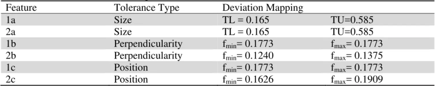
To solve the optimization (minimization) problem as formulated in this paper, the “fmincon” nonlinear constrained optimization solver in MATLAB is used. Results of the optimization run are shown in Table 1-3. The optimal deviation parameters are used for computing the tolerance values/ranges (Table 1-4).
Table 1-3
Optimal deviation parameters of torsors
Node dx dy dz Rx Ry rz
0 0.0099 0.01 0.0099 0.0017 0.0063 0.0005
1 -0.0001 0 0.01 0.01 0.01 0.0024
2 0.01 0.01 -0.0001 0.01 0.01 0.0011
3 0.01 0.01 0 0.01 -0.0028 0.0018
4 0.01 0.0099 0.01 0.0017 -0.0018 0.0015
5 0.0001 0 0.01 0.01 0.01 -0.0017
6 0.01 0.01 -0.0001 0.01 0.01 0
7 0.01 0.01 0 0.01 0.01 -0.0008
8 0.0001 0 0 0.01 -0.0028 -0.0017
9 0.01 0.01 -0.0001 -0.01 -0.0012 0.0001
10 0.0099 0.01 0 -0.01 -0.0036 -0.0008
Table 1-4
Results of tolerance values or ranges
Feature Tolerance Type Deviation Mapping
1a Size TL = 0.165 TU=0.585
2a Size TL = 0.165 TU=0.585
1b Perpendicularity fmin= 0.1773 fmax= 0.1773
2b Perpendicularity fmin= 0.1240 fmax= 0.1375
1c Position fmin= 0.1773 fmax= 0.1773
2c Position fmin= 0.1626 fmax= 0.1909
Table 1-4 listed the recommended ranges for size tolerances. But for perpendicularity and position tolerances, fmax and fmin values give the possible ranges of the values TU, TL, and Tp constrained by the mapping relations. These inequalities are planes in the TU, TL, Tp space and all such inequalities for each feature define the tolerance zone (Wang, 2006).
4. Conclusions and future work
design the product as well as how to translate the design knowledge to production rules for the product family. As described in section three, the key elements of a graph grammar of a mechanical product family are: a starting graph which represents the mechanism of the product, production rules, and a control diagram. Developing the three elements might not be a problem for an expert (even if it might take him or her months), but it could be very challenging for a designer who has very limited knowledge about graphs, production rules, etc. In order to make the proposed scheme convenient and efficient for all kinds of users, a generic system for mechanical product family modeling should be developed. It should allow users to select and edit starting graphs. Production rules should be generated based on user input such as customers’ or manufacturing engineers’ requirements, changes of features on components due to said requirements, etc. Users should be able to generate or edit the control diagram by their knowledge of design sequence and the support of the system.
There are two interesting questions about production rules that might indicate the directions of future study. One is “How do we know the production rules of a mechanical product family are complete?” The other is “How do we know if the production rules are optimal?” A complete production rule set should be able to generate product variants that meet all possible combinations of requirements for a product family. It should also represent all possible changes of the product configuration due to one specific requirement. An optimal production rule set is a complete one that has the minimum number of production rules. Future research about criterias that help users in evaluating the completeness of the production rules is needed to help searching for the optimal product design.
References
Anselmetti, B., Thiebaut, F., & Mawussi, B. (2002). Functional Tolerancing Based on the Influence of Contacts. APSE 2002 Summer Topical Meeting on Tolerance Modeling and Analysis. Charlotte, North Carolina. CD ROM. 15-16 July 2002.
Clement, A., Valade C., & Rivière A. (1996). The TTRSs: 13 oriented constraints for dimensioning, tolerancing and inspection. Proceedings of the Advanced Mathematical Tools in Metrology III Conference. Berlin. September, 25-28.
Kandikjan, T., Shah, J.J., & Davidson, J.K. (2001). A mechanism for validating dimensioning and tolerancing schemes in CAD systems. Computer-Aided Design, 33, 721-737.
Linares, J. M. (2002). Synthesis of tolerancing by functional group. Journal of Manufacturing Systems, 21(4), 260-275.
MacDuffie, J. P., Sethuraman, K., & Fisher, M. L. (1996). Product Variety and Manufacturing
Performance: Evidence from the International Automotive Assembly Plant Study. Management
Science, 42, 350-369.
Martin, M. V., & Ishii, K. (1996). Design For Variety: A Methodology for understanding the Costs of product proliferation. ASME Design Engineering Technical Conferences, Irvine, CA. 96-DETC/DTM-1610.
Rothwell, R., & Gardiner, P. (1990). Robustness and Product Design Families, Design management: a handbook of issues and methods. Moakley. Cambridge, MA. Basil Blackwell Inc.
Wang, H., & Roy, U. (2005). A Graph-Based Method For Mechanical Product Family Modeling And Functional Tolerancing. The 31st Design Automation Conference, ASME IDETC/CIE.
Wang, H., Pramanik, N., Roy, U., Sudarsan, R., Sriram, R.D., Lyons, K.W. (2006). A Scheme for Mapping of Tolerance Specifications to Generalized Deviation Space for Use in Tolerance Synthesis and Analysis. IEEE Transactions on Automation Science and Engineering (T-ASE).
3(1), 81-91.
Wheelwright, S. C., & Clark, K. B. (1992). Revolutionizing Product Development: Quantum Leaps in Speed, Efficiency and Quality. New York, The Free Press.