Received: 30 September 2009; Revised: 14 October 2009; Accepted: 21 October 2009 Published online in Wiley Interscience
(www.interscience.wiley.com) DOI 10.1002/pca.1192
A New Method for the Improvement of Data
Production in Phytochemical Analysis
João Ponte-e-Sousa
a* and António Neto-Vaz
a,bABSTRACT:
Introduction – The use of the average analytical signal for the construction of curves by the least squares method (LSM) over the standard addition method (SAM) is widespread. It would be advantageous, however, to fi nd a way to avoid intermediary averages, which are known to be the cause of signifi cant increases in standard deviations (SD).
Objective – To develop a protocol that uses all gathered data to create curves by LSM over SAM. To use Excel® for the estima-tion of y = mx + b and R2 rather than using LSM equations for the SD of m, x and b.
Methodology – The level of lead (II) in the bark (cork) of Quercus suber Linnaeus was determined using diff erential pulse anodic stripping voltammetry (DPASV). Three current samples were taken for each of the four standard additions. These signals were combined for adjustment by LSM. The results were compared with those obtained after averaging the current for each addi-tion, and the expression of uncertainty in the measurements determined.
Results – The new method shows an expanded uncertainty of ± 0.3321 μg/g (nearly 1.42%). The diff erence between the results obtained by the new and the old method is 0.01 μg/g (23.41 and 23.40 μg/g). The limit of detection changed approximately from 4.8 to 4 μg/g and the relative SD approximately from 9 to 6%.
Conclusion – The absence of intermediary averages in curves improved the determination of lead (II) in cork by DPASV. Estimation of SD only with LSM equations produced results that were signifi cantly worse. The changes are large enough to transform an apparently internally non-validated procedure (repeatability for precision) into an internally validated pro-cedure. Copyright © 2009 John Wiley & Sons, Ltd.
Keywords: Voltammetry; standard addition method; least squares method; cork
* Correspondence to: J. Ponte-e-Sousa, Department of Chemistry, University of Évora, Rua Romão Ramalho no. 59, 7000-671 Évora, Portugal. E-mail: [email protected]
a Department of Chemistry, University of Évora, Rua Romão Ramalho no. 59,
7000-671 Évora, Portugal
b ICAM (Institute for Mediterranean Agricultural Sciences), Pólo da Mitra,
University of Évora, 7000-Évora, Portugal
Introduction
No doubt numbers play an important role in phytochemical analysis but ‘the fact remains that many highly competent scien-tists are woefully ignorant of even the most elementary statistical methods. It is even more astonishing that analytical chemists, who practise one of the most quantitative of all sciences, are no more immune than others to this dangerous, but entirely curable, affl iction’ (Miller and Miller, 1988).
Using averages in the middle of data analysis reduces the infor-mation extractable from a set of measures. Ideally only fi nal results should be shown as averages. The present paper shows how to combine measurements of an analytical signal in such a way that all possible fi nal results inferable from a data popula-tion, such as the one presented in this study, will not be neglected. The use of this particular case of combinatorial analysis is com-pared with the earlier method for the estimation of the lead content in cork from Quercus suber L. by diff erential pulse anodic stripping voltammetry (DPASV). The eff ect that the new method has on the uncertainty of the estimation is emphasised. The new method extracts more information from the chemical analysis. In fact, instead of using just the curve of mean values of the analyti-cal signals for each concentration, it uses rs curves, where r is the number of repetitions of the analytical signal per concentration and s is the number of diff erent concentration values. The curves correspond to all possible choices of one measurement for each concentration.
Experimental
Standards and chemicals
The supporting electrolyte solution, 0.1 M sodium chloride, was prepared by dissolving sodium chloride p.a. from Merck (Darmstadt, Hessen, Germany) in Milli-Q water; the 0.1 M nitric acid solution was obtained by dissolving nitric acid 65% p.a. (Merck) in Milli-Q water; the 1.1 × 10⁻² M
lead (II) stock solution was obtained by dissolving lead nitrate from Riedel (Seelze, Lower Saxony, Germany) in 0.01 M nitric acid; a standard solution of 1.1 × 10⁻⁵ M lead (II) was achieved by diluting the stock solution
appro-priately. The digester reagents used were: nitric acid 65% p.a. (Merck) and hydrogen peroxide 30% p/v p.a. from Panreac (Castellar del Vallés, Spain, Spain). The solutions were prepared daily.
Extraction and digestion of cork sample
The interior of the bark of cork-oak was granulated with a plastic granula-tor, and an aliquot (0.09 g) of the resulting bark powder was mixed with 2 mL nitric acid and 0.25 mL of hydrogen peroxide. Following incubation for 2 h, the mixture was digested in a closed recipient at 85–90°C for 8 h.
DPASV analysis
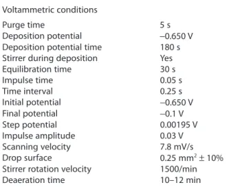
The instrumentation used for DPASV comprised an Eco Chemie Autolab/ pgstat 20 (Metrohm, Utrecht, Netherlands) potentiostat/galvanostat and a Metrohm VA stand 663 together with a hanging mercury drop electrode (HMDE), a glassy-carbon rod counter-electrode and an Ag–AgCl–KCl 3 M reference electrode. Eco Chemie GPES 4.9 software was employed to run the instruments and to obtain voltammograms. Voltammetric conditions were as shown in Table 1. For the voltammetric experiments, aliquots (0.1 mL) of the standard were added to 1 mL of the cork solution and 20 mL of the supporting electrolyte. Each measurement was made three times in each addition. Two-dimensional data treatment of current vs standard concentration was performed with the Excel 2003® line adjust-ment tool.
the blank assay, as usually employed to subtract any infl uence arising from all the solutions used for the correct treatment of the sample. The focus of this study is the random dependent variable i and four populations of three individual values resulting from the four standard concentrations tested are considered.
Old algorithm: least squares equations
Cork solutions. In order to show any existing diff erences in the
fi nal results, previous methodologies have been compared with the new methodology proposed here. As an example, focus will be given to the experimental results obtained for cork as shown in Table 2. Three current measurements are registered for each standard concentration. The electrolytic cell only contained dis-solved cork and supporting electrolyte when the fi rst recording was performed. A new HMDE (drop 2) subsequently replaced the old one, which had fallen into the cell. The same occurred after i had been recorded for drop 2. Thus, three consecutive recordings were obtained for each of the four standard concentrations, as indicated in Table 2.
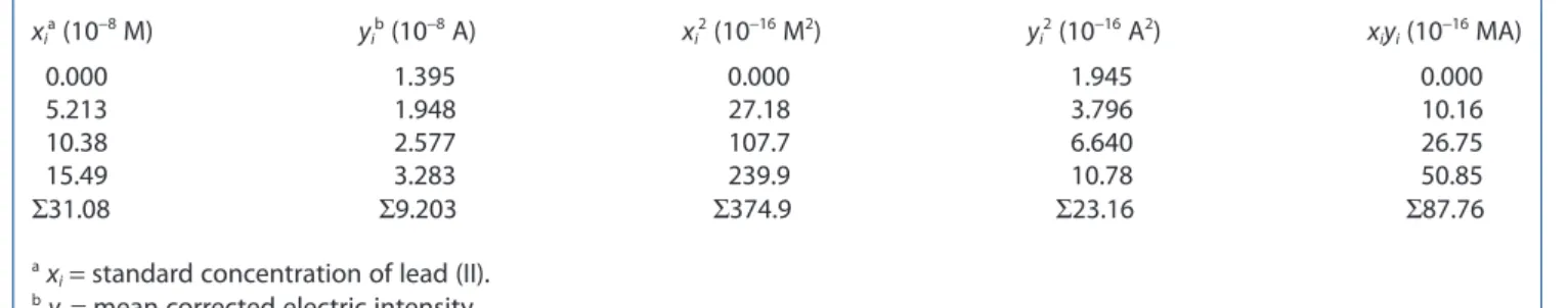
The fi rst comment is related to the initial step of the treatment of experimental results because LSM equations are usually applied after the reduction of all analytical signal recordings to their average values so that the LSM adjustments can be per-formed on a set of pair values, namely, analytical signal vs stan-dard concentration. Table 3 shows the average values for cork and successive calculations for the production of the necessary data for the least squares treatment.
The quantities Sxx, Syy and Sxy are needed to obtain all results allowed by LSM, where S x x N S y y N S x y x y N xx i i yy i i xy i i i i = −( ) = −( ) =ΣΣ −ΣΣ Σ Σ Σ 2 2 2 2 , , and
N being the number of data pairs used in the construction of
the curves. Substitution gives: S S S xx yy xy = × = × = × − − − 133 3 10 1 986 10 16 25 16 2 16 2 . , . , . . M A and 1016MA
Now the slope (m) of the adjusted line can be calculated as:
m=Sxy Sxx,from whichm=0 122. A M.
The intercept (b) with the analytical signal axis is:
b=Σy N m x Ni − Σ i ,from whichb=1 354 10. × −8A.
Table 1. Voltammetric conditions employed in the study
Voltammetric conditions
Purge time 5 s
Deposition potential −0.650 V
Deposition potential time 180 s
Stirrer during deposition Yes
Equilibration time 30 s Impulse time 0.05 s Time interval 0.25 s Initial potential −0.650 V Final potential −0.1 V Step potential 0.00195 V Impulse amplitude 0.03 V Scanning velocity 7.8 mV/s Drop surface 0.25 mm2± 10%
Stirrer rotation velocity 1500/min
Deaeration time 10–12 min
Table 2. Current measured by DPASV for the null, fi rst, second and third standard additions
Lead (II) concentration (10−8 M) Electric intensity i (10−8 A)
Cork Blank
0.000 1.463 1.349 1.372 0.780 0.774 0.769
5.213 1.932 1.961 1.952 4.063 4.069 4.069
10.38 2.564 2.624 2.543 7.016 7.052 7.178
15.49 3.323 3.237 3.289 9.880 10.22 9.950
Results and Discussion
Experimental measurements of the corrected electric intensity (i) produced an array of values that will be used as examples in the discussion in order to demonstrate their full exploitation. Table 2 shows i values measured three times for each of the four standard concentrations. Measurements reported refer to the sample material (a portion of the interior of the bark of cork-oak) and to
The standard deviation sy of the residuals is:
sy=
[
(
Syy−m S2 xx)
(N−2)]
,from which sy=5 830 10. × −10A.The standard deviation (sm) of the slope (m) is:
sm=sy Sxx,from which sm=5 049 10. × −3A M.
The standard deviation (sb) of the intercept (b) with the analyti-cal signal axis is:
sb=sy ⎡⎣1
(
N−( xi) xi)
⎤⎦ sb=4 888 10× −2 2 10
Σ Σ ,from which . A.
The equation for the least squares line is:
y=mx b+ ,from which y=(0 122. A M)x+1 354 10. × −8A.
The coeffi cient of determination (R2) is:
R2 x yi i xi y Ni xi xi N yi yi N
2 2 2 2 2
=(Σ −Σ Σ )
{
⎡⎣Σ −(Σ ) ⎤⎦⎡⎣Σ −(Σ ) ⎤⎦}
which, after appropriate substitution, gives R2 = 0.997.
Final Pb (II) concentration in electrolytic cell result appears, according to the standard addition method, as
0=(0 122. A M)x+1 354 10. × −8A↔ =x 1 111 10. × −7M.
The standard deviation (sc) for the analytical results obtained with the standard addition method is given by (Miller and Miller, 1988): sc=
(
s my)
⎡⎣( N)+( y Ni )(
Sxx)
⎤⎦ sc = × − 1 8 181 10 2 2 9 Σ m from which M , . .. sc=(
s my)
⎡⎣( )1L +(1N)+(yc− y Ni )(
Sxx)
⎤⎦ 2 2 Σ m is theequ-ation for the standard deviequ-ation of the analyte estimate for a cali-bration curve. In the case presented, yc equals zero, since the result stems from the intercept of the adjusted line with the hori-zontal axis, and L, the number of replicate measures of the sample, appears as infi nite, as if by extrapolating the adjusted line, thus making 1/L equal to zero.
Blank solutions. Table 4 shows averages for the blank and
suc-cessive calculations for the least squares treatment. The quanti-ties Sxx, Syy, Sxy that are required for LSM may be calculated in a manner analogous to that outlined above to give the following values: Sxx=133 3 10. × −16M2 Syy=47 29 10. × −16A2 Sxy=79 38 10. × −16MA m= 0 595. A M b=8 584 10. × −9A sy=10 97 10. × −10A sm=9 497 10. × −3A M sb=9 194 10. × −10A.
The equation for the least squares line is thus y = (0.595 A/M)x + 8.584 × 10⁻⁹ A, and R2= 0.999. The fi nal Pb (II) concentration in Table 3. Data obtained from cork solutions using the least squares method
xia (10−8 M) yib (10−8 A) xi2 (10−16 M2) yi2 (10−16 A2) xiyi (10−16 MA) 0.000 1.395 0.000 1.945 0.000 5.213 1.948 27.18 3.796 10.16 10.38 2.577 107.7 6.640 26.75 15.49 3.283 239.9 10.78 50.85 Σ31.08 Σ9.203 Σ374.9 Σ23.16 Σ87.76 a x
i= standard concentration of lead (II).
b y
i= mean corrected electric intensity.
Table 4. Data obtained from the blank using the least squares method
xia (10−8 M) yib (10−8 A) xi2 (10−16 M2) yi2 (10−16 A2) xiyi (10−16 MA) 0.000 0.774 0.000 0.600 0.000 5.213 4.067 27.18 16.54 21.20 10.38 7.082 107.7 50.15 73.51 15.49 10.01 239.9 100.3 155.2 Σ31.08 Σ21.94 Σ374.9 Σ167.6 Σ249.9 a x
i= standard concentration of lead (II).
b y
the electrolytic cell result appears, according to the standard addition method, as
0=(0 595. A M)x+8 584 10. × −9A↔ =x 1 442 10. × −8M,
and the standard deviation (sc) for the analytical results obtained with the standard addition method is sc = 1.734 × 10⁻⁹ M.
New algorithm
Linear regression, as performed using Excel 2003®, is a fairly easy way to treat data from the standard addition method, and is used in laboratories throughout the world. Nevertheless, the Excel® package used to execute these calculations has no way of directly attaining SD for the slope, yy intercept and x estimates, hence the need to develop an alternative way of obtaining such values. One can see that, in order to obtain such estimates, several slopes, yy intercepts and x estimates are needed. However, the question remains how to attain these values with data from one sample. The problem was solved using all available data instead of just the i means for each concentration. The corrected electric current, compensated for dilution eff ects, was used.
The fi rst step for the resolution of the problem was to verify whether every measurement was equally likely because none of them diff er much from the others. That is why any combination of four values for y, each stemming from its group of three repli-cates, should produce an adjusted line as favourable as the one resulting from its averages.
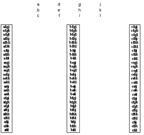
The data set, composed of three replicates of the corrected electric intensity for each of the four standard concentrations, can be combined in 81 diff erent ways (34). This is shown in
Fig. 1, where a, b and c are current measurements for the null addition, d, e and f are current measurements for the fi rst addi-tion, g, h and i are current measurements for the second addition and j, k and l are current measurements for the third addition. Tables 5 and 6 show these values, organised in the same order of the fi rst matrix of Fig. 1, respectively, for the cork solution and for the blank. This algorithm shows all possible combinations of values able to adjust a line by LSM, without repetition or change of column in such a way that all lines will be diff erent and will point to a diff erent estimate of the lead (II) content of the cork sample after blank subtraction. The algorithm is absolutely general and expresses itself as rs fi nal equations, r being the number of repetitions of the measurement of the analytical signal and s the number of standard additions, including the null addition.
The substitution of each letter in the matrix at the top of Fig. 1 by the numbers inside Tables 5 or 6, written in the same relative position, followed by the routine described in Fig. 1, will produce 81 sets of four i values, which will be the dependent random variable in each of the 81 graphs. The independent vari-able will be the concentration, which takes the values 0.000, 5.213, 10.38 and 15.49 × 10⁻⁸ M, as previously presented.
It is possible to write all 81 equations for the cork solution and the blank according to the combinatory scheme in Fig. 1, starting from the data inside Table 5 or 6, to which the scheme presented
Figure 1. The method used to obtain 81 regression lines (34
). The columns shown in the fi rst matrix are the corrected electric intensities measured for each of the four concentrations measured. The fi rst column is for the null addition, the second column is for the fi rst addition, the third column is for the second addition and the fourth column is for the third addition. By choosing one measurement from each concentration (i.e. one value from each column), a particular four-point data set for adjusting the corresponding regression line is obtained. There are 81 ways (which are listed in the three boxes) of constructing these four-point data sets.
Table 5. Cork i data positioned as in the fi rst matrix of
Fig. 1
Cork, i (10−8 A)
Addition 0 Addition 1 Addition 2 Addition 3
1.463 1.932 2.564 3.323
1.349 1.961 2.624 3.237
1.372 1.952 2.543 3.289
Table 6. Blank i data positioned as in fi rst matrix of Fig. 1
Blank, i (10−8 A)
Addition 0 Addition 1 Addition 2 Addition 3
0.780 4.063 7.016 9.880
0.774 4.069 7.052 10.22
0.769 4.069 7.178 9.950
in Fig. 1 is applied. Standard concentration sets are constant and are shown in the fi rst column of Table 2.
Several analytical parameters were determined from the 24 current intensities measured, as already presented, and the results are shown in Table 7. The main result is the fi nding of an expanded uncertainty (95% confi dence level) in the measure-ment according to ISO (1995) of U = 0.332 μg/g. Relative standard deviation falls from approximately 9 to 6%. Current data treat-ment allowed for the determination of the standard deviation of the coeffi cient of determination (R2), making the standard
devia-tion of R2 a new analytic parameter. It also allowed for the
estima-tion of a better limit of detecestima-tion, falling from approximately 4.7 μg/g to roughly 3.9 μg/g.
In this manner, the uncertainty measurement in lead (II) con-centration in cork can be measured using all available data instead of just the averages, which are unable to achieve the results presented here. Table 7 compares the values obtained using the new method presented in this paper with those from the older method.
In fact, one can see that, if all possible results from all data collected are treated, as has been done, their standard deviation is much smaller than the standard deviation predicted by least squares, and that the estimation of lead (II) concentration in the sample also diff ers (a diff erence of more than 0.01 μg/g was found in our case study).
Phytochemical analysis is of great importance throughout the world, particularly in the agro-industry, but quality certifi cation processes follow standard procedures that are not always fully understood by those who exercise them, thus making errors more likely to occur. The simplifi cation of approach is the best way to improve performance. In fact, the present approach was developed based on a serious doubt as to how to calculate stan-dard deviations of slope, xx and yy axis intercepts if least squares gave only one value for the slope and the xx and yy intercepts. It would require several measurements in order to calculate the averages and standard deviations. After all the equations for least squares are known (Miller and Miller, 1988), the knowledge of the foundations on which the estimation of those standard devia-tions is based would be complete. Nevertheless, if all least square
procedures commence by gauging the diff erences between y measured and y estimated, then the achievement of standard deviations should be possible through the study of all possible lines adjustable to experimentally measured yy data, specifi cally when it is possible to have a considerable number of repetitions of y values for each x value. The case studied above shows how to perform such an approach after three repetitions of each of the four y values, producing 81 lines. The variabilities of the slope and axis intercepts are revealed to be smaller than those esti-mated by least square equations, thus presenting a new way of estimating it which generates improved results.
The lead/cork case reported here can be used as a worthy model when alerting researchers to the possibility of signifi cant errors inherent in the addition of all experimental parameters. Although some of these parameters are not yet defi nable by hydrodynamics or electroanalytical chemistry, it is assumed that they are quasi-linear in their empirical use, but this clearly involves some risk in the fi nal result. The new method proposed warns of the need for a full understanding of the art of analytical science beyond the mere mechanical operation of equipment, with critical insight into the statistical procedure to be adopted for interpreting the results of the analysis of traces.
This method allows for the estimation of known analytical parameters after one single chemical analysis. The advantages of such an approach must be compared with its disadvantages; therefore this discussion will conclude with an enumeration of the main advantages and disadvantages.
The main advantage, and the underlying strength of the new approach, is to include all of the analytical signals. Methods are known for the elimination of extreme values, but there are no methods for the inclusion of coherent values in their absolute state, only their averages. In relation to the elimination of the extreme or incoherent values, one must refer to a criterion for the rejection of incoherent values: the Q test
assumes that the distribution of populational data is normal. [Nevertheless], this condition cannot be proven as true or false for distributions with less than 50 results. (. . .) This is why J. Mandel, talking about a small set of data, writes: “Those that believe that they can reject observations using an exclusion criterion integrated in a statistical rule for the rejection of incoherent values are just deluding themselves.” (. . .) In the end, the only valid reason for the rejection of a result within a small group of data is the knowledge that some mistake was done during the measuring. Without this knowledge it is advised a careful approximation to the exclusion of values of incoherent appearance [for that a statistical rule is just an important auxiliary]. (Skoog et al., 1988).
Using just the averages instead of all the information in the data set is also a process of exclusion but, contrary to the exclu-sion of outliers or incoherent data, it excludes quite coherent measurements. This clearly changes the fi nal result, mostly its uncertainty, as is shown in the above example, and must be avoided at all times. The simplest way to do this is through the application of the new method, which considers all analytical signal data equally.
Also relevant is the possibility of gauging the uncertainty of measuring of the analytical signal for each set of such measure-ments. In the above practical application, 24 signals were needed and an exact estimation of the expanded uncertainty related to the measuring of the analytical signal variable was achieved.
The present approach also allows for the estimate of a minimum value for total uncertainty in an analysis from only one
sample, as well as the characterisation of each analysis using several usual parameters estimated from a single sample. Since this approach does not need equations for the standard devia-tions of the slope and of the yy and xx axis intercepts, it can be implemented in Excel® much more easily using the line adjust-ment routines. Uncertainty can now be calculated.
Several disadvantages were, however, encountered: The fi rst is that, for a constant number of repetitions of the measurement of the analytical signal, the number of values increased exponen-tially with the number of concentrations used in the standardisa-tion process (a large number of values can therefore be achieved, even though this disadvantage is currently of little interest due
to the use of computers). This method using LSM is also inade-quate when any of the assumptions of the method are not ful-fi lled, speciful-fi cally when autocorrelation of the analytical signal appears. It is also very important to point out that the purpose of the method is to study a single sample. Using it to avoid the repetition of the measurement of as many samples as needed would be a real scientifi c disadvantage, even though the produc-tion of data that this new method permits can be used to simu-late a great number of sample repetitions.
It is well understood that t statistics are being used as if aver-aged fi nal concentration resulted from between 50 and 100 values (t = 2), which is true for the new but not for the older
Table 7. Analytical parameters
New algorithm Old algorithm
Cork Blank Cork Blank
m (A/M) avg 0.122 0.595 0.122 0.595 s 0.004 0.009 0.005 0.010 b avg (10−8A) 1.354 0.858 1.354 0.859 s (10−10A) 3.632 3.045 4.914 9.232 R2 avg 0.995 0.999 0.997 0.999 s 0.003 0.000 n.a.a n.a. [Pb (II)] avg (10−8 M) 11.13 1.443 11.12 1.444 s (10−10 M) 61.44 7.040 82.35 17.43 unb (10−10 M) 6.826 0.782 n.a. n.a. LOD (10−8 M) 1.654 (3.998 μg/g) 1.967 (4.755 μg/g) LOL (10−8 M) 15.49 15.49 CV (%) 5.521 4.879 7.403 12.07 N 81 1 [Pb (II)]t avg (10−8 M) 9.685 9.680 stc (10−10 M) 61.84 84.17 **U (10−10 M) 13.74 n.a. Dd 241.7 241.7 Cmasse (μg/g) avg 23.41 23.40 stc 1.495 2.035 CVs (%) 6.385 8.696 Ub 0.332 n.a. CVU (%) 1.419 n.a. Δ (μg/g) 0.013 Δr (%)f 0.000(1)
The line produced by the least squares method is applied to the standard addition method: b is the intercept with the yy axis, m is its slope (method sensitivity), R2 is the coeffi cient of determination, avg is the average, s is the absolute standard deviation, LOD
is the limit of detection, i.e. ‘blank plus three times standard deviation of the blank’ (Skoog and Leary, 1992), LOL is the limit of linearity and CV is the coeffi cient of variation, the ratio s/avg × 100 or U/avg × 100. Number of values (N) = 81 for each—cork and blank—for new algorithm and 1 for the old algorithm
a n.a. = not applicable.
b Partial uncertainty, u s n
n= n ; combined standard uncertainty, u=
(
u12+u22)
; expanded uncertainty, U = u × 2 (** confi dencelevel of 95%) (ISO, 1995).
cs s s
t=
(
cork2+ blank2)
.d 21 × 5 ml × 207.2 g/mol/0.09 g.
e Mass-based concentration [μg Pb (II)/g of cork (interior of the bark of Quercus suber L.)]. f Δ
approach. Nevertheless, the equation for the standard deviation of the estimated concentration by the standard addition method diff ers from that of the calibration curve because estimation pre-tends that an infi nite number of analytical signal measures were performed (1/L equals zero). This would lead to the logical con-clusion that uncertainty of the previous approach would be zero. The non-application of this conclusion is advised.
The new approach shows a diff erent result by including all current intensity measurements. The new approach does not use the least squares equation for the standard deviation of the results. This equation produces a standard deviation of the results based on points of the line that are not treated as averages (with their standard deviation), but simply as points of the line. That is why the older approach, in which the standard deviation of the result is based solely on the diff erences between the least square estimation of the points of the line and their averages, is shown as being poor for the production of a fi nal result. In the new method the standard deviation also uses the diff erences between original analytical signal measurements (resulting in their stan-dard deviations). In the end, repeatability of analytical signals measurement and its relevance to the precision of the estimate of the lead (II) concentration are the present work’s most important issues. All the results were presented with four signifi -cant digits, but the intermediary computations used as many digits as the Excel® allowed (30). Alternative ways to show how
standard deviations of medium points (used to construct an adjusted line) would aff ect the lead (II) concentration estimate were investigated.
Acknowledgements
Thanks are due to (chronological order): grant number SFRH/ BD/31420/2006 from the Foundation for Science and Technology of the Ministry of Science, Technology and Higher Education of Portugal; Russell Alpizar-Jara, from the Department of Mathematics, University of Évora; David Zellmer, from the Department of Chemistry, California State University, Fresno; Victor M. M. Lobo, from the Department of Chemistry, Univers-ity of Coimbra; Carlos Braumann, from the Department of Mathematics, University of Évora.
References
ISO, 1995. Guide to the Expression of Uncertainty in Measurements. International Standard Organization: Geneva.
Miller J, Miller J. 1988. Statistics for Analytical Chemistry. Ellis Horwood: Chichester.
Skoog DA, Leary JJ. 1992. Principles of Instrumental Analysis. Saunders College: New York.
Skoog D, West D, Holler F. 1988. Fundamentals of Analytical Chemistry. Saunders College: New York.