Universidade de Lisboa
Faculdade de Ciências
Departamento de Biologia Animal
Searching for an ecological
indicator based on plant functional
diversity along a climatic gradient
Dissertação
Melanie Köbel Batista
Mestrado em Ecologia e Gestão Ambiental
2013
Universidade de Lisboa
Faculdade de Ciências
Departamento de Biologia Animal
Searching for an ecological
indicator based on plant functional
diversity along a climatic gradient
Melanie Köbel Batista
Dissertação orientada por: Doutora Cristina Branquinho
Profª Doutora Otília Correia
Mestrado em Ecologia e Gestão Ambiental
2013
II
Agradecimentos
Obrigada ao meus pais por me permitirem fazer este mestrado e por, basicamente, estarem sempre lá.
Obrigada à Profª Cristina Branquinho por ter aceitado orientar-me, e por me ter literalmente orientado quando me sentia desorientada, por me ter motivado e permitido acreditar em mim própria. Muito brigada também pela atenção, cuidado e tempo que me dispensou!
Obrigada à Profª Dra. Otília Correia a orientação da tese, especialmente peos decisivos comentários finais que levaram a uma melhoria importante na tese e que me alertaram para importantes questões!
Agradeço também ao projecto “Modeling Ecosystem Structure and Functional Diversity as early-warning indicators of Desertification and Land-degradation - from regional to local level” PTDC/AAC-CLI/104913/2008 pelo apoio financeiro que permitiu a realização deste trabalho.
Obrigada à Susana que me acolheu tão bem, que teve a paciência de me ensinar a identificar plantas e que foi óptima companheira de saídas de campo. Obrigada também prontidão com que sempre me ajudas!
Grandessíssimo obrigada à Alice, pela sua paciência, simpatia e solidariedade com as minhas infindáveis dúvidas e pela atenção desmesurada que deu a esta tese na decisiva recta final. Alice, sem ti este tese não seria nem metade. Muito obrigada.
Obrigada Pedro, pela disponibilização de dados e pela prontidão em ajudar-me sempre que precisei.
Obrigada a todo o pessoal do ESFE que me acolheu tão bem, vocês fizeram-me sentir em casa!
Obrigada Ninda e Filipa pela simpatia e amizade, e pela ajuda no trabalho que mais ninguém tinha tempo de fazer…
Obrigada Andreia F., Andreia A., Adriana e Inês pela amizade. Sem ela não há vida possível. Um especial obrigado a ti Andreia, pelo companheirismo sem fim nas longas saídas de campo.
Obrigada à Giulia e ao Mauro pela pronta disponibilidade em ajudar nas saídas de campo. Eu sei, foi trabalho árduo…
Obrigada à minha querida mãe que tem a capacidade de me dar o empurrãozinho mesmo por telefone. Amo-te muito!
Obrigada ao B., por todos os dias lado-a-lado, por continuares ao meu lado mesmo nos meus dias maus, e mesmo quando esses dias se transformam em semanas ou meses.
Obrigada avô, tenho a certeza que, se hoje estou onde estou, se estou a fazer esta tese que estou a fazer, uma boa parte é por causa mundo maravilhoso que tu me mostraste. Danke. Ich werde dich nie vergessen. Wie könnte ich?
V
Abstract
Searching for early indicators of climate change is of utmost importance in drylands, since these regions are particularly sensitive to desertification, due to water scarcity and land-use impacts. Our main objective was to search for a potential ecological indicator of climate change. For that, plant community was assessed along a spatial climatic gradient in a dryland area located in southern Portugal. Plant community was assessed in 15 sites that varied in mean annual precipitation (521-634mm) and mean annual temperature (16-17°C), in Mediterranean grasslands. Plant community was studied both in a classical approach (species diversity and plant cover) and in a functional approach (through the analysis of several a priori functional groups and measured traits related to climate) and related to climatic variables. The point-line intercept method was used to assess plant community. A priori functional groups were based on life form, life cycle and families. Traits measured were biomass, height and SLA.
The sampled sites were dominated by annual grasses. Species richness and plant cover decreased significantly with increasing aridity. Considering a priori functional groups, the cover of hemicryptophytes decreased with increasing aridity, as well as cover of perennial grasses and annual legumes while cover of annual grasses remained unchanged. Along the climatic gradient, a community shift was found based on relative cover (relative % in the plant community): annual grasses and Plantaginaceae species increased their relative cover with increasing aridity, while perennial grasses, annual legumes and Caryophillaceae species decreased in relative cover. A multivariate analysis grouped species in a manner consistent with the previous result. Among a priori functional groups, the most promising groups with potential to be used as ecological indicators are perennial grasses and annual legumes and the previously mentioned community shift.
Biomass and height changed along the climatic gradient, although the response pattern found for dominant species did not always match the response of their respective a priori functional groups. For example while height of annual grasses increased with precipitation, height of the dominant annual grass A. pourretti did not significantly changed. Specific leaf area, which was analyzed only for the Compositae species Tolpis barbata, decreased with increasing aridity as well. Considering that the height of this species also decreased, this suggests a change in the physiological performance along the climatic gradient. Moreover it reflects the phenotypic plasticity of this species. In sum, the response of specific
VI
traits (e.g. height or SLA) measured in the same species along the gradient seems to have the potential to be used as an ecological indicator of climate change, especially in species with global distribution.
Key-words
VII
Resumo
As alterações climáticas podem ter consequências especialmente graves em zonas áridas, uma vez que a escassez de água aliada a pequenas alterações no clima ou na gestão do uso do solo podem gerar transformações abruptas e dificilmente reversíveis, comprometendo os serviços prestados pelos ecossistemas (MEA 2005). A produtividade nestas zonas já é limitada pela falta de água e, neste contexto, as alterações climáticas podem inclusivé induzir um processo de desertificação iminente (UNCCD 2011). Assim, a procura de indicadores ecológicos, i.e. parâmetros do ecossistema que reflictam a sua resposta a determinado factor ambiental (Turnhout et al. 2007), que permitam antecipar os efeitos das alterações climáticas é de extrema importância (MEA 2005).
As previsões climáticas para Portugal apontam para um decréscimo de precipitação ao longo do próximo século, especialmente acentuado na região sudoeste do país (Costa et al. 2012). Esta região tem atualmente valores de precipitação muito baixos (Rosário 2004) pelo que está classificada como zona árida, de acordo com classificação da Convenção das Nações Unidas para o Combate à Desertificação (MEA 2005), apresentando uma elevada variabilidade interanual (Soares et al. 2012). Estas características tornam-na uma zona susceptível a processos de desertificação que poderão ser acentuados pelas referidas previsões climáticas.
Atributos funcionais são características mensuráveis das plantas, relacionados com o seu funcionamento, modelando a forma como respondem a variáveis ambientais ou influenciam os processos do ecossistema (Lavorel et al. 2007a). A utilização de grupos funcionais – grupos de espécies com atributos semelhantes – é muito vantajosa pois além de fornecer informação sobre os processos dos ecossistemas, inacessível numa abordagem baseada na composição específica, foi também demonstrada a relação entre diversidade funcional e vários factores de perturbação tais como pastoreio, disponibilidade de nutrientes, fogo, etc. (Scherer-Lorenzen 2005, Lavorel et al. 2007a). Acresce que, ao contrário de uma
VIII
abordagem clássica baseada apenas na diversidade específica, esta permite comparar diferentes comunidades vegetais sob o ponto de vista funcional.
Neste trabalho, pretende-se encontrar um potencial indicador ecológico dos efeitos das alterações climáticas. Para isso, avaliou-se a comunidade vegetal ao longo de um gradiente climático, localizado em clima mediterrânico, usando quer uma abordagem específica, quer uma baseada na diversidade funcional. A comunidade vegetal foi avaliada ao longo de um gradiente climático espacial, no qual a precipitação média anual variou entre 521 e 634mm. Os 15 locais amostrados localizados em Montado de azinho são homogéneos relativamente a uma série de parâmetros (baixa intensidade de pastoreio, tipo de solo, altitude, pH, litologia e não ocorrência de fogo recente) e foram aleatoriamente selecionados após estratificação baseada na precipitação média anual dos últimos 50 anos.
A comunidade vegetal foi amostrada usando o método dos quadrados pontuais. As espécies encontradas foram classificadas em vários grupos funcionais definidos a priori, relacionados com a forma de vida, o ciclo de vida e a família taxonómica (como uma aproximação à classificação por grupos funcionais, uma vez que agrupam espécies que partilham uma série de características). Alguns atributos funcionais foram medidos: biomassa, altura vegetativa e área específica foliar. De uma forma geral, este estudo pretende responder às seguintes questões: i) a diversidade específica e a cobertura de plantas variam ao longo do gradiente?; ii) qual o padrão de resposta dos vários grupos funcionais?; iii) ocorrem mudanças ao nível da comunidade como um todo (em termos de cobertura relativa)?; iv) podem os atributos funcionais ser usados para avaliar gradientes climáticos, ao nível da espécie e ao nível da comunidade?; v) será possível identificar um limiar após o qual ocorram alterações significativas ou abruptas no ecossistema?; vi) quais são os caracteres ou grupos funcionais com maior potencial para se tornarem indicadores ecológicos de alterações climáticas? Uma vez que indicadores ecológicos devem ser parâmetros simples e de medição o
IX mais expedita possível, de modo a potenciar uma utilização a larga-escala, a estrutura deste trabalho segue uma linha de crescente especificidade nos parâmetros avaliados começando por parâmetros relativamente simples, nomeadamente diversidade específica e cobertura, seguida por uma avaliação ao nível do grupo funcional e terminando numa avaliação ao nível específico.
Considerando os 15 locais amostrados, foram identificadas ao todo 146 espécies, na qual a sua maioria pertence às famílias Graminae (37 espécies), Compositae (29) e Leguminosae (22). A cobertura de plantas foi, em média, ca. de 80%, dominada por gramíneas anuais, que ocupavam, em média, 51.8% da comunidade vegetal. A diversidade específica e cobertura de plantas aumentou significativamente com o aumento da aridez (i.e., ao longo do gradiente climático). No entanto, visto que estes parâmetros estão muito dependentes do clima e uso do solo, sugere-se que um indicador ecológico baseado na diversidade funcional será mais apropriado para uma aplicação a larga-escala. Considerando os grupos funcionais avaliados, os resultados mostraram que a cobertura de espécies hemicriptófitas diminuiu com o aumento da aridez, bem como a cobertura de gramíneas perenes e de leguminosas anuais, enquanto que a cobertura de gramíneas anuais permaneceu inalterada. Esta classificação que tem em conta conjuntamente a família e o ciclo de vida (ex. gramíneas perenes), mostrou ser mais eficaz do que os primeiros grupos funcionais avaliados, que têm em conta apenas um atributo (apenas forma de vida, por exemplo). Portanto, com base nestes resultados, os grupos que parecem ter maior potencial para se tornarem indicadores ecológicos das alterações climáticas são as gramíneas perenes e as leguminosas anuais. Estes resultados estão de acordo com vários estudos que associam gramíneas perenes e leguminosas a sítios mais húmidos.
Ao analisar a cobertura relativa (%) de locais em extremos opostos deste gradiente climático, verificou-se que, além dos grupos acima referidos, também outros taxa variavam a sua cobertura relativa. Verificou-se que 2 grandes grupos variavam inversamente: à medida que os locais são cada vez mais áridos, a
X
cobertura relativa de um grupo composto pelas gramíneas anuais e espécies Plantagináceas aumenta (de ca. 40% para 60%), enquanto que outro grupo composto pelas gramíneas perenes, leguminosas anuais e espécies Cariofiláceas diminui (de ca. de 30% para 10%). Uma vez que estes resultados são com base em grupos funcionais feitos a priori, foi também efetuada uma análise multivariada para verificar como as espécies se associavam entre si. Os resultados são consistentes com os grupos funcionais considerados. No entanto, também permitiu verificar que, dentro dos grupos funcionais, podem existir espécies que não mostram o mesmo padrão de resposta que o grupo funcional em que se esta insere, o que sugere que a comunidade vegetal deve continuar a ser analisada, de modo a refinar os grupos funcionais considerados.
A biomassa e a altura vegetativa são atributos funcionais que mostraram responder ao gradiente climático, embora a resposta varie entre os vários grupos funcionais e as espécies dominantes. A área específica foliar, medida para a espécie Tolpis barbata, diminuiu significativamente com o aumento da aridez. Considerando que a altura vegetativa desta espécie também decresceu, a resposta conjunta destes dois atributos funcionais sugere que há uma reposta fisiológica por parte da planta ao gradiente climático. Os resultados sugerem que a resposta destes atributos funcionais medidos na mesma espécie ao longo do gradiente, pode constituir um potencial indicador ecológico. No entanto, para que um indicador ecológico deste tipo seja aplicável em larga-escala, deve ser utilizado numa espécie com distribuição global.
Palavras-chave
atributos funcionais; diversidade funcional; Mediterrâneo; gradiente climático; pastagens
XII
Figure Index
Figure 1: Climate classification of Portugal based on the Aridity Index, using climatic data from years 1961-1999. Adapted from: Rosário (2004).
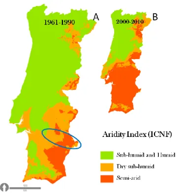
Figure 2: Climate classification of Portugal based on the Aridity Index. A: current official classification, using data from years 1961 to 1990; B: a provisional classification using data from decade 2000 to 2010. The sampling area is marked with a blue circle. Adapted from: (Rosário 2004).
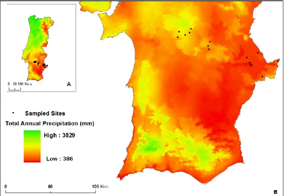
Figure 3: Maps of Portugal showing a precipitation gradient, based on total annual precipitation from years 1950-2010. A: Map of continental Portugal. B: Map of south Portugal, evidencing the sampled sites marked by dots. Maps constructed using data of Hijmans et al. (2005).
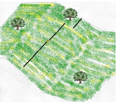
Figure 4: Exemplification of the disposition of the 6 transects in the field. The red point corresponds to the ICNF point, located using a GPS. The 6 transects are arranged perpendicularly to the slope and one transect is deviated to avoid a tree.
Figure 5: Sampling work. The method used for individuals collection consisted in a packaging system, where all hits of one point were packaged together and these small packs were grouped by transect and then by site for further identification and trait measurement in the lab.
Figure 6: Median, 25th and 75th percentiles, minimum and maximum, outliers and
extreme values of A: plant cover and no plant cover; B: percentage of bare soil, litter,
lichen and bryophyte within the no-plant points, in 15 sites sampled along a climatic gradient in Alentejo region.
Figure 7: Median, 25th and 75th percentiles, minimum and maximum value of number
of species, in all sites sampled (15 sites), along a climatic gradient in Alentejo region.
Figure 8: Median, 25th and 75th percentiles, minimum and maximum, outlier and
extreme values of A: number of species and B: relative cover percentage of herbaceous and shrub understory, in 15 sites sampled along a climatic gradient in Alentejo region.
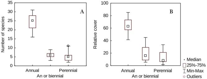
Figure 9: Median, 25th and 75th percentiles, minimum and maximum, and outlier
values of annual, facultative biennial and perennial herbaceous species in terms of A: number of species and B: relative cover in the community, in 15 sites sampled along a climatic gradient in Alentejo region.
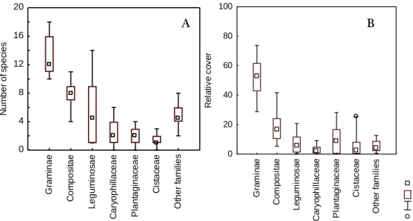
Figure 10: Median, 25th and 75th percentiles, minimum and maximum and
outliers values of community composition among the study sites regarding families, in terms of A: number of species and B: relative cover percentage.
Figure 11: Bi-plot of plant cover (grey quadrats) an no plant cover (black dots) with the aridity index (calculated with data from Y1960-1990).
XIII Figure 12: Bi-plots between measured number of species and A: minimum temperature of the coldest month (mean from Y1950-2000); B: short-term precipitation (mean monthly precipitation from Oct 2011 – Mar 2012). Plant community was sampled in 14 sites along a climatic gradient in Alentejo region.
Figure 13: Plant community composition of the more humid and the driest sites according to Medium-term Precipitation, i.e. mean annual precipitation from years 1998-2011 (MTPrec), using relative cover data of a sampling performed in 14 sites along a climatic gradient in Alentejo region.
Figure 14: Relative cover in the community of functional groups considered in table 12 along sites with increasing long-term precipitation (mean annual precipitation from period 1960-1999). Plant community was sampled in 14 sites along a climatic gradient in Alentejo region.
Figure 15: Non-metric Multivariate Dimensional Scaling (NMDS; first vs. second axes) of cover of the 21 most dominant species and sites. Distance measure used was Bray Curtis and stress was 0.097. Numbers indicate sites sorted in ascending order of long-term precipitation (as in Appendix 1). Simbols were placed manually on the left of the species name to indicate species assignment to functional group or family considered in previous results. Apour= Agrostis pourretii Willd.; Bdyst= Brachypodium distachyon (L.) P.Beauv.; Bhord= Bromus hordeaceus L.; Ccapi= Crepis capillaris (L.) Wallr.; Cdact= Cynodon dactylon (L.) Pers.; Cmixtu= Chamaemelum mixtum (L.) All; Crace= Carlina racemosa L.; Gfragi= Gaudinia fragilis (L.) P.Beauv.; Hglab; Hypochaeris glabra L.; Lgall= Logfia gallica (L.) Coss. & Germ.; Lrigi= Lolium rigidum Gaudin; Ltara= Leontodon taraxacoides (Vill.) Mérat; Ocomp= Ornithopus compressus L.; Pcoro= Plantago coronopus L.; Plago= Plantago lagopus L.; Spurp= Spergularia purpurea (Pers.) G.Don; ; Tbarba= Tolpis barbata (L.) Gaertn; Tgutt= Tuberaria gutatta (L.) Fourr.; Vcili= Vulpa ciliata Dumort.; Vgeni= Vulpia geniculata (L.) Link; Vmyur= Vulpia myuros (L.) C.C.Gmel..
Figure 16: Bi-plots between climatic variables and SLA (m2kg-1) of annual forb
Tolpis barbata sampled along a climatic gradient in Alentejo region. This species was present in 12 of the 14 sites sampled. A: relation of SLA with the aridity index (calculated using climatic data from Y1960-1990); B: relation of SLA with long-term precipitation (mean annual precipitation Y1950-2000).
XV
Table Index
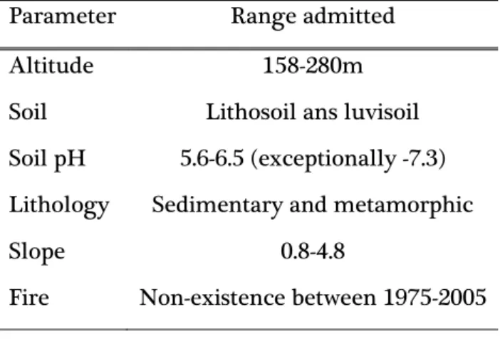
Table 1: Parameters used for homogenize the sampling sites.
Table 2: Climatic variables considered in this work. For each climatic variable is shown the abbreviation adopted, description, calculation and source.
Table 3: Number of species per family found in 15 sites sampled along a climatic gradient in Alentejo region.
Table 4: Spearman’s rank correlation coefficients at P<0.05 for no plant cover, percentage and standard deviation (SD), plant cover and species richness (Nr sp) of 14 sites sampled along a climatic gradient in Alentejo region. Ns= non-significant. Climatic variables: Arid. Idx= Aridity index (using data from Y1960-1990); LT Prec= long-term precipitation (mean annual precipitation Y1950-2000); MT Prec= medium-term precipitation (mean annual precipitation Y1998-2011); ST Prec= short-term precipitation (mean monthly precipitation Oct 2011 to Mar 2012); LT Temp= long-term temperature (mean annual temperature 2000); TColdM= minimum temperature of the coldest month (mean Y1950-2000).
Table 5: Traits compiled from the literature for the species present in the precipitation gradient. Traits analyzed are highlighted.
Table 6: Spearman’s rank correlation coefficients at P<0.05 for species richness, total cover and relative cover of functional groups based on life form. Climatic variables: Arid. Idx= Aridity index (using data from Y1960-1990); LT Prec= long-term precipitation (mean annual precipitation Y1950-2000); MT Prec= medium-term precipitation (mean annual precipitation Y1998-2011); ST Prec= short-medium-term precipitation (mean monthly precipitation Oct 2011 to Mar 2012); LT Temp= long-term temperature (mean annual temperature Y1950-2000); TColdM= minimum temperature of the coldest month (mean Y1950-2000). Life forms: TR = terophyte; HM = hemicryptophyte; Other = other life forms present, namely therophytes, phanerophytes and species classified as variable.
Table 7: Spearman’s rank correlation coefficients at P<0.05 for species richness, total cover and relative cover (%) of functional groups based on life cycle. Plant community sampled in 14 sites along a climatic gradient in Alentejo region. Climatic variables: Arid. Idx= Aridity index (using data from Y1960-1990); LT Prec= long-term precipitation (mean annual precipitation Y1950-2000); MT Prec= medium-term precipitation (mean annual precipitation Y1998-2011); ST Prec= short-term precipitation (mean monthly precipitation Oct 2011 to Mar 2012); LT Temp= long-term temperature (mean annual temperature 2000); TColdM= minimum temperature of the coldest month (mean
Y1950-XVI
2000). Life cycle: An + Bn = annual and facultative biennial species; Pn= perennial species.
Table 8: Spearman’s rank correlation coefficients at P<0.05 for species richness and plant cover of Compositae species sampled in 14 sites along a climatic gradient in Alentejo region. Climatic variables: Arid. Idx= Aridity index (using data from Y1960-1990); LT Prec= long-term precipitation (mean annual precipitation Y1950-2000); MT Prec= medium-term precipitation (mean annual precipitation Y1998-2011); ST Prec= short-term precipitation (mean monthly precipitation Oct 2011 to Mar 2012); LT Temp= long-term temperature (mean annual temperature Y1950-2000); TColdM= minimum temperature of the coldest month (mean Y1950-2000). Life cycle: An = annual; Pn= perennial; Tot= total.
Table 9: Spearman’s rank correlation coefficients at P<0.05 for species richness and plant cover of Graminae species, sampled in 14 sites along a climatic gradient in Alentejo region. Climatic variables: Arid. Idx= Aridity index (using data from Y1960-1990); LT Prec= long-term precipitation (mean annual precipitation Y1950-2000); MT Prec= medium-term precipitation (mean annual precipitation Y1998-2011); ST Prec= short-term precipitation (mean monthly precipitation Oct 2011 to Mar 2012); LT Temp= long-term temperature (mean annual temperature Y1950-2000); TColdM= minimum temperature of the coldest month (mean Y1950-2000). Life cycle: An = annual; Pn= perennial; Tot= total.
Table 10: Spearman’s rank correlation coefficients at P<0.05 for species richness and plant cover of legume species sampled in 14 sites along a climatic gradient in Alentejo region. Climatic variables: Arid. Idx= Aridity index (using data from Y1960-1990); LT Prec= long-term precipitation (mean annual precipitation Y1950-2000); MT Prec= medium-term precipitation (mean annual precipitation Y1998-2011); ST Prec= short-term precipitation (mean monthly precipitation Oct 2011 to Mar 2012); LT Temp= long-term temperature (mean annual temperature Y1950-2000); TColdM= minimum temperature of the coldest month (mean Y1950-2000). Life cycle: An = annual; Sb = perennial shrubs; Tot = total.
Table 11: Spearman’s rank correlation coefficients at P<0.05 for relative cover in the community of family and life-cycle groups, sampled in 14 sites along a climatic gradient in Alentejo region. Climatic variables: Arid. Idx= Aridity index (using data from Y1960-1990); LT Prec= long-term precipitation (mean annual precipitation Y1950-2000); MT Prec= medium-term precipitation (mean annual precipitation Y1998-2011); ST Prec= short-term precipitation (mean monthly precipitation Oct 2011 to Mar 2012); LT Temp= long-term temperature (mean annual temperature Y1950-2000); TColdM= minimum temperature of the coldest month (mean Y1950-2000). Groups: An Gram= annual grasses; Pn Gram=
XVII perennial grasses; An Legu= annual legumes; Plantago= Plantago sp.; Cary= Caryophillaceae.
Table 12: Spearman’s rank correlation coefficients at P<0.05 for scores of first and second axes of NMDS presented in figure 11.
Table 13: Signal of Spearman’s rank correlation coefficients at P<0.05 for cover, biomass and height of functional groups and dominant species with long-, medium- and short-term precipitation. Simbols: = = non significant correlations; + = positive significant correlations. Dominant species: Cmixt= Chamaemelum mixtum (L.) All.; Ltara= Leontodon taraxacoides (Vill.) Mérat; Apour= Agrostis pourretii Willd.; Gfrag= Gaudinia fragilis (L.) P.Beauv.; Ocomp= Ornithopus compressus L..
Table 14: Spearman’s rank correlation coefficients at P<0.05 for Specific leaf area of Tolpis barbata, sampled in 14 sites along a climatic gradient in Alentejo region. Climatic variables: Arid. Idx= Aridity index (using data from Y1960-1990); LT Prec= long-term precipitation (mean annual precipitation Y1950-2000); MT Prec= medium-term precipitation (mean annual precipitation Y1998-2011); ST Prec= short-term precipitation (mean monthly precipitation Oct 2011 to Mar 2012); LT Temp= long-term temperature (mean annual temperature 2000); TColdM= minimum temperature of the coldest month (mean Y1950-2000).
XVIII
Index
1. Introduction 1
1.1. Climate change and drylands 1
1.2. Ecological Indicators 3
1.3. Functional diversity 4
1.4. Measuring functional diversity in inland Alentejo 6
1.5. Objective 7
2. Materials and Methods 9
2.1. Study area 9
2.2. The climatic gradient 10
2.2.1. Climatic variables 12
2.3. Sampling method 12
2.4. Data measurements and analysis 14
2.4.1. Species identification 14
2.4.2. Richness and cover measurements 14
2.4.3. Selected traits 14
2.4.3.1. Height 14
2.4.3.2. Biomass 15
2.4.3.3. Specific Leaf Area 15
2.5. Statistical analysis 16
3. Results and Discussion 17
3.1. Characterizing the sampling area
3.1.1. Species diversity and Plant cover 17
3.1.2. Families and Functional groups 19
3.2. Analysis along the climatic gradient 22
3.2.1. Species richness and Plant cover 23
3.2.2. Functional groups 26
XIX
3.2.2.1. Life form 28
3.2.2.2. Life cycle 29
3.2.2.3. Families and life cycle 30
3.2.2.4. Non-metric Multivariate Dimensional Scaling 36
3.2.3. Measured traits 39
3.2.3.1. Biomass and Height 39
3.2.3.2. Specific Leaf Area 40
4. Final Remarks 44 References 47 Appendix 1 53 Appendix 2 54 Appendix 3 55 Outputs 66
1
1. Introduction
1.1. Climate change and drylands
Ecosystems and their communities are experiencing changes at a global scale as a result of human activities and climate change, showing global to local effects (MEA, 2005). Global change can significantly modify the structure and functioning of ecosystems in an irreversible way and consequently reduce their biodiversity and provision of goods and services (IGBP 2007). A known example is the abrupt degradation of what is now the Sahara desert, which was a productive verdant landscape during the early Holocene, supporting several animal and human populations (deMenocal et al. 2000). The transformation was highly associated with climatic changes, namely the strengthening of the African monsoon (deMenocal et al. 2000). Learning how to anticipate the effects of these global factors on ecosystems associated to global change is therefore a major need (MEA 2005).
A community existing at a site can be seen as the result of a filtering process, where abiotic conditions (ex.: climate, resource availability) and interactions among organisms (competition, predation, mutualisms) constrain the species that persist from a regionally available pool (Lavorel et al. 2007a). Climate, which acts at the regional scale, is one of the primary filters modelling plant communities. Thus, the current climate change scenario may have major consequences in ecosystems community’s spatial patterns.
Global climate projections suggest a generalized warming in the 21st century,
increasing precipitation in high-latitude regions and a decrease in subtropical regions (IPCC 2007). In accordance, Luterbacher et al. (2004) concluded that
2
Europe is currently under climate change and that the 20th century was the
warmest in the last 500 years.
Although climate change effects are felt at a global scale, drylands are particularly vulnerable to global environmental change, since in these systems water is one of the main limiting factors for plant productivity and consequently ecosystem services provision (MEA 2005). Drylands occupy 41% of the Earth’s surface and include all regions classified as dry sub-humid, semi arid, arid and hyper-arid (MEA 2005). This classification is based on an Aridity Index, which is the ratio of mean annual precipitation to mean annual potential evapotranspiration (MEA 2005). Values range between 0 and 1, and lower values indicate more aridity. Figure 1 shows the aridity index classification for Portugal. A fundamental distinction exists between aridity, which is a long-term climatic phenomenon, and droughts, which are a temporary phenomenon (water deficit). In other words, aridity is a function of both precipitation and the potential evapotranspiration rate (ETp). An additional factor affecting aridity is temperature and the annual timing of precipitation. Rainfall during cold seasons is more effective in areas with sufficiently high temperature for plant growth, because less water is lost to direct evapotranspiration during cold periods than during the hot season (Maliva and Missimer 2012).
3 Figure 1: Climate classification of Portugal based on the Aridity Index, using climatic data from years 1961-1999. Source: Rosário (2004).
In Portugal, climate projections made by Costa et al. (2012), for the 2071-2100 period, suggest that total precipitation will decrease in most of the area of the country. The dry period will extend from summer to autumn and spring, amplifying the length of dry spells. On the other hand, extreme precipitation events will increase during winter periods. In Portugal drylands are mainly located in the southern part of the country, where current precipitation levels are low and future precipitation decrease will be more significant (Costa et al. 2012). Moreover this southern region of Portugal has the highest variability of the interannual precipitation (Soares et al. 2012).
One possible consequence of climate change occurring in drylands is the acceleration of the desertification process. Although desertification is the result of various factors, namely chronic droughts and unsustainable land use, climate change may exacerbate desertification through the projected intensification of water scarcity (MEA 2005, UNCCD 2011). Ultimately, arid ecosystems with an ongoing desertification process may shift abruptly to desert, often in an irreversible manner. Several studies focus on measuring only abiotic drivers (e.g.
4
climatic variables) to evaluate the desertification process (e.g. Costa et al. 2012). However, they do not provide information about its impacts at the ecosystem level. Moreover, the same change in climatic variables might have different impacts in different ecosystems. The changes that occur at the ecosystem level, depend on multiple interactions and on the ecosystem’s resistance and resilience. In this work we propose to focus on the ecosystems response along a climatic gradient, in addition to environmental drivers. Thus we want to assess the ecosystems general response pattern to a climatic gradient in the transition towards a more arid environment.
As ecosystem functioning is highly complex, monitoring the effects of environmental drivers in ecosystems on an integrative perspective can be too time and resource consuming. As an alternative, scientists and managers rely on measurable ecological surrogates of the structure, composition, or function of ecological systems, named ecological indicators (Cairns et al. 1993). They can be used to predict ecosystems’ changes and help defining ameliorating actions for both anthropogenic and natural disturbances.
1.2. Ecological Indicators
Natural systems are highly complex, i.e. dependent on a multitude of factors and interactions which act at different levels of ecological organization. Thus, there is the need to use “indicator” parameters which are easily measurable and preferably integrate several aspects of ecosystems response to a given factor (or factors). Ecological indicators are measurable parameters that allow us to access nature, based on an observed relationship between environmental factor - biological parameter and the existing knowledge of cause-effect relationships in ecosystems (Turnhout et al. 2007). Ecological indication is broadly used in monitoring programs, either to access the system’s quality and/or to evaluate policy performance (Cairns et al. 1993, Turnhout et al. 2007). One kind of
5 ecological indicator largely used to access, for example, pollution toxicity (Munn 1988), are biomonitors: a target species or population known to respond to a certain factor. However, the use of target species has several limitations: i) its presence depends on local species assemblages; ii) it gives limited information about ecosystem response as a whole in terms of structure, function and composition (Cairns et al. 1993, Dale and Beyeler 2001). Monitoring at the community or ecosystem level allows a more robust assessment, since it integrates cumulative effects of many stressors (Cairns et al. 1993). Additionally, an integrative approach is more likely to detect early changes (Munn 1988). In this framework, it is possible to apply the ecological indication concept not only for tracking certain substances (as in pollution monitoring programs), but to indicate community changes in response to a given environmental factor.
This work focuses on searching potential ecological indicators of climate change. However, tracking climate change responses would demand long-term datasets (more than 30 years) to cover the usual period for tracking climate changes. This kind of approach is addressed in long-term ecological studies that only started recently in Portugal (SPECO 2012). To expeditiously search for potential ecological indicators we can make a screening using a spatial gradient instead of a temporal one. Thus, in this work we propose to use a spatial gradient that simulates a climate change scenario over time. It is expected that from spatial patterns observed at ecosystem transition (towards more arid environments) associated with climatic gradients, it will be possible to derive a pattern of temporal change, enabling to anticipate ecological changes due to climate change.
1.3. Functional diversity
The functional diversity concept eventually arose from an old discussion between scientists to answer whether biodiversity is important for ecosystem functioning. Scherer-Lorenzen (2005) give a good historical perspective on this
6
matter. An attempt to answer this main question was done by comparing communities along a biodiversity gradient, while trying to keep extrinsic conditions (ex.: climate) as constant as possible. Species identities were found to be important in biodiversity – ecosystem function relationships. Thus, biodiversity relates to ecosystem processes through functional differences between species (Garnier et al. 2004, Scherer-Lorenzen 2005). In accordance, many studies (see Scherer-Lorenzen (2005) for a review) have shown that species identities within a mixture (i.e. its functional diversity) is more important than the number of species per se (Tilman and Knops 1997, Dı az and Cabido 2001). Traits are related to plant functions, so it is through traits that plants respond to environmental factors and influence ecosystem processes (Garnier et al. 2004, Scherer-Lorenzen 2005).
Functional groups gather species with similar traits (or observed correlations among their various traits), or with similar functions (Cornelissen et al. 2003, Lavorel et al. 2007a). Therefore, there are functional response groups, with species that respond similarly to a particular environmental factor, and functional effect groups, grouping species with a similar effect on one or several ecosystem functions (e.g. nutrient cycling) (Scherer-Lorenzen 2005, Lavorel et al. 2007a).
Functional classification is a very useful tool at various research fields, since it simplifies the floristic complexity of natural communities. It has been widely used in monitoring the effects of global change or of management actions on plant distribution patterns and ecosystem processes (see Lavorel et al. (2007a) for a review). Additionally, since functional classification is not species-specific, it enables the comparison between sites with different floras, belonging to different regions, continents or biomes. Limitations among functional classification have mostly to do with finding/creating an ideal classification, named by Lavorel et al. (2007a) as the holy grail: a single classification that i) would be applicable at the global-scale and ii) can together represent plant responses and effects. This difficulty is largely related to the fact that traits responsible for plant responses
7 may coincide directly, indirectly, or not at all with traits responsible for plant effects on ecosystem function (Lavorel et al. 2007a).
Functional traits can be morphological, physiological, biochemical, reproductive or demographic characteristics that relate to plant function in ecosystems (Lavorel et al. 2007a). This definition leads to an undefined number of possible measurable traits. Although there may be several methodologies for measuring a certain trait, there are traits that are more laborious than others, independently of the methodology used. For example, traits measured in the roots will probably involve greater labor than traits measured in the leaves. With this in mind, Hodgson et al. (1999) suggested a trait classification where soft traits would be relatively easy to measure, versus hard traits, which involve complex and laborious investigations. Soft traits are therefore favored in functional trait research, and an important effort has been made to standardize its measurement methodology (Cornelissen et al. 2003).
1.4 Measuring functional diversity in inland Alentejo
This study was conducted in Alentejo region, since it is among the more arid regions in Portugal (Rosário 2004) and a decrease in precipitation is predicted during the next century (Costa et al. 2012). Sampled sites are located in Montado ecosystem, a semi-natural open woodland, which is the dominant land-use in this region.
In order to analyze functional diversity along the sampled sites it is important that the sampling method enables: i) accuracy in species identification and consequently on traits classification; ii) precision in cover estimation, in order to detect even slight community shifts and iii) a random selection of plant
8
individuals for trait measurements in the laboratory. Since this study is based on a functional approach and aims to study community composition along a climatic gradient, a thorough registration of species presence per se is not the main goal.
Cover estimation through visual estimation methods is common, although an unknown level of observer bias is inherent. Moreover, cover is estimated in classes, so slight alterations in real cover are hardly reported (Elzinga et al. 1998). In order to choose the best sampling method to evaluate shifts in plant community functional diversity, a preliminary essay was performed in two contrasting sites along the study area by Nunes et al. (submitted). Three commonly used methods were compared: two area-based methods (the Modified-Whittaker’s method and Dengler’s method) and the point-line intercept method (hereafter named PT method)(Stohlgren et al. 1995, Elzinga et al. 1998, Dengler 2009). The PT method displayed higher precision in cover estimates, a similar or higher number of quantified species and a more even cover distribution from more abundant to less abundant species, i.e., a higher evenness. This feature is important in order to: i) not overvalue dominant species in detriment of less abundant ones; ii) have a better picture of the multiple functional traits present in the community; iii) detect even slight shifts in the community whether they depend only on dominant species or also on less abundant ones. The higher precision of the PT method was also verified by Godínez-Alvarez et al. (2009). Additionally, it was highlighted that this method, unlike ocular estimation methods, also enables cover estimates for soil surface.
The gathered knowledge in functional traits enabled the creation of several databases, either regional or international, where average trait values are presented for a growing number of species. Today, several trait data bases are available online (Kattge et al. 2011). This can be very useful since using pre existing trait values, instead of measuring them, can save a lot of resources (Cornelissen et al. 2003, Lavorel et al. 2007b). However, the use of databases information must be used with some caution and has some limitations. First, the
9 methodology used for trait measurement must be taken into account for data interpretation and comparison. The use of standardized methods is a way to reduce variability and problems associated with this issue (Cornelissen et al. 2003). Second, functional traits, like any plant feature, reflect intra-specific variability. Therefore, it is expected that trait values vary between species, populations and, to a lower degree, between individuals of the same population. However, general data bases present an average value per species, ignoring the range or level of intra-specific variability within populations (Lavorel et al. 2007b). Another limitation is that data on the species of interest may not be available (de Bello et al. 2006), and this was an important limitation in the present work, although this drawback has the tendency to decrease as more data is added to data bases. Nevertheless, in functional diversity studies, average values are often used (Cianciaruso et al. 2009, de Bello et al. 2011). In these cases, a species comparison approach is used, and intraspecific variability is considered negligible (de Bello et al. 2011). In this work, a mixed approach was used. A number of traits were measured following protocols in Cornelissen et al. (2003). These traits were: plant biomass, a hard trait with large-scale ecological significance; height, which is related to plant competitiveness and may be involved in trade-offs between height and stress tolerance/avoidance; and specific leaf area, a trait related to environmental resources availability (Cornelissen et al. 2003). For another group of traits, mean values from literature were used, namely life form, life cycle and onset of flowering. This approach allows to study plant traits both at the species level (comparing trait values of the same species among sites) and at the community level (via interspecific comparison).
1.5 Objective
The purpose of this study was to search for a potential ecological indicator of early responses to climate change. Plant community was assessed along a spatial climatic gradient composed of a set of 15 sites located in a dryland area in
10
Alentejo region. The sites were randomly selected after being homogenized for most of the possible confounding variables (soil type, land-use, altitude, inclination) and stratified for precipitation. Plant richness and cover of the understory community of the Quercus ilex (L.) Montado were sampled using the point-line intercept method. Plant species found were classified for a series of traits related with response to climate (life form and life cycle) Specific traits such as biomass, height and specific leaf area were measured at functional group and species level of dominant species.
The following specific questions will be addressed in this study:
1) How do species richness and plant cover changes along the climatic gradient?
2) How different plant functional groups respond along a climatic gradient? 3) What are the major shifts at the community level?
4) Can traits at the plant species level or functional group be used to track climatic gradients?
5) Is it possible to identify a critical threshold for significant changes in the ecosystem?
6) What are the most promising ecological indicators of climate change? The rationale of the structure of this work followed the criteria that indicators should be as simple as possible and as wide applicable as possible. Thus, the quest for an ecological indicator started on the simplest variables that can be obtained in a herbaceous community namely plant diversity and cover. On a following approach a priori functional groups were evaluated in general and within families approach. The work also reaches the species level and their possible associations were tested using multivariate analysis. Finally traits such as biomass, height and specific leaf area were tested from the functional group to the species level.
11
2. Materials and Methods
2.1. Study area
The study was conducted in the inland Alentejo region, SE Portugal. This region is dominated by semi-natural open woodland called Montado. It has a long history of man management, resulting in a mosaic of forest, pastures for extensive grazing and agriculture (Pereira and Fonseca 2003). In the more arid areas, the tree layer is dominated by scattered Holm-oak trees (Quercus ilex L.)
Grazing areas are common in the Montado ecosystem. Among the sampled sites, pastures with low grazing intensity were the only one land-use type selected, to reduce variability and increase the chance of detecting plant community response to the climatic gradient. In these sites soils are poor and vary between lithosoils and luvisoils.
The study area has a Mediterranean climate, with dry and hot summers and mild to cold and wet winters (Rivas-Martínez et al. 2004). Additionally, the study area is classified as a dryland, based on the Aridity Index (see chapter 1.1). The Aridity Index was calculated for the Portuguese territory by the Instituto de Conservação da Natureza e Florestas (ICNF), and the resulting climatic classification is presented in figure 2A. In general terms, the southern part of the country includes the driest regions.
12
Figure 2: Climate classification of Portugal based on the Aridity Index. A: current official classification, using data from years 1961 to 1990; B: a provisional classification using data from decade 2000 to 2010. The sampling area is marked with a blue circle. Source: do Rosário (2004).
The study area, marked with a blue circle, includes sub-humid, dry sub-humid and semiarid areas which compose the drylands in the region. Figure 2B is a provisional classification (since it uses only data from the last decade, instead of 3 decades) that shows a trend to increasing aridity in the southern part of the country.
2.2. The climatic gradient
Sampling design was made prior to this work, by Pedro Pinho, for the project Modeling Ecosystem Structure and Functional Diversity as early-warning indicators of Desertification and Land-degradation - from regional to local level. The sites sampled in this work are a small part of a large set of sites that are regularly assessed by the ICNF in terms of the tree layer dominance. From this large set of sites, firstly those where Q. ilex is the dominant tree species were chosen. Secondly the set of sites was homogenized according to a series of environmental parameters listed in table 1.
13 Table 1: Parameters used for homogenize the sampling sites.
Parameter Range admitted
Altitude 158-280m
Soil Lithosoil ans luvisoil
Soil pH 5.6-6.5 (exceptionally -7.3)
Lithology Sedimentary and metamorphic
Slope 0.8-4.8
Fire Non-existence between 1975-2005
Finally a stratified random sampling was performed, with mean annual precipitation (Y1950-2000) as the stratifying parameter. This sampling design ensured a set of sites similar to each other for the parameters listed in table 1, but with different precipitation regimes.
A number of other climatic parameters were also assessed: aridity, evapotranspiration, and temperature. Since these parameters co-vary with precipitation, the sampled sites are actually located along a climatic gradient. In this work 15 sites were sampled. When a randomly selected site was found to be inaccessible or inappropriate, the sampling was performed in the second randomly selected site, which had similar climatic features and was located in the same region. A site could be considered inappropriate if there were marks of recent soil mobilization or severe grazing (plants visibly diminished in height and cover). Appendix 1 shows a detailed characterization of the sampled sites, concerning several temperature and precipitation variables, organic matter content, soil and altitude. Among the 15 sampled sites, located along ca. 115 km (distance between the 2 most distant sites), the mean annual precipitation ranged between 521 and 634 mm and the mean annual temperature varied between 16 and 17 ºC (period Y1950-2000).
Figure 3 shows the location of the sampled sites along the precipitation gradient (total annual precipitation data for the period 1950-2000).
14
Figure 3: Maps of Portugal showing a precipitation gradient, based on total annual precipitation from years 1950-2010. A: Map of continental Portugal. B: Map of south Portugal, showing the sampled sites marked by dots. Maps constructed using data of Hijmans et al. (2005).
2.2.1. Climatic variables
Table 2 shows the climatic variables considered in this work, including abbreviations used in the Results and Discussion section.
15 Table 2: Climatic variables considered in this work. For each climatic variable is shown the abbreviation adopted, description, calculation and source.
Abbrev. Description Calculation Source
Arid. Idx Aridity Index Mean annual precipitation by Potential evapotranspiration (Y1960-1990)
Instituto da Conservação da Natureza e Florestas
(ICNF) LT Prec Long-term precipitation Mean annual precipitation
(Y1950-2000)
(Hijmans et al. 2005)
MT Prec Medium-term precipitation Mean annual precipitation (Y1998-2011)
Calculated using monthly data of Sistema Nacional
de Informação de Recursos Hídricos (SNIRH)
ST Prec Short-term precipitation Mean monthly precipitation (October 2011-March2012) LT Temp Long-term temperature Mean annual temperature
(Y1950-2000)
(Hijmans et al. 2005)
TColdM Temperature Coldest Month Mean minimum temperature of the coldest month (Y1950-2000)
(Hijmans et al. 2005)
2.3. Sampling Method
In this study, only the understory vegetation (herbaceous and shrubs species) was sampled, since in the Montado ecosystem trees are very often planted and managed, resulting in a tree cover that may reflect not only climate, but management as well.
The herbaceous and shrub vegetation were sampled using the point-line intercept method (PT method) along linear transects. Sampling was performed in late spring, at the end of the growing season. Google Earth and GPS were used to reach each of the sampling sites in the field corresponding to ICNF sites. From these coordinates 6 transects were placed in different directions (Fig.4), so all 6 transects were aligned, with the starting point in the middle. If the site was located in a slope, transects were oriented perpendicularly to the slope, in order to avoid a possible slope-induced gradient. Exceptions to this spatial arrangement were made in order to avoid tree canopy, drainage lines, flooding surfaces and small paths made by livestock transit (fig. 4). This procedure aimed at avoiding heterogeneity among transects.
16
Figure 4: Exemplification of the disposition of the 6 transects in the field. The red point corresponds to the ICNF point, located using a GPS. The 6 transects are arranged perpendicularly to the slope and one transect is deviated to avoid a tree.
Transects were 20m long, and intercept points were spaced every 50cm, summing 41 intercept points per transect and 246 intercept points per site. At each intercept point a metal pin 5 mm thick was placed along the transect perpendicular to the ground.
At each intercept point, the pin was lowered through the vegetation until the ground and all plant individuals touched by the metal pin were collected and putted together in a paper bag. The entire aboveground part was collected, trying to keep individuals as complete as possible for further identification and traits measurement. When no plant was hit, the presence of bryophytes, lichens, litter,
dead plant or
bare soil were
recorded in the
17 Figure 5: Sampling work. The method used for individuals collection consisted in a packaging system, where all hits of one point were packaged together and these small packs were grouped by transect and then by site for further identification and trait measurement in the lab.
2.4. Data measurements and analysis 2.4.1. Species identification
All collected individuals were identified as close as possible to species level. This identification was conducted in the lab using floras and identification keys of: Flora Iberica (Castroviejo 1986-2012), Nova Flora de Portugal (Franco 1971, 1984, Franco and Afonso 1994, 1998, 2003), Flora Vascular da Andalucía Occidental (Valdés et al. 1987), Catálogo das Plantas Infestantes das searas de trigo (Beliz and Cadete 1982). Species nomenclature was updated using Flora Iberica (Castroviejo 1986-2012), except for species not covered, which follow Nova Flora de Portugal (Franco 1971, 1984, Franco and Afonso 1994, 1998, 2003).
2.4.2. Richness and Cover measurement
Identified species were used to calculate species richness at each site (total species richness and species richness by functional group).
Changes in species cover were calculated by summing up all the points intercepted by plant species at each site (sum of 6 transects). Functional groups cover was calculated by summing the cover of species belonging to the same group. Relative cover in the community (%) was calculated by dividing the total number of hits that touch a specific plant or group by the total number of intercept points measured that hit a plant at each site (sum of 6 transects). This
18
variable reflects the representativeness of a species/group in the plant community.
2.4.3. Selected traits
A list of traits related to climate was created through a literature review (e.g. Cornelissen et al. 2003, Lavorel et al. 2007a) (Appendix 2). Then, mean values were collected for the species previously identified using databases, floras and papers. Traits for which values were found for all species identified were used for species classification into functional groups. Additionally, some of the listed plant traits were directly measured, namely height, biomass and specific leaf area (SLA).
2.4.3.1. Height
After plant identification height was measured. For each species, height was measured only for the 10% tallest individuals of each transect to evaluate the potential of the community to grow in height. Since the sites had some degree of grazing and the plants were carried out to the lab, the measurement of all plants would bring some error because some were not complete. Furthermore, measuring only the 10% tallest individuals reduces processing time without reducing the accuracy of the measurement. Both vegetative and reproductive height were measured, but in this work only vegetative height is analyzed, since it is the trait described in Cornelissen et al. (2003).
2.4.3.2. Biomass
After height measurement, species were grouped based on family and life cycle. The species were grouped firstly by family: the three most dominant families were kept apart (Graminae, Compositae and Leguminosae) and the remaining families were measured all together. Then each of these 4 groups was divided by life cycle: i) annuals and species with facultative biennial life cycle and ii) perennial species. Additionally, 11 species were selected to be measured individually. These species were selected by their dominancy in the community in
19 terms of cover and because they were present in most sampled sites. In resume, 8 a priori functional groups and 11 species were measured. To calculate biomass, plants were dried at 60ºC for a minimum of 72 hours and dry weight was measured with a precision balance (Sartorios, 1mg readability). Biomass of the 11 measured species was added to the biomass of the functional group they belonged.
2.4.3.3. Specific Leaf Area (SLA)
Specific leaf area (SLA) corresponds to a leaf light-intercepting area divided by its dry mass (Garnier et al. 2001). SLA was measured for two dominant species (present with a high cover in most sampled sites sampled): Agrostis pourretii Willd. and Tolpis barbata (L.) Gaertn. Three fully expanded leaves were collected from the same individuals that were measured for height and biomass following the protocol of Cornelissen et al. (2003).
SLA should be measured within 48h after field collection. This procedure was impossible in this work because field trips would last 3-5 days per week from April to July. To diminish the effects of dry storage, leaves were rehydrated for 6 hours in the dark at ambient temperature (Garnier et al. 2001). After rehydration of Tolpis barbata the area of leaves were measured with a Portable Area Meter (LI-COR, model LI-3000, measurement unit: cm2), while in Agrostis pourretii leaves were scanned using a computer and leaf area was measured using software Adobe Photoshop CS5. Leaves were then dried at 60ºC for 72h and dry mass was measured.
During the scanning process, Agrostis pourretii leaves tended to curl or bend, even using an acrylic cover to keep leaves flat. This directly affected SLA measurement. Thus, SLA of Agrostis pourretii is not presented in this work.
20
Research on plant traits responses to environmental variation is mainly based on a correlational approach (Lavorel et al. 2007a), and it is also the approach chosen in this work. Based on the categorical traits compiled from the literature, the community was divided into functional groups made a priori. A correlation between the cover of these functional groups with climatic variables was tested.
Correlations between the variation of the measured traits (biomass, height and SLA) and the climatic variables were also tested. All correlations were tested using Spearman rank-order analysis since some relations between variables were not linear. The software used was Statistica 10.0.
Grouping species a priori assumes that traits used for that classification may be determinant for the observed species distribution along the climatic gradient. To visually assess if this assumption was confirmed a Non-metric Multidimensional Scaling (NMDS) was performed with species cover data (number of hits per site), independently of their traits. This analysis enables to assess the degree of similarity in plant community composition along the sampling sites as well as the species responsible for it. Species graphically close to each other would have similar traits that led to a common distribution pattern (or different traits that led to the same response). NMDS was performed with only the 21 most abundant species (species with high cover and present in at least 7 sites), because with more species the graphic would be very difficult to read. NMDS was performed with software R, version 2.15.2 using vegan library (R Core Team 2012), and the Bray Curtis dissimilarities as distance measure. The matrix was square root and Wisconsin transformed to minimize outliers. NMDS analysis has advantages in relation to other multivariate methods because it only uses rank information and maps ranks non-linearly onto ordination space, and thus can handle non-linear species responses of any shape and effectively and robustly find the underlying gradients (Oksanen 2011).
21
3. Results and Discussion
3.1. Plant community in the study area 3.1.1. Pant richness and Plant cover
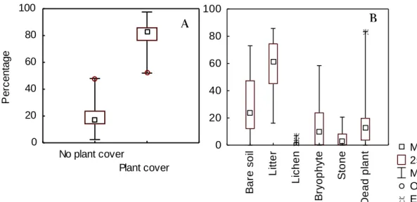
In this work, 15 sites were sampled for plant richness and cover. At each site 246 intercept points were evaluated making a total of 3690 intercept points evaluated along the climatic gradient. The lack of plant was classified as no plant cover. Plant cover was in average 81%. Bugalho et al. (2011) found 83% plant cover in grazed plots under similar climate (mean annual precipitation –MAP- of 587mm) in a study performed in Montado at Alentejo.
Figure 6A shows plant cover variation along all 15 sampled sites.
Figure 6: Median, 25th and 75th percentiles, minimum and maximum, outliers and
extreme values of A: percentage of plant cover and no plant cover; B: percentage of bare soil, litter, lichen and bryophyte within the no-plant cover, in 15 sites sampled along a climatic gradient in Alentejo region.
No plant cover Plant cover 0 20 40 60 80 100 P e rc e n ta g e Median 25%-75% Min-Max Outliers Extremes B a re s o il L it te r L ic h e n B ry o p h y te S to n e D e a d p la n t 0 20 40 60 80 100 B A
22
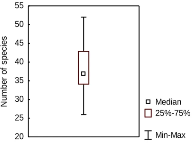
The variable no plant cover was classified for the presence of: bryophytes (15.3%), lichens, litter (56.9%), dead plant, stone/rock, and bare soil (28.4%) (Fig. 6B). The observed low cover of lichens is probably related to the land-use intensity of the Montado ecosystem, namely trampling. Lichens were shown to be very sensitive to disturbance, namely to livestock trampling as shown by Zubiri (2012). A total of 146 plants species were identified and on average there were 36.5 plant species per sampling site, ranging between 26 and 52 (fig.: 7).
Figure 7: Median, 25th and 75th percentiles, minimum and maximum value of number
of species, in all sites sampled (15 sites), along a climatic gradient in Alentejo region.
Castro et al. (2010) found a lower number of plant species (75 species) in plots under extensive grazing and submitted to a climate slightly drier than ours (MAP=438mm and MAT-mean annual temperature=16.8ºC). This could be due to the fact that in the mentioned study only 3 sampling sites were used to measure plant diversity while we measured in 15 different sampling sites. Castro et al. (2010), found a lower median of species per plot (25) ranging from 15 to 38 species based on the observation of 15 plots per site, each with 0.25m2. Castro et al.
(2010) used an area-based method. Nevertheless our driest sites (MAP=521-526mm) showed comparable number of species (26-37) suggesting that climate is an important variable driving biodiversity in this ecosystem.
Median 25%-75% Min-Max 20 25 30 35 40 45 50 55 N u m b e r o f s p e c ie s
23 Under similar climate, Bugalho et al. (2011), found lower plant species (53) than the ones found in this work. The latter author evaluated less plots/sites (5 against 15 sites measured in our study) and had lower total number of intercept points (1440 against 3690) than the ones used in this study. A lower median number of species among the grazed plots (22 species, from 13 to 26) was also found in the study of Bugalho et al. (2011) compared to our results. The authors used the pin-point quadrat method, in which needles are positioned in plots using a frame, with 288 intercept points per plot and a total of 1440 intercept points in grazed plots.
We suspect that distance between intercept points is lower than the used in the present study (0.5m), because frames have 9 needles, positioned 8 times in sub-plots with 2 x 4m. Thus, the lower number of species per plot can probably be due to smaller distance between intercept points, capturing probably lower spatial heterogeneity. One of the main characteristics of drylands is their increasing spatial heterogeneity with increasing aridity. Thus having methods that enable to capture the spatial heterogeneity is of high interest (Kefi et al. 2007).
3.1.2. Diversity of families and of functional groups
Of the 5990 plants collected in 251 hits (4.2%) was not possible to identify plants at the species level. Most of the unidentified individuals were grasses without flowers (88.04% of all unidentified hits), so it was only possible to identify to the family level. The families with higher number of species were Gramineae, Leguminosae and Compositae (Table 3). These three families are also dominant in terms of relative cover in the community (more than 70% except in one site, where it was only 57%).
24
Table 3: Number of species per family found in 15 sites sampled along a climatic gradient in Alentejo region.
Family Nr species Family Nr species
Gramineae 37 Rubiaceae 2 Leguminosae 29 Boraginaceae 1 Compositae 22 Convolvulaceae 1 Caryophyllaceae 12 Cyperaceae 1 Plantaginaceae 6 Euphorbiaceae 1 Cistaceae 5 Gentianaceae 1 Geraneaceae 4 Guttiferae 1 Scrophulariaceae 4 Isoetaceae 1 Brassicaceae 3 Juncaceae 1 Polygonacea 3 Linaceae 1 Labiatae 2 Primulaceae 1 Campanulaceae 2 Umbelliferae 1 Liliaceae 2
Of all species identified, 138 are herbaceous and 8 are shrubs. The number of species (fig.: 8A) and the relative cover (fig.: 8B) of herbaceous plants was much higher than that of shrubs. On average, there was only 1 shrub and 3.6% of the shrub cover per site. The herbaceous layer clearly dominates, with an average of 35.6 species and 96.1% of relative cover per site. This low abundance of shrubs is expected in Montado, since shrubs are intentionally cleared out for the pastures maintenance (Castro and Freitas 2009). The study of Castro (2008), in the same region and ecosystem, with similar climatic features (MAP of 438mm and MAT of 16.8ºC), found that herbaceous species had a relative cover of more than 90%, similar to what we found in our work.