EUROPEAN ORGANIZATION FOR NUCLEAR RESEARCH (CERN)
CERN-EP-2017-330 2018/05/29
CMS-EXO-16-004
Search for decays of stopped exotic long-lived particles
produced in proton-proton collisions at
√
s
=
13 TeV
The CMS Collaboration
∗Abstract
A search is presented for the decays of heavy exotic long-lived particles (LLPs) that are produced in proton-proton collisions at a center-of-mass energy of 13 TeV at the CERN LHC and come to rest in the CMS detector. Their decays would be visible during periods of time well separated from proton-proton collisions. Two decay sce-narios of stopped LLPs are explored: a hadronic decay detected in the calorimeter and a decay into muons detected in the muon system. The calorimeter (muon) search covers a period of sensitivity totaling 721 (744) hours in 38.6 (39.0) fb−1 of data col-lected by the CMS detector in 2015 and 2016. The results are interpreted in several scenarios that predict LLPs. Production cross section limits are set as a function of the mean proper lifetime and the mass of the LLPs, for lifetimes between 100 ns and 10 days. These are the most stringent limits to date on the mass of hadronically decaying stopped LLPs, and this is the first search at the LHC for stopped LLPs that decay to muons.
Published in the Journal of High Energy Physics as doi:10.1007/JHEP05(2018)127.
c
2018 CERN for the benefit of the CMS Collaboration. CC-BY-4.0 license
∗See Appendix A for the list of collaboration members
1
1
Introduction
Heavy long-lived particles (LLPs) on the order of 100 GeV are not present in the standard model (SM). Therefore, any sign of them would be an indication of new physics. Many extensions of the SM predict the existence of LLPs [1–8]. At the CERN LHC, the LLPs will stop inside the detector material if they lose all of their kinetic energy while traversing the detector, which will typically occur for particles with initial velocities less than about 0.5c [9]. This energy loss can occur via nuclear interactions if they are strongly interacting and/or through ionization if they are charged. The observation of a stopped particle decay signature would not only indicate new physics but also help measure the lifetime of LLPs, giving insights into various beyond the standard model (BSM) theories.
If these stopped LLPs have lifetimes longer than tens of nanoseconds, most of their decays would be reconstructed as separate events unrelated to their production [10]. Owing to the dif-ficulty of differentiating between the LLP decay products and SM particles from LHC proton-proton (pp) collisions, these subsequent decays are most easily identified when there are no proton bunches in the detector. The detector is quiet during these out-of-collision time periods with the exception of rare noncollision backgrounds, such as cosmic rays, beam halo particles, and detector noise. If LLPs come to a stop in the detector, they are most likely to do so in the densest detector materials, which in the CMS detector are the electromagnetic calorime-ter (ECAL), the hadron calorimecalorime-ter (HCAL), and the steel yoke in the muon system. If the stopped LLPs decay in the calorimeters, relatively large energy deposits occurring in the inter-vals between collisions could be observed. Furthermore, if the stopped LLPs decay into muons, displaced muon tracks out of time with the collisions could be detected.
In this paper we present two searches for stopped LLPs that decay out of time with respect to the presence of proton bunches in the detector. One search targets hadronic decays detected in the calorimeters, and the other looks for decays to muon pairs in the muon system. These two search channels are analyzed independently using data collected by the CMS experiment
in 2015 and 2016 with separate dedicated triggers. The calorimeter (muon) search uses√s =
13 TeV data corresponding to an integrated luminosity of 38.6 (39.0) fb−1 collected with LHC
pp collisions separated by 25 ns during a search interval totaling 721 (744) hours. The size of the search sample is further reduced by applying a series of offline selection criteria to decrease the number of events that most likely come from the primary sources of background.
The calorimeter search presented here improves upon previous searches performed by the CMS
Collaboration, the most recent of which used √s = 8 TeV pp collision data corresponding to
an integrated luminosity of 18.6 fb−1 collected in 2012 [11]. This search excluded long-lived
gluinos (eg) with masses below 880 GeV and long-lived top squarks (et) with masses below
470 GeV, for lifetimes between 10 µs and 1000 s. The results of earlier, similar searches have been reported by the D0 Collaboration at the Tevatron [12] and by the CMS [13, 14] and AT-LAS Collaborations [15, 16]. The displaced muon search is newly added to investigate different models with leptonic decays of stopped LLPs, such as those of gluinos [9] and multiply charged massive particles (MCHAMPs) [17–20]. Searches for decays of stopped LLPs are complemen-tary to searches for heavy stable charged particles (HSCPs) that pass through the detector and can be identified by their energy loss and time-of-flight (TOF) information [21–34]. The searches presented here would allow the study of the decay of such heavy particles, whereas dedicated HSCP searches typically look for the particle itself, before it decays. However, both the searches for decays of stopped LLPs and for HSCPs are sensitive to a similar range of lifetimes.
2
The CMS detector
The central feature of the CMS apparatus is a superconducting solenoid of 6 m internal diame-ter, providing a magnetic field of 3.8 T. Within the solenoid volume are a silicon pixel and strip tracker, a lead tungstate crystal ECAL, and a brass and scintillator HCAL, each composed of a barrel and two endcap sections. Forward calorimeters extend the pseudorapidity η coverage provided by the barrel and endcap detectors. In the region |η| < 1.74, the HCAL cells have widths of 0.087 in η and 0.087 radians in azimuth (φ). In the η-φ plane, and for |η| < 1.48,
the HCAL cells map on to 5×5 arrays of ECAL crystals to form calorimeter towers projecting
radially outwards from close to the nominal pp collision interaction point (IP). For|η| > 1.74,
the coverage of the towers increases progressively to a maximum of 0.174 in∆η and ∆φ. Within
each tower, the energy deposits in ECAL and HCAL cells are summed to define the calorimeter tower energies, which are subsequently used to provide the energies and directions of hadronic jets. In the HCAL barrel (HB) and endcap, scintillation light is detected by hybrid photodiodes (HPDs), and each HPD collects signals from 18 different HCAL channels. Signals from four HPDs are then digitized by analog-to-digital converters within a single readout box (RBX). Muons are measured in gas-ionization chambers embedded in the steel flux-return yoke
out-side the solenoid. Muons are measured in the range |η| < 2.4, with detection planes made
using three technologies: drift tubes (DTs) in the barrel, cathode strip chambers (CSCs) in the endcaps, and resistive plate chambers (RPCs) in both the barrel and the endcaps. All these tech-nologies provide both position and timing information. Hits within each DT or CSC chamber are matched to form a reconstructed DT or CSC segment.
The first level (L1) of the CMS trigger system, composed of custom hardware processors, uses information from the calorimeters and muon detectors to select the most interesting events in a fixed time interval of less than 4 µs. The high-level trigger processor farm further decreases the event rate from around 100 kHz to less than 1 kHz, before data storage.
A more detailed description of the CMS detector, together with a definition of the coordinate system used and the relevant kinematic variables, can be found in Ref. [35].
3
Data and Monte Carlo simulation
3.1 Data samples
The LHC accelerates two proton beams in opposite directions such that the protons collide at several points along the LHC ring, including one at the CMS detector. Each LHC beam consists of a number of proton bunches arranged into an irregular pattern of “trains” [36]. Within a train, the proton bunches are nominally spaced 25 ns apart, with a larger spacing between trains to account for the needs of the injection process. In an LHC orbit there are 3564 bunch slots (BXs), which are 25 ns long. Each BX could be filled with proton bunches, which usually occupy the first 2.5 ns of the BX, or could be empty. The trains may be spaced such that there could be multiple empty BXs between filled BXs. To search for LLP decays during these empty BXs, dedicated triggers select events at least two BXs away from any proton bunches. Thus these triggers are live only during these specific time windows. This distance of two BXs is chosen so that we maximize the search time window while suppressing most of the events from secondary pp interactions and from “beam halo”, which are mostly muons traveling outside the LHC beam that are produced by LHC beam–collimator scattering.
The search is performed with√s = 13 TeV pp collision run data collected by the CMS
3.2 Benchmark models 3
November 2015, corresponds to an integrated luminosity of 2.7 (2.8) fb−1 and spans a trigger
livetime, which is the amount of time the triggers are live in between collisions, of 135 (155) hours. The 2016 calorimeter (muon) search sample was taken between May and October 2016,
during which a data sample corresponding to an integrated luminosity of 35.9 (36.2) fb−1 was
recorded, spanning a trigger livetime of 586 (589) hours. We do not consider the possibility of LLPs that were produced in 2015 but decayed in 2016. In both the 2015 and 2016 searches, we use cosmic run data collected by dedicated triggers as a control sample. These dedicated cos-mic run data were recorded during LHC machine technical stops, several days after collision runs. A negligible amount of long-lived signal produced during collisions could have decayed during these cosmic runs for the lifetimes considered in this analysis. The instrumental noise background estimate is extrapolated from the instrumental noise measured in these control samples. Most of the other sources of background are estimated from sideband regions of the main data sample, except for the cosmic ray muon background in the calorimeter search, which is estimated from MC simulation.
3.2 Benchmark models
Several simplified models are considered in this search, and samples are generated for each using Monte Carlo (MC) simulation.
In the calorimeter search, we interpret the results in the context of two-body (eg → gχe
0) and
three-body (eg → qqχe
0) decays of a gluino into the lightest supersymmetric (SUSY) particle
(LSP), the neutralino (χe
0). Long-lived gluinos are predicted by “split SUSY” [37, 38], in which
gauginos have relatively small masses with respect to sfermions, which could be massive, since SUSY is broken at a scale much higher than the weak scale. This large mass splitting causes the long lifetime of the gluinos, since gluinos can only decay via a virtual squark. We also consider the decay of a long-lived top squark (et → tχe
0) that can be the next-to-LSP particle (NLSP) in
various dark matter scenarios [39–41]. Here the LSP should be loosely interpreted as any new, neutral, non-interacting fermion, and not necessarily as a SUSY neutralino.
In the muon search, we consider a different model for a three-body decay of the gluino (eg →
qqχe
0 2,χe
0
2 → µ+µ−χe
0), which is complementary to the calorimeter search. In this model, the
mass of the LSP neutralino (χe
0) is chosen to be 0.25 times the gluino mass, and the mass of the
NLSP neutralino (χe
0
2) is chosen to be 2.5 times the LSP neutralino mass. A second simplified
model used in the muon search predicts exotic particles called MCHAMPs, whose charges are multiples of the elementary charge e and which are predicted by several BSM theories [20]. We
assume an MCHAMP with charge|Q| = 2e decays into two same-sign muons (MCHAMP→
µ±µ±).
3.3 Signal generation
The signal generation process is divided into three major stages. In Stage 1, the LLPs for each
signal process are generated from pp collisions withPYTHIA[42, 43] and propagated through
the detector with GEANT4 v9.2 [44, 45]. For the MCHAMP signal,PYTHIA v6.4 is used, while
for the gluino and top squark signals, PYTHIA v8.205 is used. If the LLPs are strongly
inter-acting, as in the case of the gluinos and top squarks, they hadronize into R-hadrons [46–48] upon production, whose interaction with the CMS detector in the simulation is described by the cloud model [49, 50]. In this model, R-hadrons are treated as SUSY particles surrounded by a cloud of loosely bound quarks and gluons. The fraction of produced R-hadrons that contain a gluino and a valence gluon is set to 10%, a convention used in previous analyses [11, 21]. How-ever, because the R-hadrons interact an average of ten times in the calorimeter, their flavor is effectively randomized. Some fraction of these R-hadrons are sufficiently slow moving to come
to a stop in the detector material. Because they are doubly charged, MCHAMPs ionize heavily and thus a significant number also stop in the detector.
In Stage 2, the parent LLP or R-hadron is constrained to decay at the stopping position defined
in Stage 1. The LLP decay is simulated by a second GEANT4 step, and the decay products are
propagated through the detector.
Finally, in Stage 3, a pseudo-experiment MC simulation is conducted to estimate the probability for stopped particle decays to occur in the time window between collisions when data is being collected. The Stage 3 MC simulation determines an effective integrated luminosity by using the good data-taking periods and the LHC filling scheme to calculate the fraction of stopped particle decays that occur when the trigger is live. For a given particle lifetime, the effective integrated luminosity is defined as the total integrated luminosity multiplied by the probability that the particle decays at a time when the trigger is live in between collisions. In other words, Stages 1 and 2 determine how the signal will look in the detector, and Stage 3 determines when it will occur. More details on the signal generation process are given in Refs. [11, 13, 14].
4
Event selection
The calorimeter search and the muon search employ different search strategies and thus differ-ent selection criteria, which are described in turn below.
4.1 Calorimeter search
In the calorimeter search, we look for hadronic decays of LLPs in the calorimeter that produce energy deposits that could be reconstructed as at least one high-energy jet. We trigger on cal-orimeter jets with energy greater than 50 GeV and|η| <3 that are at least two BXs away from pp collisions.
The major background sources are cosmic rays, beam halo, and HCAL noise. Cosmic ray and beam halo muons can emit a shower of photons via bremsstrahlung, which could be recon-structed as a jet and mistaken for signal. HCAL noise [51] can give rise to spurious signals, which in the barrel could appear in one or several HPDs within a single RBX, and thus be in-correctly reconstructed as a jet. We observe that the rate of each of these background sources drops exponentially as a function of the jet energy. We thus require the events to have a leading (highest energy) calorimeter-based jet with energy greater than 70 GeV. The calorimeter-based jets are reconstructed using an anti-kT clustering algorithm [52, 53] with a distance parameter
of 0.4. To increase the sensitivity of the search, we require that the leading jet in each event is located within|η| <1.0, where R-hadrons are more likely to stop and where there is relatively less background from beam halo.
Secondary background sources include out-of-time collisions from remnant protons between bunches, and beam-gas interactions in the detector. The rate of these secondary background events becomes negligible after we require that there are no reconstructed collision vertices in the events.
Cosmic ray muon events usually feature a large number of reconstructed DT segments and RPC hits, whereas signal events in the calorimeter search would not. We exploit this difference to distinguish signal events from cosmic ray muons. While it is possible for the hadronic shower of an R-hadron decay to pass through the first layers of the iron yoke and induce reconstructed DT segments, these DT segments are located only in the inner layers of the muon chambers (r < 560 cm, where r is the transverse distance to the IP) and cluster near the leading jet. On
4.2 Muon search 5
the other hand, cosmic ray muons are equally likely to leave DT segments in all layers in both the upper and lower hemispheres of the muon system, and the angle between the jet and DT segments in φ is more evenly distributed. As a result, we are able to substantially reduce the cosmic ray muon background contamination in the signal region by rejecting events that have at least two DT segments in the outermost barrel layer of the muon system, events that have any DT segments in the second outermost barrel layer, events that have two DT segments with a large separation in φ (|∆φ| > π/2), events that have DT segments in the three innermost layers that are separated in φ from the leading jet by at least 1.0 radian, and events that have
close-by RPC hits in different layers (∆R=
√
(∆φ)2+ (∆η)2 < 0.2 and∆r> 0.5 m). We make looser DT segment requirements in the outermost than in the second outermost layer because signals are very likely to coincide with standalone DT segments that are not from cosmic ray muons but particles from the pp collision. Most of these standalone DT segments from the pp collision are located in the outermost muon barrel layer. With these selection criteria, we are able to avoid incorrectly rejecting signal events, thus increasing the signal efficiency, while still rejecting most of the cosmic ray muon events.
Beam halo muons travel closely along the beam pipe, typically traversing both sides of the muon endcap systems and resulting in a few reconstructed CSC segments. Therefore, we veto events with any CSC segments having at least five reconstructed hits. As will be discussed in Section 5, since signal events may include some CSC segments, requiring a minimum number of CSC hits in the veto avoids a loss of signal efficiency.
Random electronic noise in the HCAL gives rise to events in which the time response of the HCAL readout is very different from the well-defined response from particles showering in the calorimeter. This HCAL noise creates spurious clustered energy deposits that can be recon-structed as a jet, which would contaminate the signal region and therefore should be removed. Analog signal pulses produced by the HCAL electronics are read out over ten BXs centered around the pulse maximum. The pulse shape from showering particles consists of a peak at the collision BX and an exponential decay over the subsequent BXs. Particle showers create clustered energy deposits spread over several neighboring calorimeter towers in z and φ, while noise produces deposits in just one or two towers, or several towers in a single HPD or RBX. In addition to the standard HCAL noise filter [51], we use a series of offline selection criteria that exploit these timing and topological characteristics to remove the HCAL noise events. These criteria are described in detail in Ref. [14].
4.2 Muon search
In the muon search, we look for LLPs where the decay products include two muons. We expect the signal to look like a pair of muons originating anywhere in the detector material, but dis-placed from the IP. The muons would be back-to-back in the two-body MCHAMP decay, but not for the three-body gluino decay.
The primary background sources in the muon search include cosmic ray muons, beam halo, and muon detector noise. The latter two background sources are negligible after we apply the full selection.
The trigger used in the muon search selects events at least two BXs away from the pp collision time with at least one muon reconstructed in the muon system, whose transverse momentum pT is at least 40 GeV. As in the calorimeter search, we select events offline that have no
recon-structed collision vertices.
tracks [54]. However, the standard standalone track reconstruction assumes that muons orig-inate from the IP, which is inappropriate for displaced muon searches. As a result, a new muon reconstruction algorithm was developed for this analysis, which produces displaced standalone (DSA) muon tracks [55]. The DSA tracks are reconstructed using only hits in the muon detector, and they have no constraints to the IP. Thus, DSA tracks are truly using only the muon system.
We require events to have exactly one good DSA track in the upper hemisphere of the detector
and exactly one good DSA track in the lower hemisphere. Both DSA tracks must have pT >
50 GeV, at least three DT chambers with valid hits, and at least three valid RPC hits. To reduce the background from beam halo, the DSA tracks must also have zero valid CSC hits.
Timing information in the DTs and RPCs, indicating whether the muon is incoming toward the detector center or outgoing away from the detector center, is used to distinguish muons from a signal event from the cosmic ray muon background. Cosmic ray muons are predom-inantly incoming when traversing the upper hemisphere and outgoing when traversing the lower hemisphere, as they come in from above the detector and continue to move downwards. Muons from a signal event, on the other hand, would be outgoing in both hemispheres. We place selection criteria on both the upper and lower hemisphere DSA tracks in order to obtain a good time measurement. We require at least eight independent time measurements for the TOF computation. We require that the uncertainty in the time measured at the IP for DSA tracks, assuming the muon is outgoing, is less than 5.0 ns.
Next, we ask for the time measurement to be signal-like. We require that the direction of the lower hemisphere DSA track, as determined by a least-squares fit to the timing in each DT layer where the fit is not constrained to the IP, is consistent with being in the downward direction.
We define tDT as the time at the point of closest approach to the IP as measured by the DTs,
assuming the muon is outgoing. Since cosmic ray muons are incoming in the upper hemisphere
and outgoing in the lower hemisphere, the tDTof the upper hemisphere track is expected to be
40 to 50 ns earlier than that of the lower hemisphere track. As for the signal, since both muons are outgoing, they are reconstructed to have similar times as measured at the IP. Thus, we require that∆tDT, which is defined as∆tDT= tDT(upper) −tDT(lower), is greater than−20 ns,
which greatly reduces the cosmic ray muon background.
In addition to these DT timing variables, we use a timing measurement from the RPCs that assigns a BX to each hit. For each of the six layers of the RPCs, the hit is given a BX assignment. A typical prompt muon created at the IP has a BX assignment of 0 for each of its RPC hits. The BX assignments of cosmic ray muons are especially useful in the lower hemisphere of the detector, as the incoming cosmic ray muons will typically trigger the event and thus be assigned BX values of 0 in each RPC layer, but the outgoing cosmic ray muons are often assigned positive BX values. For example, a lower hemisphere cosmic ray muon typically has a BX assignment of 2 for each of its good RPC hits. For the signal, each RPC BX assignment for each muon is typically 0.
Given the BX assignments in each RPC layer for a muon, we can compute the average RPC
hit BX assignment multiplied by 25 ns as the RPC time for a track (tRPC) and use this as a
discriminating variable. A typical muon from the benchmark decays has a tRPCof 0 ns for both
upper and lower hemisphere DSA muon tracks. On the other hand, the tRPCof a cosmic ray
muon is typically 25 or 50 ns in the lower hemisphere and 0 ns in the upper hemisphere. We define∆tRPC = tRPC(upper) −tRPC(lower), and we require ∆tRPC > −7.5 ns to further select
7
Figure 1 shows∆tDT (left) and ∆tRPC (right) for data and MC simulation. The events shown
here contain good-quality DSA muon tracks, but they are dominated by the cosmic muon back-ground; they are selected with a subset of the criteria described above. This selection is defined by the same trigger and reconstructed vertices requirements as above. Additionally, exactly one DSA track in the upper hemisphere and exactly one DSA track in the lower hemisphere
are required. Looser requirements than in the full selection are placed on the DSA track pT
(>10 GeV), the number of DT chambers with valid hits (greater than one), and the number of valid RPC hits (greater than one). We require the same number of DT hits with good timing measurements per DSA track and number of valid CSC hits as above for this selection. None of the remaining criteria from the main selection criteria described above are used to select the events in Fig. 1. As can be seen in Fig. 1, the number of cosmic ray muon background events is greatly reduced when the full selection is applied, as we require∆tDT > −20 ns and
∆tRPC > −7.5 ns. Since ∆tDT and∆tRPC correspond to independent measurements of
essen-tially the same quantity, a mismeasured cosmic ray muon is much less likely to pass both selec-tions than just one; adding the second requirement improves the rejection of simulated cosmic ray muons by a factor of approximately 350.
[ns] DT t ∆ 100 − −50 0 50 100 Fraction of Entries / 5.0 ns 4 − 10 2 − 10 1 2 10 4 10 Data
Cosmic ray muon simulation
0 χ∼ -µ + µ → 2 0 χ∼ , 2 0 χ∼ q q → g ~ = 250 GeV) 0 χ∼ = 625 GeV, m 2 0 χ∼ = 1000 GeV, m g ~ (m = 600 GeV) MCHAMP (|Q| = 2e, m ± µ ± µ → MCHAMP 0 χ∼ -µ + µ → 2 0 χ∼ , 2 0 χ∼ q q → g ~ = 250 GeV) 0 χ∼ = 625 GeV, m 2 0 χ∼ = 1000 GeV, m g ~ (m = 600 GeV) MCHAMP (|Q| = 2e, m ± µ ± µ → MCHAMP CMS (13 TeV) -1 2016: 36.2 fb [ns] RPC t ∆ 100 − −50 0 50 100 Fraction of Entries / 5.0 ns 4 − 10 2 − 10 1 2 10 4 10 Data
Cosmic ray muon simulation
0 χ∼ -µ + µ → 2 0 χ∼ , 2 0 χ∼ q q → g ~ = 250 GeV) 0 χ∼ = 625 GeV, m 2 0 χ∼ = 1000 GeV, m g ~ (m = 600 GeV) MCHAMP (|Q| = 2e, m ± µ ± µ → MCHAMP 0 χ∼ -µ + µ → 2 0 χ∼ , 2 0 χ∼ q q → g ~ = 250 GeV) 0 χ∼ = 625 GeV, m 2 0 χ∼ = 1000 GeV, m g ~ (m = 600 GeV) MCHAMP (|Q| = 2e, m ± µ ± µ → MCHAMP CMS (13 TeV) -1 2016: 36.2 fb
Figure 1: The∆tDT (left) and∆tRPC (right) distributions for 2016 data, MC simulated cosmic
ray muon, 1000 GeV gluino signal, and 600 GeV MCHAMP signal events, for the muon search. The events plotted pass a subset of the full analysis selection that is designed to select good-quality DSA muon tracks but does not reject the cosmic ray muon background. The number of cosmic ray muon background events is greatly reduced when the full selection is applied, as we require ∆tDT > −20 ns and ∆tRPC > −7.5 ns. The gray bands indicate the statistical
uncertainty in the simulation. The histograms are normalized to unit area.
5
Signal efficiency
In this section, we describe the calculation of the signal efficiency εsignal, which is the product of
several efficiencies. In the calorimeter search, the stopping efficiency εstoppingis the probability
that the R-hadron stops in the HB or ECAL barrel (EB), while in the muon search, εstoppingis the
probability of each LLP to stop in any region of the detector. The Stage 1 simulation determines εstopping. The reconstruction efficiency εrecois the efficiency of an event to pass all of the selection
criteria, including the trigger, and it is computed independently of εstopping. In addition, εrecois
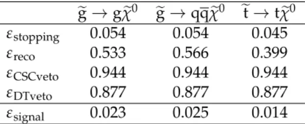
Table 1: Summary of the values of εstopping, εCSCveto, εDTveto, and the plateau value of εrecofor
different signals, for the calorimeter search. The efficiency εstoppingis constant for the range of
signal masses considered. The efficiency εrecois given on the Egor Etplateau for each signal.
e g→gχe 0 e g→qqχe 0 et→tχe 0 εstopping 0.054 0.054 0.045 εreco 0.533 0.566 0.399 εCSCveto 0.944 0.944 0.944 εDTveto 0.877 0.877 0.877 εsignal 0.023 0.025 0.014
and assuming a branching fraction (B) of 100% to the decays in the signal models described
above. The Stage 2 simulation determines εreco. The efficiency εsignalis defined as the product
of εstopping and εreco for the muon search. For the calorimeter search, εsignal is the product of
εstopping, εreco, and two additional factors, εCSCveto and εDTveto, which are defined in the next
subsection.
5.1 Calorimeter search
For the calorimeter search, εstopping is constant at about 0.054 for gluinos and 0.045 for top
squarks, for the range of masses considered. The εstopping value is larger for gluinos than for
top squarks of the same mass because gluinos are more likely to produce doubly charged R-hadrons.
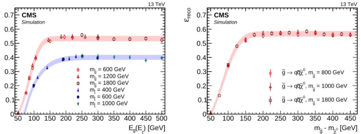
The value of εreco depends primarily on the energy of the visible daughter particle(s) of the
R-hadron decay, denoted by Eg(Et) if the daughter is a gluon (top quark). When Eg>130 GeV
(Et > 170 GeV), εrecobecomes approximately constant, as shown in Fig. 2. For the three-body
gluino decay, εrecodepends approximately on the mass difference betweeneg andχe
0, becoming
constant when meg−mχe0 &160 GeV.
Some physical effects that are not modeled in simulation can cause reconstructed CSC or DT segments that are out of time with respect to a collision. For example, thermal neutrons can take up to a tenth of a second after being produced in pp collisions before they arrive at the muon detectors and induce a signal in the CSCs or DTs. Since these segments can occur when the trigger is live, it is possible that some of the events in the search sample could contain such segments. These events would be rejected by the selection criteria, thus decreasing the probability for a signal to be observed. The terms εCSCvetoand εDTvetomeasure this decrease in
efficiency due to these sources.
We define εCSCveto (εDTveto) as the conditional probability that a signal passes the beam halo
(cosmic ray muon) rejection criteria assuming the potential occurrence of coincident CSC (DT) segments, given that the signal itself passes the full selection criteria. HCAL noise events that are collected by the trigger are used to estimate these two efficiencies from data, since this noise is independent of any muon detector activities and should pass both beam halo rejection and cosmic ray muon rejection criteria. These events are selected by inverting some of the noise rejection criteria. Then εCSCveto (εDTveto) is simply the percentage of noise events that survive
the beam halo (cosmic ray muon) vetoes among all selected noise events.
5.2 Muon search 9 ) [GeV] t (E g E 50 100 150 200 250 300 350 400 450 500 reco ε 0 0.1 0.2 0.3 0.4 0.5 0.6 0.7 = 600 GeV g ~ m = 1200 GeV g ~ m = 1800 GeV g ~ m = 400 GeV t ~ m = 600 GeV t ~ m = 1000 GeV t ~ m 13 TeV CMS Simulation [GeV] 0 χ∼ - m g ~ m 50 100 150 200 250 300 350 400 450 reco ε 0 0.1 0.2 0.3 0.4 0.5 0.6 0.7 = 800 GeV g ~ , m 0 χ∼ q q → g ~ = 1000 GeV g ~ , m 0 χ∼ q q → g ~ = 1800 GeV g ~ , m 0 χ∼ q q → g ~ 13 TeV CMS Simulation
Figure 2: The εreco values as a function of Eg or Et(left), and meg−mχe0 (right), foreg andet
R-hadrons that stop in the EB or HB, in the MC simulation, for the calorimeter search. The εreco
values are plotted for the two-body gluino and top squark decays (left) and for the three-body gluino decay (right). The shaded bands correspond to the systematic uncertainties, which are described in Section 7.
5.2 Muon search
Tables 2 and 3 show εstoppingand εreco for each assumed signal mass in the muon search. The
εsignalvalue is the product of these two efficiencies. The εstoppingvalue is larger for MCHAMPs
than for gluinos because the MCHAMPs considered have|Q| =2e and the gluinos sometimes
produce singly charged R-hadrons. We lose signal efficiency because the L1 muon trigger is designed to identify muons coming from the IP, although the muons from the signal can be very displaced. A further loss in signal efficiency is due to the very strict requirements on the quality of the DSA muon track. Similarly, the requirement to have exactly one DSA track traversing the upper hemisphere and exactly one DSA track traversing the lower hemisphere further reduces the geometrical acceptance, particularly for the gluino decay, which does not produce back-to-back muons, unlike the MCHAMP decay. The numbers in Tables 2 and 3 represent the maximum number of signal events that can be measured before applying the different search windows depending on the lifetime of the stopped particle.
Table 2: Gluino εstopping and εreco, as well as the number of expected gluino events with
life-times between 10 µs and 1000 s, assuming B(eg → qqχe
0 2)B(χe
0
2 → µ+µ−χe
0) = 100%, for each
mass point considered for the 2016 muon search. The efficiencies are constant for this range of lifetimes.
meg[GeV] εstopping εreco Expected events
400 0.19 0.0015 400 600 0.17 0.0024 50 800 0.17 0.0037 10 1000 0.17 0.0029 2 1200 0.18 0.0025 0.5 1400 0.20 0.0031 0.2 1600 0.21 0.0029 0.1
6
Background estimation
Since the background sources in both the calorimeter and the muon searches are not well mod-eled in simulation, we use control samples in data to estimate their contributions after the full
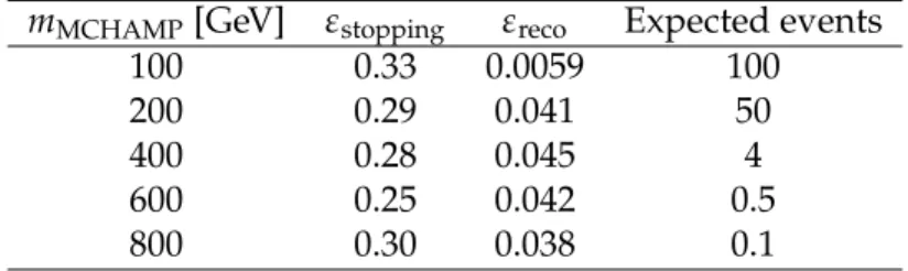
Table 3: MCHAMP εstopping and εreco, as well as the number of expected MCHAMP events
with lifetimes between 10 µs and 1000 s, assumingB(MCHAMP → µ±µ±) = 100%, for each
mass point considered for the 2016 muon search. The efficiencies are constant for this range of lifetimes.
mMCHAMP[GeV] εstopping εreco Expected events
100 0.33 0.0059 100
200 0.29 0.041 50
400 0.28 0.045 4
600 0.25 0.042 0.5
800 0.30 0.038 0.1
event selection is applied.
6.1 Calorimeter search
After applying the selection criteria in the calorimeter search, some background sources from cosmic ray muons, beam halo, and calorimeter noise remain in the data. We quantify the prob-ability of background events escaping the background vetoes and thus being observed by this search. These inefficiencies are calculated as follows.
We generate a sample of cosmic ray muon events to estimate the rate of such events escaping
the cosmic ray muon rejection criteria. The events are generated using CMSCGEN[56], a
gen-erator based on the air shower program CORSIKA [57] and validated in a CMS analysis [58].
We require that the events pass the preselection criteria, namely that they are required to have substantial energy deposits in the calorimeter and no CSC segments in the muon endcap sys-tem. The cosmic ray muon veto inefficiency is defined as the fraction of preselected simulated cosmic ray muon events that are not rejected by the cosmic ray muon rejection criteria. It is
found to be 1×10⁻³. To account for the small difference in occupancy between the cosmic
ray muon events in data and MC simulation, we first bin the simulated events in the number of DT and outer barrel RPC hits and calculate the inefficiency bin by bin. Then, we apply the halo veto and the noise veto to a sample of events in data, and bin these data events in the same way as the simulated events. For each bin, we multiply the inefficiency by the number of events in data, giving the binned cosmic ray muon prediction. The nominal cosmic ray muon background prediction is then the sum of the events in each bin.
The uncertainty in the cosmic ray muon background is due to the uncertainty in the estimate of muons that escape detection by passing through uninstrumented regions of the CMS detec-tor, which is necessarily estimated from simulation. Since data in the uninstrumented regions are ipso facto not available to compare to simulation, we define equivalent fiducial volumes of instrumented regions of the muon system. Using these as a proxy for the uninstrumented re-gions, we assess the reliability of the simulation by comparing data and simulation. We find the average discrepancy between cosmic ray muon data and simulation in the number of detected muons traveling through various fiducial regions in the detector to be about 32%, and we as-sign this to be the systematic uncertainty in the cosmic ray muon background estimate. Thus,
we estimate the cosmic ray muon background to be 2.6±0.9 (8.8±3.1) events in 2015 (2016)
data.
Because there was a high rate of beam halo production in 2015 and 2016 data, and because it is possible for halo muons to escape the acceptance of the endcap muon system, the halo background is nonnegligible. We estimate the halo veto inefficiency using a tag-and-probe method [59] that analyzes a high-purity sample of halo events by selecting events having one
6.2 Muon search 11
calorimeter jet with |η| < 1.0 and CSC segments in at least two endcap layers of the muon
system. Since the rates of beam halo in each beam are not the same, the events are first classi-fied according to whether they originated in the clockwise (−z direction) or the
counterclock-wise (+z direction) beam. Then for each class, depending on whether these events have CSC
segments in only one endcap or both endcaps of the muon system, they are categorized into events that have only the incoming portion of a halo muon track, events that have only the outgoing portion, and events that have both portions. The number of events that escape detec-tion is NIncomingOnlyNOutgoingOnly/NBoth. We define NIncomingOnly (NOutgoingOnly) as the number
of events that have only an incoming (outgoing) portion of a halo muon track. The number
of events that have both an incoming and an outgoing halo muon track is NBoth. After
bin-ning halo events in their x and y coordinates and performing the classification and calculation discussed above, we estimate the halo veto inefficiency to be 1×10⁻⁴. We then multiply this
inefficiency by the number of halo events vetoed in the search region.
To account for the possibility that the x-y binning does not reproduce the actual shape of the inactive or uninstrumented regions of the detector, thus biasing the estimate, we repeat the calculation above, but binning events in φ and r instead. The systematic uncertainty is then defined as the difference between the results from the two binning schemes. We find a halo background estimate of 1.1±0.1 (2.6±0.2) events in 2015 (2016) data.
Finally, the background estimation of instrumental noise is performed using control data in dedicated cosmic runs with no beams in the LHC, which include only cosmic ray muon and noise events. We select cosmic runs taken several days after pp collision runs so that there would be little chance for the signal to appear. After applying all selection criteria on the con-trol data, we observe 2 events in each of the 2015 and 2016 concon-trol data. We then subtract the expected cosmic ray muon background from the total event yield, obtaining a noise back-ground estimate of 0.3+−2.40.3 (0.0+−2.20.0) events in 2015 (2016) control data. Based on the number of noise events in the control sample, we expect the noise veto inefficiency to be≤ 1×10⁻⁴. These noise estimates are then scaled to the search data, assuming that the noise veto ineffi-ciency remains the same. The resulting noise background estimate is 0.4+−2.90.4(0.0+−9.80.0) events in 2015 (2016). The uncertainty in the 2016 prediction is large because the trigger livetime of the cosmic runs in 2016 was about 60% shorter than that of the collision runs, and also because the 2016 trigger livetime in collision runs is larger than the 2015 trigger livetime. Therefore, the uncertainty is scaled by a larger factor.
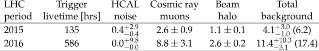
The total background estimate for the calorimeter search is 4.1+−3.01.0 (11.4+−10.33.1 ) events in 2015 (2016), as summarized in Table 4.
Table 4: The background prediction for the calorimeter search. The total background median value is listed in parentheses; this value corresponds directly to the median expected limits shown below.
LHC Trigger HCAL Cosmic ray Beam Total
period livetime [hrs] noise muons halo background
2015 135 0.4+−2.90.4 2.6±0.9 1.1±0.1 4.1+−3.01.0(6.2)
2016 586 0.0+−9.80.0 8.8±3.1 2.6±0.2 11.4+−10.33.1 (17.4)
6.2 Muon search
In the muon search, a small number of cosmic ray muon background events remains after ap-plying the full event selection to the data. The cosmic ray muon background is estimated by extrapolating the data from a background-dominated region into the signal region. We
ap-ply the full event selection to the data except the∆tDTcriterion and invert the∆tRPCcriterion.
We then fit the ∆tDT distribution with the sum of two Gaussian distributions and a Crystal
Ball function [60], since ∆tDT is relatively Gaussian with a long asymmetrical tail. Next, we
compute the integral of the fit function, for∆tDT > −20 ns. Then, we compute the same
in-tegral after having tightened the selection criteria on∆tRPCto −50 < ∆tRPC < −7.5 ns, then
−45 < ∆tRPC < −7.5 ns, etc. in steps of 5 ns up to−10 < ∆tRPC < −7.5 ns. Finally, we plot each integral as a function of the lower selection on∆tRPC, and fit this with an error function
to extrapolate to the∆tRPC > −7.5 ns region (see Fig. 3). We use an error function fit in order
to make a conservative background estimate. Given this extrapolation, we predict 0.04 back-ground events in 2015 data, with a negligible statistical uncertainty, and 0.50±0.02 background events in 2016 data, where the uncertainty given is statistical only. The statistical uncertainty in the background prediction derives from the uncertainty in the error function fit parameters. We checked the background prediction method by repeating the procedure with
nonoverlap-ping∆tRPCregions and found that the numbers of background events predicted are consistent
with the nominal values.
threshold [ns] RPC t ∆ Lower 100 − −80 −60 −40 −20 0 20 ns − > DT t ∆
Fit integral for
1 − 10 1 10 2 10 3 10 2015 data 2016 data (13 TeV) -1 2015 + 2016: 39.0 fb CMS
Figure 3: The background extrapolation for the muon search. The integral of the fit function to ∆tDTwith the sum of two Gaussian distributions and a Crystal Ball function, for∆tDT> −20 ns,
is plotted as a function of the lower ∆tRPC selection, for 2015 (red squares) and 2016 (black
circles) data. The points are fitted with an error function and used to extrapolate to the signal region, which is defined as∆tRPC> −7.5 ns.
The systematic uncertainty in the background prediction is evaluated by repeating the steps
above, except changing the fit of the∆tDT distribution to the sum of two Gaussian
distribu-tions and a Landau function [61]. Using the error function fits to extrapolate to∆tRPC> −7.5 ns
gives a prediction of 0.07±0.06 (0.10±0.01) background events in 2015 (2016), where the uncer-tainty given is statistical only. Thus, the background prediction is: 0.04±0.03 (syst) background events in 2015 data, with a negligible statistical uncertainty, and 0.50±0.02 (stat)±0.40 (syst) background events in 2016 data.
Despite the fact that we require exactly one upper hemisphere DSA track and exactly one lower hemisphere DSA track, there could still be some background from two coincident cosmic ray muons. This background from two coincident cosmic ray muons could occur if the upper hemi-sphere DSA track of one cosmic ray muon is reconstructed and if the lower hemihemi-sphere DSA
13
track of the other is also reconstructed. We estimate this contribution from data by finding the rate of events with exactly one reconstructed DSA track in one hemisphere satisfying all of the selection criteria except for the∆tDTand∆tRPCcriteria, and no tracks in the other hemisphere.
Then, making simple assumptions about when the two coincident cosmic ray muons could occur and about the DSA track reconstruction efficiency as a function of BX, we calculate the number of accidentally coincident cosmic ray muons and find it to be negligible.
7
Systematic uncertainties in the signal efficiency
While the GEANT4 simulation used to derive the stopping probability accurately models both
the electromagnetic and nuclear interaction energy loss mechanisms, the relative contributions of these energy loss mechanisms to the stopping probability depend significantly on unknown R-hadron spectroscopy. We do not consider this dependence to be a source of uncertainty for either the calorimeter or the muon search, however, since for any given model the resultant uncertainty in the stopping probability is small. Nevertheless, there are several sources of uncertainty in the signal efficiency measurement.
7.1 Calorimeter search
In the calorimeter search, the systematic uncertainty due to the trigger efficiency is negligible since the offline jet energy criterion ensures the data analyzed are well above the turn-on region, so εreco is constant. We consider possible systematic uncertainties in εCSCveto and εDTveto by
varying the criteria used to select HCAL noise events that were described in Section 5.1. We compare the efficiency of data events to pass these new HCAL noise criteria with that of the nominal HCAL noise selection criteria, and we find that the relative change in the efficiencies is less than 0.2% for both εCSCveto and εDTveto, and therefore negligible. The uncertainty in
the integrated luminosity is estimated as 2.3 (2.5)% for 2015 (2016) data [62, 63]. The relative uncertainty in εrecois estimated to be 7.7 (5.2)% foreg (et) in the 2015 analysis, and 7.5 (5.2)% for e
g (et) in the 2016 analysis. This uncertainty, which is shown by the shaded bands in Fig. 2, is determined by computing the maximal relative difference among points on the plateau. Jets in this analysis are not formed by particles originating from the center of the detector, so the standard uncertainty in the jet energy scale does not apply. Instead, we refer to a study performed on the HCAL during cosmic data taking in 2008 [64]. This study compares the energy of the reconstructed jets in simulated cosmic ray muon events and cosmic ray muon events in data, concluding that the uncertainty in the jet energy in the simulation is about 2%. Moreover, a study conducted with 2012 data [65] compares the data and simulation for dijets originating from the interaction point. The comparison leads to an estimate of <2% for jets striking the HCAL barrel with angles of incidence from 0 to π/3. After rescaling the jet energy by 2%, the signal efficiency varies by 2%. This estimate is conservative since only the yield of signals with jet energy near the offline threshold is affected by the variation of the jet energy, and as a result the uncertainty decreases rapidly as Eg(Et) increases.
We have also considered the uncertainty associated with the jet energy resolution. Studies have shown that the signal yield is insensitive to variations in this uncertainty, and thus that the systematic uncertainty associated with the jet energy resolution is negligible.
The total systematic uncertainty in the signal yield is 8.3 (8.2)% in the 2015 (2016) search. The systematic uncertainties are summarized in Table 5.
Table 5: Systematic uncertainties in the signal efficiency in the 2015 and 2016 calorimeter searches.
Systematic uncertainty 2015 2016
Reconstruction efficiency 7.7% 7.5%
Integrated luminosity 2.3% 2.5%
Jet energy scale 2.0% 2.0%
7.2 Muon search
The muon search also has several sources of systematic uncertainties. We consider the
system-atic uncertainty associated with the MC simulation modeling of the charge divided by the pT
(Q/pT) resolution by comparing this resolution in cosmic ray muon data and cosmic ray muon
MC simulation. The resolution compares Q/pTof the upper and lower hemisphere tracks:
R(Q/pT) =
(Q/pT√)upper− (Q/pT)lower
2(Q/pT)lower
.
We plot the standard deviation of Gaussian fits of the resolution, as a function of the lower
hemisphere track pT, for both cosmic ray muon data and MC simulation. A fit of the ratio
between data and MC simulation in this plot for muon tracks in the lower hemisphere with
pT > 50 GeV gives a difference between cosmic ray muon data and simulation of 9.0 (5.3)%
in the 2015 (2016) analysis. We propagate this resolution uncertainty to an uncertainty in the signal efficiency by smearing the momentum distribution of muons in the signal and observing the corresponding variation in the signal yields. We take the largest variation in the signal yield, namely, 13 (7.0)% in the 2015 (2016) analysis, as the systematic uncertainty in the modeling of the Q/pTresolution.
There is also a systematic uncertainty associated with the trigger acceptance. Since the largest difference between data and MC simulation in the plateau of the trigger turn-on curves is 13 (2.8)% in the 2015 (2016) analysis, we take these values as the systematic uncertainty in the trigger acceptance.
The total systematic uncertainty in the signal yield is 19 (7.9)% in the 2015 (2016) search. The systematic uncertainties are summarized in Table 6.
Table 6: Systematic uncertainties in the signal efficiency for the 2015 and 2016 muon searches.
Systematic uncertainty 2015 2016
Q/pTresolution mismodeling 13% 7.0%
Trigger acceptance 13% 2.8%
Integrated luminosity 2.3% 2.5%
8
Results
In the calorimeter search, we predict 4.1+−3.01.0 (11.4+−10.33.1 ) background events in the 2015 (2016) data. Four events that pass all of the selection criteria are observed in 2015 data, while 13 events are observed in 2016 data. Both observed numbers of events are consistent with the predicted backgrounds. The observed events are most likely cosmic ray muon or beam halo events, as they each consist of a single reconstructed jet.
In the muon search, we predict 0.04±0.03 (0.50±0.40) background events in 2015 (2016). There are zero observed events in both 2015 and 2016 data that pass all of the selection criteria.
15
In both the calorimeter and muon searches, we count the number of observed events in equally spaced log10(time) bins of signal lifetime hypotheses from 10−7to 106s. For lifetime hypotheses shorter than one LHC orbit of 89 µs, we search within a sensitivity-optimized time window of 1.3 times the stopped particle’s lifetime, where the window starts after each pp collision, to avoid the addition of backgrounds for time intervals during which a signal with a given lifetime has a large probability to have already decayed. We assume that the cosmic ray muon background (and noise background in the calorimeter search) is uniformly distributed in time. In the calorimeter search, we estimate the halo background for each lifetime hypothesis by finding the ratio of halo events in the search time window to the total number of halo events, then multiplying this ratio by the halo background estimate for the full trigger livetime. We select the halo events by requiring events to pass all of the selection criteria except the CSC segment veto described above, and then requiring the events to have at least one CSC segment. Then, we determine if these halo events are within the search window by observing how long after the most recent filled BX they occurred.
For lifetimes longer than one orbit, the trigger livetime, the expected background, and the number of observed events are independent of the lifetime. The effective integrated luminosity decreases with lifetime for lifetimes longer than one LHC orbit, and the analysis sensitivity degrades with lifetimes longer than one LHC fill because any signal that decays between fills will have few chances to be observed.
For lifetime hypotheses shorter than one orbit, both the number of observed events and the expected background depend on the time window considered, which is a fraction of the total trigger livetime. Similarly, the effective integrated luminosity is reduced for short lifetimes. As we gradually increase the lifetime in the hypothesis from the minimal value, we include more observed events in the search window. When the lifetime is shorter than one orbit, to explicitly show the discontinuous changes of the upper limits whenever the expanding search window covers a new observed event, we test two lifetime hypotheses in addition to the equally spaced log10(time) ones, for each observed event in these counting experiments. These two additional lifetime hypotheses are the largest lifetime hypothesis for which the event lies outside the time window, and the smallest lifetime hypothesis for which the event is contained within the time window.
Tables 7 and 8 show the results of the counting experiment for the 2016 data. The data show no excess over background, and we set upper limits on the signal production cross section (σ) using a hybrid method with the CLs criterion [66, 67] to incorporate the systematic
uncertain-ties [68], in both the calorimeter and muon searches. By combining the likelihoods of the search
results from the 2015 and 2016 analyses, we set combined upper limits onBσfor the benchmark
signal models.
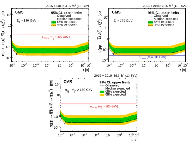
In the calorimeter search, the 95% confidence level (CL) upper limits onBσforeg (et) pair pro-duction for combined 2015 and 2016 data as a function of the particle’s lifetime τ are shown in Fig. 4, assuming Eg>130 GeV (meg−mχe0 '160 GeV or Et >170 GeV). In Fig. 5, the gluino and
top squark mass limits are shown, assumingB(eg → gχe
0) = B(
e
g → qqχe
0) = B(
et → tχe0) = 100%. We exclude gluinos with meg <1385 (1393) GeV that decay viaeg→gχe
0(
e
g→qqχe
0) and
top squarks with met <744 GeV at 95% CL for 10 µs<τ<1000 s.
Figure 6 shows the regions of the gluino (top squark) mass vs. neutralino mass plane excluded by the calorimeter search, for lifetimes between 10 µs and 1000 s. The borders of the regions are determined by the edge of the plateau in Fig. 2 and the gluino (top squark) mass limits.
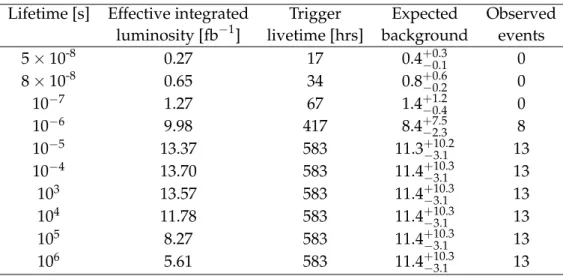
Table 7: Counting experiment results for different lifetimes in the calorimeter search with 2016 data.
Lifetime [s] Effective integrated Trigger Expected Observed
luminosity [fb−1] livetime [hrs] background events
5×10⁻⁸ 0.27 17 0.4+−0.30.1 0 8×10⁻⁸ 0.65 34 0.8+−0.60.2 0 10−7 1.27 67 1.4+−1.20.4 0 10−6 9.98 417 8.4+7.5 −2.3 8 10−5 13.37 583 11.3+−10.23.1 13 10−4 13.70 583 11.4+−10.33.1 13 103 13.57 583 11.4+−10.33.1 13 104 11.78 583 11.4+−10.33.1 13 105 8.27 583 11.4+10.3 −3.1 13 106 5.61 583 11.4+−10.33.1 13
Table 8: Counting experiment results for different lifetimes in the muon search with 2016 data.
Lifetime [s] Effective integrated Trigger Expected Observed
luminosity [fb−1] livetime [hrs] background events
5×10⁻⁸ 0.27 11 0.01±0.01 0 8×10⁻⁸ 0.64 34 0.03±0.02 0 10−7 1.27 68 0.06±0.05 0 10−6 9.95 422 0.36±0.29 0 10−5 13.34 581 0.49±0.39 0 10−4 13.67 589 0.50±0.40 0 1 13.67 589 0.50±0.40 0 103 13.55 589 0.50±0.40 0 104 11.75 589 0.50±0.40 0 105 8.26 589 0.50±0.40 0 106 5.61 589 0.50±0.40 0
gluinos and 400 GeV MCHAMPs are shown in Fig. 7 for combined 2015 and 2016 data. The
combined 2015 and 2016 95% CL upper limits onBσof gluino and MCHAMP pair production
as a function of mass are shown in Fig. 8, for lifetimes between 10 µs and 1000 s. Gluinos with masses between 400 and 980 GeV are excluded for lifetimes between 10 µs and 1000 s, assuming B(eg → qqχe 0 2)B(χe 0 2 → µ+µ−χe 0) = 100%, m e χ0 = 0.25megand mχe 0 2 = 2.5mχe0. MCHAMPs with
masses between 100 and 440 GeV and|Q| = 2e are excluded for lifetimes between 10 µs and
1000 s, assumingB(MCHAMP→µ±µ±) =100%.
9
Summary
A search has been presented for long-lived particles that stopped in the CMS detector after being produced in proton-proton collisions at a center-of-mass energy of 13 TeV at the CERN LHC. The subsequent decays of these particles to produce calorimeter deposits or muon pairs were looked for during gaps between proton bunches in the LHC beams. In the calorimeter (muon) search, with collision data corresponding to an integrated luminosity of 2.7 (2.8) fb−1 in a period of sensitivity corresponding to 135 (155) hours of trigger livetime in 2015 and to an integrated luminosity of 35.9 (36.2) fb−1 in a period of sensitivity of 586 (589) hours of trigger
17 [s] τ 7 − 10 10−5 10−3 10−1 10 103 105106 > 130 GeV g E = 800 GeV) g ~ (m theory σ 95% CL upper limits Observed Median expected 68% expected 95% expected ) [pb] 0 χ∼ g → g~( Β ) g~ g~ → (pp σ −2 10 1 − 10 1 10 2 10 (13 TeV) -1 2015 + 2016: 38.6 fb CMS [s] τ 7 − 10 10−5 10−3 10−1 10 103 105106 > 170 GeV t E = 800 GeV) t ~ (m theory σ 95% CL upper limits Observed Median expected 68% expected 95% expected ) [pb] 0 χ∼ t → t~( Β ) t~t~ → (pp σ 2 − 10 1 − 10 1 10 2 10 (13 TeV) -1 2015 + 2016: 38.6 fb CMS [s] τ 7 − 10 10−5 10−3 10−1 10 103 105106 160 GeV 0 χ∼ - m g ~ m = 800 GeV) g ~ (m theory σ 95% CL upper limits Observed Median expected 68% expected 95% expected ) [pb] 0 χ∼ q q → g~( Β ) g~ g~ → (pp σ10−2 1 − 10 1 10 2 10 (13 TeV) -1 2015 + 2016: 38.6 fb CMS > ~
Figure 4: The 95% CL upper limits onBσfor gluino and top squark pair production, using the
cloud model of R-hadron interactions, as a function of lifetime, for combined 2015 and 2016 data for the calorimeter search. We show gluinos that undergo a two-body decay (upper left), top squarks that undergo a two-body decay (upper right), and gluinos that undergo a
three-body decay (lower). The discontinuous structure observed between 10−7 and 10−5 s is due to
the increase of the number of observed events in the search window as the lifetime increases.
The theory lines assumeB =100%.
livetime in 2016, no excess above the estimated background has been observed. Cross section (σ) and mass limits have been presented at 95% confidence level (CL) on gluino (eg), top squark
(et), and multiply charged massive particle (MCHAMP) production over 13 orders of magnitude
in the mean proper lifetime of the stopped particle.
In the calorimeter search, combining the results from the 2015 and 2016 analyses and assuming a branching fraction (B) of 100% foreg→ gχe
0 (
e
g → qqχe
0), where
e
χ0 is the lightest neutralino, gluinos with lifetimes from 10 µs to 1000 s and m
e
g < 1385 (1393) GeV have been excluded,
for a cloud model of R-hadron interactions and for the daughter gluon energy Eg > 130 GeV
(meg−mχe
0 ' 160 GeV). Under similar assumptions, for the daughter top quark energy Et >
170 GeV andB(et→tχe
0) =100%, long-lived top squarks with lifetimes from 10 µs to 1000 s and
met < 744 GeV have been excluded. These are the first limits on stopped long-lived particles at 13 TeV and the strongest limits to date.
In the muon search, 95% CL upper limits on Bσ were set for combined 2015 and 2016 data.
For lifetimes between 10 µs and 1000 s, limits were set between 1 and 0.01 pb for gluinos with masses between 400 and 1600 GeV and for MCHAMPs with masses between 100 and 800 GeV
and charge |Q| = 2e. For lifetimes between 10 µs and 1000 s, gluinos with masses between
400 and 980 GeV have been excluded, assuming B(eg → qqχe
0 2)B(χe
0
2 → µ+µ−χe
[s] τ 7 − 10 10−5 10−3 10−1 10 103 105106 ) [GeV] ~t (m~g m 500 1000 1500 2000 2500 0 χ∼ t → t ~ , 0 χ∼ g → g ~ > 130 GeV g E > 170 GeV t E 95% CL upper limits observed t ~ / g ~ median expected t ~ / g ~ 68% expected t ~ / g ~ 95% expected t ~ / g ~ (13 TeV) -1 2015 + 2016: 38.6 fb CMS [s] τ 7 − 10 10−5 10−3 10−1 10 103 105106 [GeV] ~g m 500 1000 1500 2000 2500 0 χ∼ q q → g ~ 160 GeV 0 χ∼ - m g ~ m 95% CL upper limits Observed Median expected 68% expected 95% expected (13 TeV) -1 2015 + 2016: 38.6 fb CMS > ~
Figure 5: The 95% CL upper limits on the gluino and top squark mass, using the cloud model of R-hadron interactions, as a function of lifetime, for combined 2015 and 2016 data for the calorimeter search. We show gluinos and top squarks that undergo a two-body decay (left) and gluinos that undergo a three-body decay (right). The discontinuous structure observed between 10−7and 10−5s is due to the increase of the number of observed events in the search window as the lifetime increases.
22 23 24 25 26 27 28 29 30 31 ) [fb] 0χ∼ g → g ~ (Β ) g ~ g ~ → (pp σ 95% CL upper limit on 0 200 400 600 800 1000 1200 1400 1600 [GeV] g ~ m 0 200 400 600 800 1000 1200 1400 [GeV]0χ∼ m Kinematically forbidden < 1000 s τ s < µ 10 0 χ∼ g → g ~ > 130 GeV g E Observed Median expected 68% expected (13 TeV) -1 2015 + 2016: 38.6 fb CMS 30 32 34 36 38 40 42 44 0) [fb]χ∼ t → t~( Β ) t~t~ → (pp σ 95% CL upper limit on 0 100 200 300 400 500 600 700 800 [GeV] t ~ m 0 100 200 300 400 500 600 [GeV]0χ∼ m Kinematically forbidden < 1000 s τ s < µ 10 0 χ∼ t → t ~ > 170 GeV t E Observed Median expected 68% expected (13 TeV) -1 2015 + 2016: 38.6 fb CMS 22 23 24 25 26 27 28 29 ) [fb] 0χ∼ q q → g ~ (Β ) g ~g ~ → (pp σ 95% CL upper limit on 0 200 400 600 800 1000 1200 1400 1600 [GeV] g ~ m 0 200 400 600 800 1000 1200 1400 [GeV]0χ∼ m Kinematically forbidden < 1000 s τ s < µ 10 0 χ∼ q q → g ~ 160 GeV 0 χ∼ - m g ~ m Observed Median expected 68% expected (13 TeV) -1 2015 + 2016: 38.6 fb CMS > ~
Figure 6: The 95% CL upper limits in the neutralino mass vs. gluino (top squark) mass plane, for lifetimes between 10 µs and 1000 s, for combined 2015 and 2016 data for the calorimeter
search. The color map indicates the 95% CL upper limits onBσ. The mostly triangular region
defined by the black solid (dashed) line shows the excluded observed (expected) region. We show gluinos that undergo a two-body decay (upper left), top squarks that undergo a two-body decay (upper right), and gluinos that undergo a three-body decay (lower).
m e χ0 = 0.25meg, and mχe 0 2 = 2.5mχe0, whereχe 0
19 [s] τ 7 − 10 10−5 10−3 10−1 10 103 105106 = 1000 GeV) g ~ (m theory σ 95% CL upper limits Observed 68% expected 95% expected ) [pb] 0 χ∼ -µ + µ → 2 0 χ∼ ( Β ) 2 0 χ∼ q q → g ~ ( Β ) g ~ g ~ → (pp σ 1 − 10 1 10 (13 TeV) -1 2015 + 2016: 39.0 fb CMS [s] τ 7 − 10 10−5 10−3 10−1 10 103 105106 = 400 GeV) MCHAMP (m theory σ 95% CL upper limits Observed 68% expected 95% expected ) [pb] ± µ ± µ → (MCHAMP Β MCHAMP MCHAMP) → (pp σ 2 − 10 1 − 10 1 (13 TeV) -1 2015 + 2016: 39.0 fb CMS
Figure 7: The 95% CL upper limits on Bσ for 1000 GeV gluino (left) and 400 GeV MCHAMP
(right) pair production as a function of lifetime, for combined 2015 and 2016 data for the muon
search. The theory lines assumeB =100%.
[GeV] g ~ m 400 600 800 1000 1200 1400 1600 ) [pb] 0 χ∼ -µ + µ → 2 0 χ∼ ( Β ) 2 0 χ∼ q q → g ~ ( Β ) g ~ g ~ → (pp σ 10−2 1 − 10 1 10 2 10 95% CL upper limits s - 1000 s µ Observed, 10 s - 1000 s µ Median expected, 10 s - 1000 s µ 68% expected, 10 s - 1000 s µ 95% expected, 10 LO prediction (13 TeV) -1 2015 + 2016: 39.0 fb CMS [GeV] MCHAMP m 100 200 300 400 500 600 700 800 ) [pb] ±µ ±µ → (MCHAMP Β MCHAMP MCHAMP ) → (pp σ 3 − 10 2 − 10 1 − 10 1 10 95% CL upper limits s - 1000 s µ Observed, 10 s - 1000 s µ Median expected, 10 s - 1000 s µ 68% expected, 10 s - 1000 s µ 95% expected, 10 LO prediction (13 TeV) -1 2015 + 2016: 39.0 fb CMS
Figure 8: 95% CL upper limits onBσfor gluino (left) and MCHAMP (right) pair production as
a function of mass, for lifetimes between 10 µs and 1000 s, for combined 2015 and 2016 data for
lifetime hypothesis, MCHAMPs with masses between 100 and 440 GeV and|Q| =2e have been
excluded, assumingB(MCHAMP→µ±µ±) = 100%. These are the first limits obtained at the
LHC for stopped particles that decay to muons.
Acknowledgments
We congratulate our colleagues in the CERN accelerator departments for the excellent perfor-mance of the LHC and thank the technical and administrative staffs at CERN and at other CMS institutes for their contributions to the success of the CMS effort. In addition, we grate-fully acknowledge the computing centers and personnel of the Worldwide LHC Computing Grid for delivering so effectively the computing infrastructure essential to our analyses. Fi-nally, we acknowledge the enduring support for the construction and operation of the LHC and the CMS detector provided by the following funding agencies: BMWFW and FWF (Aus-tria); FNRS and FWO (Belgium); CNPq, CAPES, FAPERJ, and FAPESP (Brazil); MES (Bulgaria); CERN; CAS, MoST, and NSFC (China); COLCIENCIAS (Colombia); MSES and CSF (Croatia); RPF (Cyprus); SENESCYT (Ecuador); MoER, ERC IUT, and ERDF (Estonia); Academy of Fin-land, MEC, and HIP (Finland); CEA and CNRS/IN2P3 (France); BMBF, DFG, and HGF (Ger-many); GSRT (Greece); OTKA and NIH (Hungary); DAE and DST (India); IPM (Iran); SFI (Ireland); INFN (Italy); MSIP and NRF (Republic of Korea); LAS (Lithuania); MOE and UM (Malaysia); BUAP, CINVESTAV, CONACYT, LNS, SEP, and UASLP-FAI (Mexico); MBIE (New Zealand); PAEC (Pakistan); MSHE and NSC (Poland); FCT (Portugal); JINR (Dubna); MON, RosAtom, RAS, RFBR and RAEP (Russia); MESTD (Serbia); SEIDI, CPAN, PCTI and FEDER (Spain); Swiss Funding Agencies (Switzerland); MST (Taipei); ThEPCenter, IPST, STAR, and NSTDA (Thailand); TUBITAK and TAEK (Turkey); NASU and SFFR (Ukraine); STFC (United Kingdom); DOE and NSF (USA).
Individuals have received support from the Marie-Curie program and the European Research Council and Horizon 2020 Grant, contract No. 675440 (European Union); the Leventis Foun-dation; the A. P. Sloan FounFoun-dation; the Alexander von Humboldt FounFoun-dation; the Belgian Fed-eral Science Policy Office; the Fonds pour la Formation `a la Recherche dans l’Industrie et dans l’Agriculture (FRIA-Belgium); the Agentschap voor Innovatie door Wetenschap en Technologie (IWT-Belgium); the Ministry of Education, Youth and Sports (MEYS) of the Czech Republic; the Council of Science and Industrial Research, India; the HOMING PLUS program of the Foun-dation for Polish Science, cofinanced from European Union, Regional Development Fund, the Mobility Plus program of the Ministry of Science and Higher Education, the National Science Center (Poland), contracts Harmonia 2014/14/M/ST2/00428, Opus 2014/13/B/ST2/02543, 2014/15/B/ST2/03998, and 2015/19/B/ST2/02861, Sonata-bis 2012/07/E/ST2/01406; the National Priorities Research Program by Qatar National Research Fund; the Programa Severo Ochoa del Principado de Asturias; the Thalis and Aristeia programs cofinanced by EU-ESF and the Greek NSRF; the Rachadapisek Sompot Fund for Postdoctoral Fellowship, Chulalongkorn University and the Chulalongkorn Academic into Its 2nd Century Project Advancement Project (Thailand); the Welch Foundation, contract C-1845; and the Weston Havens Foundation (USA).
References
[1] S. Dimopoulos, M. Dine, S. Raby, and S. D. Thomas, “Experimental signatures of low-energy gauge mediated supersymmetry breaking”, Phys. Rev. Lett. 76 (1996) 3494,
References 21
[2] H. Baer, K.-M. Cheung, and J. F. Gunion, “A heavy gluino as the lightest supersymmetric particle”, Phys. Rev. D 59 (1999) 075002, doi:10.1103/PhysRevD.59.075002, arXiv:hep-ph/9806361.
[3] T. Jittoh, J. Sato, T. Shimomura, and M. Yamanaka, “Long life stau in the minimal supersymmetric standard model”, Phys. Rev. D 73 (2006) 055009,
doi:10.1103/PhysRevD.73.055009, arXiv:hep-ph/0512197. [Erratum: doi:10.1103/PhysRevD.87.019901].
[4] M. Fairbairn et al., “Stable massive particles at colliders”, Phys. Rept. 438 (2007) 1,
doi:10.1016/j.physrep.2006.10.002, arXiv:hep-ph/0611040.
[5] M. J. Strassler and K. M. Zurek, “Echoes of a hidden valley at hadron colliders”, Phys. Lett. B 651 (2007) 374, doi:10.1016/j.physletb.2007.06.055,
arXiv:hep-ph/0604261.
[6] A. Arvanitaki et al., “Astrophysical probes of unification”, Phys. Rev. D 79 (2009) 105022, doi:10.1103/PhysRevD.79.105022, arXiv:0812.2075.
[7] N. Arkani-Hamed and S. Dimopoulos, “Supersymmetric unification without low energy supersymmetry and signatures for fine-tuning at the LHC”, JHEP 06 (2005) 073,
doi:10.1088/1126-6708/2005/06/073, arXiv:hep-th/0405159.
[8] A. Arvanitaki, N. Craig, S. Dimopoulos, and G. Villadoro, “Mini-split”, JHEP 02 (2013) 126, doi:10.1007/JHEP02(2013)126, arXiv:1210.0555.
[9] A. Arvanitaki et al., “Stopping gluinos”, Phys. Rev. D 76 (2007) 055007,
doi:10.1103/PhysRevD.76.055007, arXiv:hep-ph/0506242.
[10] P. W. Graham, K. Howe, S. Rajendran, and D. Stolarski, “New measurements with stopped particles at the LHC”, Phys. Rev. D 86 (2012) 034020,
doi:10.1103/PhysRevD.86.034020, arXiv:1111.4176.
[11] CMS Collaboration, “Search for decays of stopped long-lived particles produced in proton-proton collisions at√s=8 TeV”, Eur. Phys. J. C 75 (2015) 151,
doi:10.1140/epjc/s10052-015-3367-z, arXiv:1501.05603.
[12] D0 Collaboration, “Search for stopped gluinos from p ¯p collisions at√s=1.96 TeV”, Phys. Rev. Lett. 99 (2007) 131801, doi:10.1103/PhysRevLett.99.131801,
arXiv:0705.0306.
[13] CMS Collaboration, “Search for stopped long-lived particles produced in pp collisions at√
s =7 TeV”, JHEP 08 (2012) 026, doi:10.1007/JHEP08(2012)026,
arXiv:1207.0106.
[14] CMS Collaboration, “Search for stopped gluinos in pp collisions at√s=7 TeV”, Phys.
Rev. Lett. 106 (2011) 011801, doi:10.1103/PhysRevLett.106.011801,
arXiv:1011.5861.
[15] ATLAS Collaboration, “Search for decays of stopped, long-lived particles from 7 TeV pp collisions with the ATLAS detector”, Eur. Phys. J. C 72 (2012) 1,