Medical Image Segmentation Based on AIFs

Medical Image Segmentation Based on AIFs

Doctoral Thesis in Computer Science

Telmo Rui Dias Bento

Supervisor: Professor Doutor Pedro Alexandre Mogadouro do Couto

Co- supervisor: Professor Doutor Pedro José de Melo Teixeira Pinto

Medical Image Segmentation Based on AIFs

Doctoral Thesis in Computer Science

Telmo Rui Dias Bento

Supervisor: Professor Doutor Pedro Alexandre Mogadouro do Couto

Co-supervisor: Professor Doutor Pedro José de Melo Teixeira Pinto

Jury composition:

I

Na presente tese é introduzida uma nova abordagem para realizar a delineação de tumores em imagens obtidas por tomografia por emissão de positrões (PET). Assim, apresentar-se-á uma nova metodologia iterativa baseada em segmentação por threshold global utilizando Conjuntos Difusos Intuicionistas de Atanassov (A-IFSs) e funções de dissimilaridade restrita.

No desenvolvimento desta metodologia, foram propostos dois critérios de paragem do algoritmo iterativo, tendo ainda sido criado diferentes implementações para cada uma das soluções.

O Índice Intuicionista Difuso de Atanassov é utilizado como o grau de incerteza no processo de associação, para decidir se um pixel de uma imagem pertence ao fundo ou ao objeto/tumor da imagem, utilizando a entropia de forma idêntica à aplicação da entropia difusa nos algoritmos difusos de segmentação existentes.

Foram implementados dois algoritmos principais utilizando cada um dos critérios de paragem propostos. Foram analisadas opções para cada um dos algoritmos de modo a melhorar a deteção dos limites, com o objetivo de facilitar a pesquisa do limite ideal para o delineamento de tumores em imagens PET. Finalmente, foi proposto um critério de homogeneidade a utilizar no algoritmo iterativo para delinear tumores em imagens PET.

Foram realizados diversos testes de análise do algoritmo em causa, bem como comparação com outras metodologias existentes. Os resultados experimentais obtidos indicam, que o método desenvolvido apresenta melhor desempenho que os métodos existentes.

III

This thesis introduces a new approach to perform tumor delineation in Positron Emission Tomography (PET) images. A new iterative methodology based on global threshold segmentation using Atanassov’s Intuitionistic Fuzzy Sets (A-IFSs) and restricted dissimilarity functions.

In the development of this methodology, two stopping criteria for the iterative algorithm were proposed, and different implementations were created for each of the solutions.

The Intuitionistic Fuzzy Index of Atanassov is used as the degree of unknowledge of an expert to decide if a pixel of an image belongs to the background or to the object/tumor of the image, using the entropy the same sense as fuzzy entropy is used in the existing fuzzy algorithms.

Two main algorithms were implemented using each of the proposed stopping criteria. Several options were analyzed for each algorithm to improve the delineation, to improve the search for the optimal threshold for tumor delineation in PET images. Finally, it was proposed a homogeneity criterion to be used in the iterative algorithm to delineate tumors in PET images.

Several tests of analysis of the algorithm were performed, as well as a comparison with other existing methodologies. The obtained experimental results indicate that the developed method outperforms the existing methods.

Key Words: PET, Medical Image, Thresholding, Segmentation, Fuzzy Logic,

V

I'll like to thank my family and friends for pushing me and encourage me to don’t give up during these last’s years. I am especially thankful to my girlfriend Rita Araújo who suffered the most from my time spending, and sometimes my deepest frustrations during all this process, without her help and comprehension I would never get this far and be here.

I would like to express my deep and sincere gratitude to my supervisors, Professor Pedro Couto, Ph.D., and Professor Pedro Melo-Pinto, Ph.D., who had an important role during all my academic journey. They have been unstoppable trying to motivate me and keep challenging me to pass through the different stages, since my first academic year. Once more, thank you very much for all the time and dedication.

VII

Resumo ... I

Abstract ... III

Acknowledgements ... V

List of Figures ... XI

List of Tables... XIII

Acronyms ... XV

1. Introduction ... 1

2. Categorization of Positron Emission Tomography ... 5

2.1 Introduction ... 6

2.2 Description ... 7

2.3 Physical Principles of PET Imaging ... 7

2.4 Positron Emitting Radiopharmaceuticals ... 9

2.5 Technology for PET/CT ...10

2.6 Clinical Application of PET ...11

2.7 Conclusion ...12

3. Image Segmentation ... 15

3.1 Introduction ...15

3.2 Image Segmentation Techniques ...17

3.2.1 Edge-Based Image Segmentation ...18

3.2.2 Region-Based Image Segmentation ...25

3.2.3 Threshold-Based Image Segmentation ...29

VIII

Tomography ... 43

3.3.3 Edge-Based Segmentation Techniques in Positron Emission Tomography ... 47

3.3.4 Stochastic Methods in Positron Emission Tomography ... 47

4 Fuzzy Logic in Image Segmentation ... 55

4.1 Fuzzy Logic Theory ... 55

4.1.1 Fuzzy Sets ... 56

4.2 Atanassov’s Intuitionistic Fuzzy Sets - (A-IFSs) ... 61

4.2.1 Distances between A-IFS ... 63

4.2.2 Entropy on A-IFSs ... 64

4.3 General Framework for A-IFSs based Image Threshold ... 66

5 A-IFSs unsupervised Segmentation for PET Delineation ... 69

5.1 Fuzzy Logic based Image Thresholding using A-IFSs ... 70

5.2 PET image Iterative Thresholding using A-IFSs ... 73

5.2.1 Amplitude Stopping Criteria A-IFSs Segmentation (ASCAS) .. 75

5.2.2 Positional Stopping Criteria A-IFSs Segmentation (PSCAS)... 77

5.2.3 ASCAS extended and PSCAS extended ... 78

5.3 Using the K value to perform tumor delineation on PET images 80 5.4 Achieving tumor delineation with PET image Iterative Thresholding using A-IFSs... 84

6 Tests and Results ... 89

6.1 PET images segmentation obtained with ASCAS and PSCAS ... 90

6.2 PET images segmentation obtained with ASCASe and PSCASe ... 95

6.3 Tumor delineation in PET image with Iterative Thresholding using A-IFSs ... 101

IX

7. Conclusions and Future Work ... 111

Bibliography ... 115

APPENDIX ... 143

XI

Figure 1 - The principles of PET imaging shown schematically [15]. ... 8

Figure 2 - (A) Sagittal PET image, (B) sagittal reformatted CT image, and (C) PET/CT image with CT component in grayscale and PET image in red temperature color scale.[45] ...10

Figure 3 - Illustration of the major PET/CT scanner components.[45] ...11

Figure 4 – 3 x 3 Sobel masks. ...19

Figure 5 – 3 x 3 Laplacian mask ...20

Figure 6 – Blood cells image and Image Histogram ...30

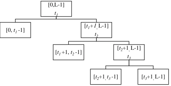
Figure 7 – Abutaleb’s 2-D gray level histogram with threshold vector (𝑡, 𝑡 ) ...37

Figure 8 – Thresholding methods for PET images. ...39

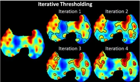
Figure 9 - The segmentation results at each iteration ...43

Figure 10 – Computational Process ...74

Figure 11 – Original image, ground truth, and segmentation with ASCAS and PSCAS ...78

Figure 12 – Image original, ground truth and segmented with ASCASe and PSCASe ...79

Figure 13 - Evolution of Homogeneity in four examples of PET images through the iterations ...87

Figure 14 – Examples of images from different patients ...89

Figure 15 - a,b,c - Examples of original images, d,f,g - Corresponding expert’s delineation ...90

Figure 16 - a - Algorithm comparison with 𝐼𝑜𝑈, b - Algorithm comparison with pixel accuracy and c - Algorithm comparison with 𝑆𝑤. ... 109

XIII

Table 1 - Physical properties of some positron-emitting radionuclides [36], [38] .. 9

Table 2 – PET 1 processed with different K values with ASCAS ...82

Table 3 - PET 3 processed with different K values with ASCAS ...82

Table 4 - PET 10 processed with different K values with ASCAS ...83

Table 5 - PET 13 processed with different K values with ASCAS ...83

Table 6 – Homogeneity values (𝐻) ...86

Table 7 – ASCAS and PSCAS results ...92

Table 8 – ASCAS and PSCAS number of thresholds and thresholds values ...94

Table 9 - ASCASe and PSCASe results ...97

Table 10 – Algorithm 3 and Algorithm 4 number of thresholds and thresholds values ...99

Table 11 - Tumor delineation in PET image with iterative thresholding using A-IFSs results ... 103

Table 12 – Fixed thresholds 𝐼𝑜𝑈 results. ... 106

XV

AIFs Atanassov’s Intuitionistic Fuzzy Sets ANN Artificial Neural Network

AP Affinity Propagation

ARG Adaptive Region Growing

ASCAS Amplitude Stopping Criteria A-IFSs Segmentation

CT Computerized Tomography

FCM Fuzzy C-Means

FDG Fluorodeoxyglucose

FLAB Fuzzy Locally Adaptive Bayesian

FWHM Full Width at Half Maximum

GMM Gaussian Mixture Models

ITM Iterative Threshold Method

KDE Kernel Density Estimation

NSCLC Non-Small-Cell Lung Carcinoma

PDE Partial Differential Equation

PET Positron Emission Tomography

PMF Probability Mass Function

PSCAS Positional Stopping Criteria A-IFSs Segmentation

PVE Partial Volume Effect

ROI Region Of Interest

RW Random Walk

SBR Source-to-Background Ratio

1. Introduction

The segmentation of digital images is the procedure to partitioning an image into disjoint parts, regions, classes, or subsets to the extent that every part must fulfill an unmistakable and very characterized property and attribute. Image segmentation is an important step towards the analysis of image information. In this way, the importance of image segmentation can’t be neglected because it is applied in almost every field of science, for example, satellite imaging, computer vision, biometrics, medical images and others [1]–[7].

In this work, we will use image segmentation based on Atanassov’s Intuitionistic Fuzzy Sets (A-IFSs) to detect and delineate tumors in Positron Emission Tomography (PET) images.

Positron Emission Tomography or PET is a technique for the imaging of physiological processes in humans. This technique presents the distribution of a radioactive emitter monitored by surrounding detectors. With the aid of mathematical algorithms, the distribution of the marker reconstructs the image.

PET is heavily used in medicine, biology, neurology and pharmaceutical research measuring brain activity, blood or glucose. Several interdisciplinary initiatives were merged within a running PET system, ranging from physics, communication technology, electrical engineering, and image reconstruction to ensure its application in medicine. In this way, PET has become an indispensable tool to ensure accurate and early diagnosis, and for the treatment of cancer patients, namely in cancer illness [8]–[15].

PET images are known for their high sensitivity and low spatial resolution. Moreover, PET images suffer from noise caused by random and scattered coincidences and have low signal-to-noise ratios. With these conditions, the difficulties for a successful image segmentation increase [8], [16]–[25].

In this work, PET images will be processed using fuzzy logic algorithms to partition the image sections and use a selected criterion to delineate the tumor region on each image.

The main contributions of this thesis are:

• Extended of the A-IFSs multilevel threshold-based methodology with two stopping criteria.

• Unsupervised A-IFSs based segmentation methodology for PET image tumor delineation.

Other contributions:

• Study of different variants of the original algorithm

• Study of the regularizing factor K

The thesis is organized as follows:

In chapter 2 we analyze PET as a technique for the imaging of physiological processes in humans. We present the concept of PET images, their physical principles, the radiopharmaceuticals need to create the images, the technologies, and the procedures to obtain the images and the clinical applications of these images.

In chapter 3 we present research regarding the image segmentation field over the last years, and the diverse types of segmentation techniques that have been proposed in the literature, each one of them based on a specific methodology to classify the regions. Also, address the techniques proposed in the literature used for PET image segmentation.

In chapter 4, we present a brief review on fuzzy logic theory and its main concepts, describe the main concepts of A-IFSs and its applications, namely to image segmentation and the concept of entropy on A-IFSs.

In chapter 5, we introduce the IFSs algorithm, the extended multilevel IFSs image segmentation using different stopping criteria and an unsupervised A-IFSs based segmentation methodology for PET image tumor delineation.

In Chapter 6, experimental results and comparisons, with other existing algorithms, are presented and discussed.

In Chapter 7, we present the conclusions taken from this work, and we foresee some future directions this work may take.

2. Categorization of Positron

Emission Tomography

The objective of this chapter is to analyze Positron Emission Tomography or PET as a technique for physiological processes imaging in humans. This technique presents the distribution of a radioactive emitter and monitored by surrounding detectors in a noninvasive way. The distribution of the marker reconstructs the image using mathematical algorithms. PET has become an indispensable tool to ensure accurate and early diagnosis and for the treatment of cancer patients, namely in cancer illness.

PET is mostly used in medicine, biology, neurology, and pharmaceutical research. Several interdisciplinary initiatives were merged within a running PET system, ranging from physics, communication technology, electrical engineering and image reconstruction to the application in medicine. Thus, modern physicists need to understand not only the underlying physics but also how the system functions and operations.

Positron emission tomography imaging is recognized as a powerful metabolic imaging technique which applies the best radiopharmaceutical we have ever used [18_{F]-fluorodeoxyglucose (FDG) [15], [26], [27]. In addition, in the content} of sensitivity, it yields images that the importance of which can be appreciated by non-nuclear medicine clinicians and has an enormous clinical impact. The recognition that functional imaging modalities, such as PET, may provide a great improvement in earlier diagnosis and more accurate staging than the conventional anatomic imaging. An oncologist with access to a good PET imaging service can very quickly appreciate its value. In the context of clinical reporting sessions, the contributes of PET use can be appreciated. To patient management, the new information provided by the PET images proves to be a useful tool, with significant effects. Although PET offers an extensive list of different radiopharmaceuticals, or molecular probes, to image different aspects of physiology and tumor biology, the currently most used PET tracer is the fluorinated analog of glucose, known as FDG.

The increased uptake of glucose in malignant cells has been well known for many years [28], and although FDG is not a specific probe for cancer, it can be a useful property when identifying and staging disease by a scan of the whole body.

2.1 Introduction

Nowadays, there is an extensive quantity of data evaluating the impact of PET on patient management. Studies shows that the results obtained from PET images produces a major change in patient management, with changes in more than 25% of patients, and in some cases it is possible to reach changes at 40% of patients management [29]. Examples include changes in surgical treatment for non-small cell lung cancer, the staging, and treatment of lymphoma. For instance, it is possible to avoid inappropriate surgery and to enable potentially curative resection.

The combination of PET/CT instrumentation is an important evolution in imaging technology. The first prototype of the computed tomography (CT) scanner was presented in the early 1970s, and tomographic imaging has made significant contributions to the diagnosis and staging of diseases ever since. Both CT scanners and PET scanners have their strengths. CT scanners obtain the anatomy image with high spatial resolution, but the accurate location of the node may be an issue or a weakness. PET scanners can detect a functional abnormality in a normal-sized lymph node. Still, for PET scanners, it is difficult or even impossible to achieve the accurate localization of the node. So the evolution required the use of CT and PET as one single integrated device [30], being the first combined PET/CT prototype scanner completed in 1998 [31], and clinical evaluation began in June of that year. The initial studies with the prototype [13], [32]–[34] demonstrated a number of significant advantages of PET/CT. Functional abnormalities could now be accurately localized, that normal benign uptake of a nonspecific tracer such as FDG could be distinguished from uptake resulting from disease, and that confidence in reading both the PET and the CT increases significantly by having the anatomic and Positron Emission Tomography functional images routinely available and accurately aligned for every patient.

2.2 Description

Positron Emission Tomography (PET) is a nuclear medicine diagnostic imaging exam. Nuclear medicine exams use small amounts of radioactive material, known as radiopharmaceuticals, that are usually injected into the patient's bloodstream, being occasionally swallowed or inhaled. The radiopharmaceutical most common used in PET scanning is the FDG. FDG is a form of sugar and is avidly absorbed by tumor cells because these use sugar for growth. However, metabolically active normal tissues like the brain, as well as benign conditions such as inflammation, also take up FDG. Imaging exams, such as plain radiography, ultrasound, computed axial tomography (CAT or CT) and magnetic resonance imaging (MRI) are routinely used to provide information on the shape and size of anatomical structures and this information is used for both diagnosis and treatment decision-making. However, PET scanning can provide information on the extent of metabolic activity of abnormal tissues, such as cancer, and it has the potential to identify areas of abnormal metabolic activity before there is a distortion of the anatomy.

2.3 Physical Principles of PET Imaging

PET scanning is a process involving multiple steps. Firstly, a suitable molecular probe is selected and produced, then the probe is administrated to the patient, finally the imaging of the distribution of the probe in the patient. Positron emitters are neutron deficient isotopes that reach stability through the nuclear transmutation of a proton into a neutron. This process involves the emission of a positive electron, or positron (β) and an electron neutrino (𝑣𝑒) as shown in Figure 1-a. The emitted positron energy spectrum depends on the specific isotope, with typical endpoint energies varying from 0.6 MeV for 18_{F up to 3.4 MeV for 82Rb.} The positron loses energy after emission as a result of the interactions with the surrounding tissue, until it annihilates with an electron, Figure 1-b. The density of the surrounding tissue and the energy with which the positron is emitted affect the range that the positron can achieve. The two annihilation photons are detected in coincidence, it is important to have in consideration that they are emitted in

approximately opposite directions. In the example used, 𝜏 is the electronic coincidence time window, the coincidence is defined by two photons that are registered within a time interval of 2𝜏 ns, where [15].

Figure 1 - The principles of PET imaging shown schematically [15].

Positron emitters such as 18_{F are used to label substrates such as} deoxyglucose (DG) to create the radiopharmaceutical FDG (Figure 1-c). The radioactive tag is incorporated into the organ of interest through the metabolism of the pharmaceutical and transported by the human circulatory system. For FDG, glucose utilization is the main significant metabolic process. The images shown in Figure 1-f are maps of FDG accumulation throughout the body, reflecting glucose utilization by the different tissues.

The principles of PET are the interactions through a metabolic process of the pharmaceutical with the body tissue. The radionuclide allows that interaction to be followed, mapped, and measured [15].

2.4 Positron Emitting Radiopharmaceuticals

The most important radionuclides are 15_O, 13_N, 11_{C, and} 18_{F being their} half-life shown in Table 1. For clinical applications, 18_{F, due to the widespread use of} FDG, is of greatest importance in oncology [35]–[37]. The maximum energy of the positron from the decay of 18_{F is 0.633 MeV, with a mean range of 0.6 mm. With} these values, it is a nuclide with favorable properties for considerable good resolution PET imaging [15].

Radionuclide Half-Life (min) Maximum positron energy (MeV)

Maximum linear range (mm)

11_{C 20.4 0.96 5.0}

15_{O 9.9 1.19 5.4}

13_{N 2.1 1.72 8.2}

18_{F 110 0.633 2.4}

Table 1 - Physical properties of some positron-emitting radionuclides [36], [38]

Carbon, nitrogen, and oxygen are essential atoms to most physiological processes. Also, Fluorine has been found a useful radionuclide to label biologically important molecules. One of the most challenging problems found was the labeling of pharmaceuticals for medical use with positron-emitting nuclides. In 1980, a list of approximately 30 compounds labeled with positron-emitting radionuclides was published [39].

In this work, we will explore PET image in oncology and this following 18_F is the most accurate and non-invasive method to detect and stage tumors, as shown in the literature [35], [40]–[43]. It represents a significant improvement in terms of treatment planning and avoiding unnecessary treatment and its associated morbidity and costs. The establishment of diagnostic accuracy and positive impact on patient management are evidence of the gains obtained through the use of PET clinical practice [36], [42], [44].

2.5 Technology for PET/CT

Mutual positron emission tomography and computed tomography (PET/CT) scanners combine two unique techniques to provide unsurpassed patient diagnostic capabilities. PET/CT plays a major role in medicine for in vivo imaging in oncology, cardiology, neurology, psychiatry, and it is considered as a significant advance in imaging technology and patient care [15], [34], [45], [46].

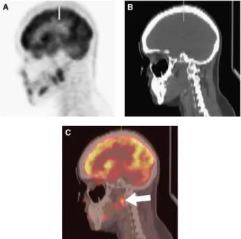
The first PET/CT scanner was introduced in 1998 through a collaboration of the National Cancer Institute, CTI PET Systems (Knoxville, Tennessee), and the University of Pittsburgh [31]. This scanner was constructed from independent, previously developed CT and PET scanners. The combination of independent components remains the standard for scanner design today. PET/CT scanners provide a simple solution to the localization task. Figure 2 presents a PET/CT scan with the separate PET (Figure 2-A) and CT (Figure 2-B) sagittal head images and the combined PET/CT image (Figure 2-C). This hardware alignment of the images reveals that a tumor is located in the right retropharyngeal space, an interpretation challenging to make based on a CT alone [45].

Figure 2 - (A) Sagittal PET image, (B) sagittal reformatted CT image, and (C) PET/CT image with CT component in grayscale and PET image in red temperature color

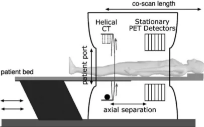
In a broad sense, a PET/CT scanner consists of three main components: a PET scanner, a CT scanner, and a patient bed. Currently, all of the major commercial systems, as GE Healthcare, Siemens Healthcare, and Philips Healthcare consist of a PET component with independent detectors, electronics, and acquisition system, and a CT component with its own set of independent modules.

Figure 3 shows the components of a typical PET/CT scanner. A single bed moves axially into the scanner while the patient receives first a CT scan and then a PET scan.

Figure 3 - Illustration of the major PET/CT scanner components.[45]

2.6 Clinical Application of PET

Nowadays, clinical PET imaging, using almost exclusively FDG, is being used in three critical areas of clinical diagnosis and management: cardiology and cardiac surgery; neurology and psychiatry; cancer diagnosis and management [27], [47].

In clinical cardiology, FDG-PET can identify the so-called "hibernating myocardium”. FDG-PET imaging of atherosclerosis to detect patients at risk of stroke is also feasible and can help test the efficacy of novel anti-atherosclerosis therapies [48].

Neurology and psychiatry involve all the process of management of brain tumors, the pre-surgical workup of patients with epilepsy resistant to medical therapies, and the identification of tumors causing paraneoplastic syndromes. Additionally, for the early diagnosis and differential diagnosis of dementia, PET has proved to outperform all other methods for [27], [47].

In cancer diagnosis and management, 18_{F-FDG PET proved to be the most} accurate non-invasive method to detect and identify stage tumors [35], [40]–[43]. PET has the potential to highly improve the ability to manage cancer patients and is making major contributions to the understanding of cancer biology and the development of new therapies [36].

2.7 Conclusion

PET is used in radiation oncology, at several stages of the treatment. Before the treatment, it serves in the disease diagnosis and staging. PET images can also be involved in the treatment planning, during the treatment, PET can assess the tumor response, and after the treatment, PET can be used in the patient follow-up, to detect recurrences. Despite the essential uses of PET in oncology, it has some throwbacks since the PET images don´t preserve spatial references and have poor quality and are very sensitive to noise.

Thus, the accuracy of automatic target delineation is directly conditioned by image quality [49], [50]. Increasing the acquisition duration of the tracer dose can contribute to improving the signal-to-noise ratio of the image. These requirements must naturally be put in balance with patient comfort and financial costs. Simple moves like when the patient breathes, and other movements should be carefully addressed. Motion blur significantly complicates the delineation task. Image

reconstruction should be achieved with modern iterative algorithms, which are less prone to artifacts. Beside the signal-to-noise ratio, the resolution is another important factor in the quality of delineation. The lower the resolution is, the stronger the object edges are blurred and distorted, making accurate delineation very challenging. Although the underlying physical process of PET limits the resolution of the images, the reconstruction has a non-negligible impact. For image segmentation, reconstruction protocols should avoid heavy smoothing and include resolution recovery techniques. Obtaining higher quality images usually increases the reconstruction time. If properly designed, delineation techniques can cope with noisy images, although they are not visually pleasant [51].

Perform image segmentation for PET images is a hard task because of the nature of the images. The noise, low resolution and the blurred edges of the PET images in addition to the high precision needed in the segmentation, increase the complexity of the problem.

3. Image Segmentation

3.1 Introduction

Image segmentation is one of the most studied and imperative areas in Computer Vision and one of the essential steps in image analysis techniques. Image segmentation refers to the procedure of dividing a picture into various portions, being a strategy to characterize the pixels of an image. This procedure assigns a value to every image pixel in order to make it simple to separate between various portions of any image. Briefly, image segmentation is the procedure of partitioning an image into disjoint parts, regions, classes, or subsets to achieve an unmistakable and very characterized property and attribute to every part. Image segmentation is an important step towards a proper analysis of image information. The importance of image segmentation can’t be neglected because it is used in almost every field of science, for example, removing noise, satellite imaging, computer vision, biometrics, medical images and other.

Herewith, it is unrealistic to identify a single method for perfect image segmentation, since each image has its own different type and characteristics. Also, it is hard to discover a segmentation method for a specific kind of image, since the method applied to one image may not be suitable to other images. There is broad research done in image segmentation over time and, as a result of the multidisciplinary and the diverse applications of image segmentation, there are many sorts of segmentation techniques proposed in the literature, every one of them under a specific innovation to classify regions. Subsequently, there is no standard technique for image segmentation. Image segmentation can be performed in color or grayscale images. Color image segmentation algorithms are usually an extension of the segmentation algorithms for the grayscale images, since color images work with three matrices of intensities values, in case of RGB images, instead with only one matrix of intensities values for grayscale. Considering that PET images are grayscale images, in this work we direct our studies to grayscale segmentation algorithms. Generally, segmentation algorithms for grayscale images are based on one of two basic properties of image intensity

values: discontinuity and similarity. In the first category, the approach is to partition an image based on abrupt changes in intensity, such as edges/boundaries. The second category is based on partitioning an image into regions that are similar according to a set of predefined criteria. For each category, and due to the multidisciplinary and the diverse applications of image segmentation, there is an extensive collection of methods. The most popular image segmentation systems include Edge-based segmentation, Fuzzy theory-based segmentation, Partial Differential Equation (PDE) based segmentation, Artificial Neural Network (ANN) based segmentation, threshold-based image segmentation, and Region-based image segmentation.

Image segmentation in PET images is challenging due to poor resolution and low signal-to-noise ratio inherent. Nevertheless, accurate tumor segmentation from PET images plays a crucial role in clinical diagnosis and in assessing therapy response. Since PET images identify damaged tissues, where they are identified by the different levels of intensities recorded in PET images, the image segmentation will play an important role in automating or assisting the identification of these regions. As the image segmentation is intended to divide the image into different subsets, which will allow a better analysis of the image, performed correctly, this will provide recognition and delineation of the damaged tissue, producing important information about the size and edges of the damaged tissue. Also, in order to have spatial location it is necessary to have CT images to give complementary spatial information since it is impossible to obtain the spatial location from the PET images. This information is critical for clinical diagnosis, therapy and follow-up of the tumors.

Several efforts have been made for creating new segmentation algorithms to address the diverse issues regarding manual delineation, like time-consuming, intensive labor and operator dependent, with high inter- and intra-observer inconstancy. Automated proposals, such as fuzzy C-means, adaptive region growing, and dual-front active contour, have been proposed for PET image segmentation. However, these methodologies are frequently restricted to simulations and specific sorts of tumors, e.g., non-small cell lung carcinoma (NSCLC) and head-and-neck tumor. These fully automated approaches are unable

to provide sufficiently accurate and robust PET tumor segmentation for small and/or low-contrast tumors.

In this following chapter, we will present different image segmentation techniques, explore general and specific methods used in PET images. The general methods are presented in three categories: edge-based, region-based and threshold-based methods; for PET image segmentation methods we add the stochastic methods category.

The method developed is a threshold-based category. Threshold techniques in positron emission tomography can be distinguished into three categories, namely, fixed thresholding, adaptive thresholding, and iterative thresholding.

3.2 Image Segmentation Techniques

Image segmentation involves two processes: recognition and delineation. The Recognition process embraces the determination of the pixels that belong to the object and on the other hand, to distinguish these pixels from other object-like entities in the image. Trough the process of delineation, it is possible to define the spatial extent of the object region in the image.

In recent years deep learning based approaches have been used successfully in image segmentation. However, it has some downsides like the need of extensive training samples and less accurate delineation [21]. Considering that tumor delineation for PET images needs an accurate delineation, these methods are usually used for general segmentation purposes, but aren’t appropriate for more precise delineation in this case [52]–[56].

3.2.1 Edge-Based Image Segmentation

An edge refers to the image pixels that belong to the transition between object and background or various objects. In edge-based image segmentation the methods detect the boundaries of the objects looking for the brightness transitions between regions.

Roberts [57] and Prewitt [58] initiated the use of this technique with their previous work. Thereafter, various methods of edge detection have been suggested with two basic local approaches: first and second order differentiation.

Image edges are usually blurred, thus, instead of a sharp transition in the image, the blurred edges result in a “ramplike” transition. In such cases, the use of the first derivative magnitude has an important role in detecting the edges of an image, since its value is 0 in areas of constant gray levels, maximum in points of transition into and out of the ramp and constant along the ramp.

Edge and noise vary rapidly spatially and subsequently have critical high spatial frequency components. This makes the existence of noise in an image a problem for the operator, much due to any derivative operator that reacts well to the existence of an edge is probably going to react equally well to the existence of noise. Additionally, the second derivative is significantly more sensitive to the noise than the first one. One way to deal with noisy images is smoothing the image before applying the edge detector [59].

The gradient is commonly used to compute the first-order derivative, the second-order derivative is computed using the Laplacian.

First-order derivatives of an image 𝑄 are based on variations of the 2-D gradient being defined as follows:

∇𝑄 = [_𝐺𝐺𝑥 𝑦] = [ 𝜕𝑄 𝜕𝑥 𝜕𝑄 𝜕𝑦 ]

These derivatives are applied to an image convolving it with fixed size masks such as Roberts, Prewitt and Sobel masks. Sobel masks like the 3 × 3 masks shown in Figure 4 are among the most used in image gradient computations. The Sobel mask presents a weighting of local average measures at both sides of the central pixel, being these masks an improvement of the Roberts and Prewitt’s masks. The weighting factor introduced arouse interest in the study and optimization of several works, particularly in the Canny edge detector [60], [61]. Canny followed a list of three criteria to improve current methods of edge detection: (a) low error rate, (b) edge points well localized, (c) have only one response to a single edge. In compliance with these criteria, the Canny edge detector first smooths the picture by Gaussian convolution. At that point, a simple 2-D first derivative operator is applied to the smoothed image. The algorithm then tracks along the image and suppresses any pixel that is not at the maximum. The gradient array is now further reduced by hysteresis by means of two thresholds: 𝑡1 and 𝑡2 with 𝑡1 > 𝑡2. If the magnitude is below 𝑡2, the pixel is set to zero defining it as non-edge. If the magnitude is above 𝑡1, it is made an edge. Besides, if the magnitude is between the two thresholds, then it is set to zero unless there is a path from this pixel to a pixel with a gradient above 𝑡2. The good results achieved from the Canny edge detector, make it known to many as the optimal edge detector. 𝐺𝑦= [ −1 −2 −1 0 0 0 1 2 1 ] 𝐺𝑥 = [ −1 0 1 −2 0 2 −1 0 1 ]

Figure 4 – 3 x 3 Sobel masks.

The masks are used to obtain the values of the gradient components 𝐺𝑥 and 𝐺𝑦. The masks in Figure 4 only give results for horizontal and vertical edges, they can be easily adapted to respond along with diagonal directions.

The 2-D Laplacian of an image 𝑄 is a second-order derivative defined as follows: ∇2_{𝑄 =}𝜕 2_𝑄 𝜕2_𝑥+ 𝜕2𝑄 𝜕2_𝑦

Laplacian Masks like the 3 x 3 mask in Figure 5 are convolved with the image to obtain the second derivative of the image.

[

−1 −1 −1 −1 8 −1 −1 −1 −1 ]

Figure 5 – 3 x 3 Laplacian mask

The Laplacian isn’t typically used in its original form, because as it is a second derivate, it produces double edges, the transition in and out of the ramp, and is unable to detect the edge direction. Instead, is used the zero-crossing property of the Laplacian for edge detections after smoothing the image. Since the zero-crossing methods are less sensitive to noise and the edges acquired tend to be thinner than gradient methods, the zero-crossing produce greater interest. Despite this fact, the gradient-based methods are more frequently used than the Laplacian, zero-crossing method in image segmentation, the reason for this is because the zero-crossing method is computer inefficient in comparison with gradient methods.

The traditional edge operators facilitate only a partial detection of a boundary. It is challenging to design an edge operator to extract edges that adapt to a global shape because the edge operator is local. The result of a proper edge operator can be used as basis for further processing, aiming a proper boundary detection. Hence, additional processing steps must follow edge detection to obtain edge chains that correspond with image boundaries. This is necessary because, except for synthetic noise free images, edge detection results in a set of fragmented edge elements. There are various approaches to this problem, which differ in the strategies leading to the final boundary construction. In this section we

discuss local linking techniques and global techniques such as Hough Transform methods and graph search techniques.

One of the least complex methodologies for edge linking is to threshold the gradient magnitude and connect every pixel over the threshold value [62], [63]. The determination of an appropriate global threshold is regularly troublesome and sometimes inconceivable. The edge relaxation is another approach for edge linking, being based on edge context evaluation and consists in the examination of the gradient magnitude strength of pixels in a small neighborhood. The certainty of every pixel, being a portion of an edge, is increased or decreased based on the magnitude gradient strength [64]–[67]. Edge relaxation goes for continuous boundary development based on a nearby neighborhood.

An established case of this sort of method is given in [68], [69]. This strategy uses crack edges and, for each edge, all conceivable boundary continuations in the neighborhood are assessed and marked. Subsequently, in view of those marks, the edge certainty is increased or decreased. In this specific circumstance, edge relaxation is an iterative method where edge confidences converge either to zero (edge termination) or one (the edge is part of a boundary). In spite of the fact that the initial labeling is significantly enhanced in the first iterations, its convergence frequently drifts after a higher number of iterations. One solution to control the convergence and the consequent boundary accuracy is to set two thresholds: 𝑡1 and 𝑡2 with 𝑡1 > 𝑡2. The edge confidences beneath 𝑡2 are set to zero and the ones above 𝑡1 are set to one [70].

Distinctive ways to perform edge relaxation can be found in [71], [72] where fuzzy logic, neural networks, probabilistic distributions, and other methodologies are used in edge detection.

Another arrangement of methodologies, called boundary tracing, are used when earlier information about the image regions are available. A portion of the proposed methods under this classification searches for inner boundaries while others look for external boundaries. The disadvantage of this method is that, since inner boundaries are a part of a region and external are not, in both strategies,

neighboring areas never have a common boundary, which is not appropriate for some higher level process like region description, region merging, etc. [73]. Several authors [74]–[77] proposed a methodology based on the concept of extended boundaries to have a single boundary between adjacent regions. In its least complex shape, the expanded boundary can be effectively obtained through the external boundary points by shifting them half-pixel down, up, left or right according to some pre-defined criteria [78]. Challenges emerge when the image regions have not been characterized. In such circumstances, the pixels gradient is regularly used to trace the boundary continuation.

Different techniques like heuristic based methods, curve-fitting methods, variational theory methods, energy based methods, and topological based methods can be found in [57], [79]–[85].

The Hough transform has been used for edge linking, being initially created to identify straight lines and curves. Various speculations of the original transform have been proposed by several authors in the context of image segmentation [57], [79], [80], [82]–[86].

The original transform can be used in image segmentation if analytic equations of object boundaries are known. The Hough transform includes a change of a line in Cartesian coordinate space (𝑦 = 𝑎𝑥 + 𝑏) to a point (𝜌, 𝜃) in polar coordinate space (parameter space), where the line can be described parametrically by:

𝑥 cos 𝜃 + 𝑦 sin 𝜃 = 𝜌

In this following, this implies that a straight line is represented by a single point in the parameter space. The essential thought of these methods, is to determine all conceivable line pixels in the picture by applying an edge detector to transform all lines that can go through this pixels into corresponding points in the parameter space, and to detect the points (𝑎, 𝑏) in the parameter space that often resulted from the Hough change of 𝑦 = 𝑎𝑥 + 𝑏 in the image lines [87]. The

computational appeal of this methodologies emerges from subdividing the parameter space into an accumulator cell by means for the discretization of the parameters 𝜌 and 𝜃. The most imperative advantages of this approach are that the Hough transform based methods aren’t sensitive to noise, neither to partially occluded boundaries and to gaps in the boundaries.

On account of more complex shapes, depending upon the number of parameters required to the entire detail of the correct shape, the ascending complexity of the Hough transform is a major disadvantage of this approach. In addition, even when the correct shape can't be parametrically specified, earlier learning about the shape can be used to indicate an approximate model of that shape [88].

A more complete and detailed description of edge linking methods using the Hough transform, along with a vast list of references, can be found in [87]–[90].

Another type of models, named as active contours, detects objects by deforming a snake/contour curve 𝐶 towards the sharp image edges [91]. The evolution of parametric curve 𝐶(𝑝) = (𝑥(𝑝), 𝑦(𝑝)), 𝑝 ∈ {0,1} is driven by minimizing the functional: 𝐹(𝐶) = 𝛼 ∫ |𝜕𝐶 𝜕𝑝| 2 𝑑𝑝 + 𝛽 ∫ |𝜕 2_𝐶 𝜕𝑝2| 2 𝑑𝑝 + 𝜆 ∫ 𝑓2(𝐼0(𝐶))𝑑𝑝 1 0 1 0 1 0

Thus, the first two terms enforce smoothness constraints by making the snake act as a membrane and a thin plate correspondingly, and the sum of the first two terms makes the internal energy. The third term, called external energy, attracts the curve toward the object boundaries by using the edge detecting function:

𝑓(𝐼0) =

1

where γ is an arbitrary positive constant and 𝐼0∗ 𝐺𝜎 is the Gaussian smoothed version of 𝐼0. The energy function is non-convex and sensitive to initialization. To overcome the limitation, Osher et al. [92] proposed the level set method, which implicitly represents curve 𝐶 by a higher dimension, called the level set function.

Li et al. [93] proposed a level set method where a local intensity clustering property is derived, based on model images with intensity inhomogeneities and defines a local clustering criterion function in a neighborhood of each point. The image domain and bias field are portioned, which results in image intensity in homogeneity. This partition of the image domain and bias field is represented as energy. Hence intensity in homogeneity correction can be performed by minimizing this energy, numerical computation involving curves and surfaces are difficult to process but in this method contours and surfaces are represented zero level set, and it has the property to change the complex topology so numerical computation can be performed easily.

Another global approach to edge detection and edge linking is the Graph Search methods. This method tries to cast the edge segmentation issue as a minimum cost path problem that can be addressed with traditional graph search algorithms [76], [94]–[99].

A graph is a limited, non-empty set of nodes and arcs between those nodes. Regularly, a cost is related to every one of the arcs. To show how these ideas can be connected to edge segmentation, consider that the magnitude and the direction of the gradient of each edge pixel in an image are known. Each edge pixel represents a graph node, and the cost of each arc between any pair of a node is a function of the magnitude and direction of the edge. An important question in these methods is how to pick the cost functions. A variety of applicable cost functions are given in [87], [102].

Even though these methodologies perform well within the presence of noise, they are much more complicated and computationally heavier. Subsequently, the procedure is to sacrifice optimality in the outcome for speed

through the utilization of any accessible heuristics. In some methods, despite a substantial gain in running time, the resulting boundaries do not differ significantly.

Other approaches, like snakes boundary detection and boundary detection as dynamic programming, can be found in [103]–[108].

3.2.2 Region-Based Image Segmentation

Edge-based image segmentation divides an image based on the abrupt changes in intensity found near the edges, whereas region-based image segmentation divides an image into regions that are similar, based on some pre-defined criteria. Region-based segmentation methods are categorized into three main categories: region growing, region splitting, and region merging.

One of the most simple and popular region-based approaches to image segmentation is the region growing method. As its name implies, region growing is a procedure that groups pixels or sub-regions into larger regions according to some criteria.

The starting step is the set of the seed points and from these grow regions examining the neighborhood pixels, and if they satisfy the criteria, they are added to the growing region. The procedure continues until there are no more pixels satisfying the criteria, and the segmentation of the region is complete.

The most important decisions in this method are the selection on the number the seeds, their position, and the selection of the criteria for homogeneity. If possible, the selection of these three parameters should revolve around the nature of the problem under consideration. The criteria can be based on gray level, texture, shape, size, etc. The average gray level is the simplest criteria for the growing region method. When comparing the average gray level of the region, with the gray level from the candidate pixel, the pixel is added to the region if the gray level is below a given threshold and ignored if above. The major issue in these

criteria is that the results of the region growing can be different for the same image if the seed is implanted in different locations.

Selecting a set of one or more seeds and their location can be based on the nature of the problem. When prior information isn’t available, the procedure is to compute, for all pixels, the set of properties that will be used in the growing criteria and, if the results of this computation exhibit clusters of values, then pixels which produced those results can be used as seeds.

Specific region growing based methods differ in the formulation of the parameters mentioned above: seed and criteria selection. Despite their simplicity, in practice, constraints more or less complex must be introduced in the growing procedure in order to achieve suitable results.

An alternative to region growing method is to initially subdivide the image in a set of arbitrary disjointed regions and then merge and/or split the regions pursuing to satisfy some stated conditions.

Let 𝑅 represent the entire image region and 𝑃 a selected predicate that measures the region's similarity. One approach for segmenting 𝑅 is to subdivide it progressively into smaller quadrant regions so that for any 𝑅𝑖, 𝑃(𝑅𝑖) = 𝑇𝑅𝑈𝐸. Firstly, we start with the entire region. If 𝑃(𝑅) = 𝐹𝐴𝐿𝑆𝐸, the region/quadrant 𝑅 is subdivided into sub-quadrants, and so on. This specific splitting method has a beneficial representation in the form of a quadtree, that is a tree in which node has precisely four descendants. The base of the tree is related to the entire image, and each node corresponds to a subdivision. The final division probably would contain adjacent regions with identical properties if we only use splitting. If we allow merging in addiction to splitting this downside will be solved. To use merge, it is necessary to satisfy some constraints, for example, merging only adjacent regions whose combined pixels satisfy the predicate 𝑃. There are, two adjacent regions 𝑅𝑗 and 𝑅𝑘 are merged only if 𝑃(𝑅𝑗∪ 𝑅𝑘) = 𝑇𝑅𝑈𝐸. The global split and merge process stops when no further splitting or merging is possible [61].

Both Region Splitting and Region Merging are regularly used as a post-processing step after initial segmentation by any of the previously examined methods. Region splitting methods intend the division of under-segmented regions [109]. On the other hand, region merging methods intend to combine regions that belong to the same over-segmented object or background [110].

In region segmentation methods, the selection of the similarity criteria assumes a focal role in the execution of the split and merge based algorithms. Cheng [111] contribute with a useful review of region similarity analysis.

Another region-based methodology is the Superpixel based approach, and it aims to over-segment an image into homogeneous regions which are smaller than the object or parts. Superpixel is a more natural and efficient representation than pixel because local cues extracted at pixel are ambiguous and sensitive to noise [103]. Also, Superpixel has a few desirable properties. Namely, it is perceptually more meaningful than a pixel, which helps reduce model complexity and improve efficiency and accuracy. Existing pixel-based methods need to deal with millions of pixels and their parameters, where training and inference in these systems pose great challenges too. On the other hand, using Superpixels to represent the image substantially reduce the number of parameters and decrease computation cost. Meanwhile, by exploiting the large spatial support of Superpixel, more discriminative features such as color or texture histogram can be extracted.

There are different paradigms to produce superpixels, some methods can be directly adapted to an over-segmentation scenario by tuning the parameters, e.g. Watersheds [112]–[115], Normalized Cut [116], Graph-based [117] and Mean-Shift [118]–[120]. The Watershed algorithm [112] uses a “topographic” interpretation of the image, and segments an image flooding the surface at the local minimum and constructing dams where different components meet. Due to this method associate each region with a local minimum, it can lead to over-segmentation. Normalized Cut [116] instead than focusing on image local features, it aims at extracting the global impression of an image, herewith, the image segmentation is considered as a graph partitioning problem and uses a criterion for segmenting the graph. The normalized cut criterion measures the dissimilarity between the different groups as well as the total similarity within the groups.

Graph-based method [117] uses a predicate for measuring the evidence for a boundary between two regions using a graph-based representation of the image. This method uses a relative dissimilar measure to perform segmentation which optimizes a global grouping metric. The pixels denote de nodes, while de edge weights reflect the dissimilarity between nodes. Initially each node forms their component. The internal difference 𝐼𝑛𝑡(𝐶) is defined as the largest weight in the minimum spanning tree of a component 𝐶. Then the weight is sorted in ascending order. Two regions 𝐶1 and 𝐶2 are merged if the in-between edge weight is less than 𝑚𝑖𝑛(𝐼𝑛𝑡(𝐶1) + 𝜏(𝐶1), 𝐼𝑛𝑡(𝐶2) + 𝜏(𝐶2)), where 𝜏(𝐶) = 𝑘/|𝐶| and 𝑘 is a co- difference that is used to control the component size. The merging stops when the difference between components exceeds the internal difference. Mean-Shift [118], [119] is a nonparametric technique for the analysis of complex multimodal feature space and to delineate arbitrarily shaped clusters in it. This method uses a defined starting point and a window around each data point, computes the means of the data inside each window, shift the window to the computed mean and repeat till convergence. The number of clusters is dependent on the window size.

Some methods produce much faster Superpixel segmentation by changing optimization scope from the whole image to local non-overlap initial regions and then adjusting the region boundaries to snap to salient object contours. TurboPixel [121] deforms the initial spatial grid to compact and regular regions by using geometric flow which is directed by local gradients. Wang et al. [122] also adapted geodesic flows by computing geodesic distance among pixels to produce adaptive superpixels, which have higher density in high intensity or color variation regions while having larger superpixels at structure-less regions [103].

In the course of the most recent years, many split and merge methods [111], [123]–[128] and many modifications and extensions (namely, based on edge information [129], [130] , hierarchical merging [131], pyramidal data structures with overlapping regions [132]–[135] and parallel architecture [136]–[138]) of the above presented split and merge approaches have been proposed.

3.2.3 Threshold-Based Image Segmentation

Gray-level thresholding is the most established segmentation technique, and it is used in several image segmentation applications. Since in this work, we present a threshold-based method, because of the PET image characteristics, despite its usage straightforwardness, they will be reviewed in this section.

Let 𝑄 be an image where 𝑞(𝑥, 𝑦) stands for the gray-level of the pixel with the coordinates (𝑥, 𝑦) in order that 0 ≤ 𝑞(𝑥, 𝑦) ≤ 𝐿 − 1 for each (𝑥, 𝑦) ∈ 𝑄, where 𝐿 − 1 correspond to the highest level of gray of the grayscale. The thresholding process can be represented as the conversion of the input image 𝑄 as follows:

{

𝑞(𝑥, 𝑦) = 𝐿 − 1 for 𝑞(𝑥, 𝑦) ≥ 𝑡 𝑞(𝑥, 𝑦) = 0 for 𝑞(𝑥, 𝑦) < 𝑡

Where 𝑡 is the selected threshold value. When the pixel 𝑞(𝑥, 𝑦) < 𝑡 it belongs to the background and when 𝑞(𝑥, 𝑦) ≥ 𝑡 it belongs to the object. This sort of thresholding is called Global Threshold since 𝑡 just depends on the pixels gray-levels intensity values.

The equation above characterized the basic thresholding, but the challenge is to find the best threshold value to the images. The least difficult of all thresholding procedures is to partition the image histogram by using a single global threshold, 𝑇. Segmentation is finished by checking all the image pixels and classify every pixel as an object or background, using the gray level of each pixel and comparing if it is higher or lower than the 𝑇 value. The accomplishment of this technique depends entirely on how well the histogram can be divided. One of the areas in which this frequently is conceivable is in industrial inspection applications, where the control of the illumination is achievable.

For images containing objects having a reasonable uniformity in their gray-levels intensity placed against a background of different intensity, global image

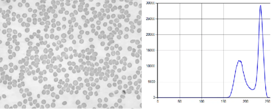
thresholding is a suitable segmentation technique, and several analytic approaches to the threshold calculation have been proposed [139], [140]. For such images, the resulting histogram is bimodal as shown in Figure 6, where one peak is formed by the object's pixels and the other peak is formed by the background pixels. The gray-levels between the two peaks normally result from border pixels between the object and the background. Thus, it makes sense to select a threshold value the gray-level that has a minimum histogram value between the two referred peaks [141]. This technique is called mode method [142].

Figure 6 – Blood cells image and Image Histogram

Imaging aspects as uneven illumination can make a perfectly segmentable histogram into one that cannot be divided by a global threshold because the lighting effect can result in a non-bimodal histogram. In order to enhance the shape of the histogram, to create a better peak-to-valley ratio, is used as a method where that weight the histogram contributions by means of the pixel’s gradient. The pixels gradient can describe if the pixels belong closer to the edge or if it doesn’t. Thus, the pixel gradient can be used to create a histogram where the border pixels are restrained and used only the pixels that belong to the object or the background. This histogram will have the peak-to-valley ratio needed, because all the edge pixels have been suppressed, allowing a simple determination of the threshold value. In a similar thought, the pixel’s gradient can produce a histogram where only the edge pixels, the pixels with the higher gradient, are used, where the object and the background are restrained, and will not be used to build the histogram. This will create a unimodal histogram in witch just the border pixels are present, and where the peak gray level is the selected threshold value.

The utilization of the Laplacian can generate information to whether the pixel belongs on the dark or the light side of an edge. Weszka [139] recommended the utilization of a Laplacian operator intending to improve the histogram to help in the threshold definition. The Laplacian has a value of 0 on a linear ramp formed at the border between object and background but estimates an absolute high value on the edge of the ramp. Using just pixels with high absolute Laplacian values, it creates a bimodal histogram with an unmistakable valley between the peaks. The threshold value can be chosen as the minimum value of the valley between the two peaks. Methods like this are called histogram transformation methods, and there are several approaches in the literature [74], [143]–[149].

Another concern relating image segmentation is when there are various objects in the same image, and these objects touch each other, when the gray-levels of the object can be mistaken with the background gray-gray-levels, when the proportions of the object and the background in the image are very different. Even when the histogram is bi-modal, there can be problems to obtain a correct segmentation if the background has different gray-levels intensities.

One method to deal with such circumstances is adaptive thresholding, which consists in partitioning the image in smaller sub-images and works them independently to reach the threshold value to every sub-image. The principal thought in this sort of approach is to arrange the pixels by comparing its gray values with a value from a set of neighboring gray levels. The region of the neighborhood is called window and its size and shape differ in the different methods. Bernsen’s [150] propose a method that uses adaptive thresholding. In this method, for every pixel (𝑥, 𝑦), the threshold is computed as the arithmetic mean of the highest and the lowest gray levels in a square 𝑟 × 𝑟 neighborhood with the center at the pixel. If the difference between the highest and the lowest gray-levels is lower than a given constant, then the neighborhood consists only of one class and the pixel is categorized as an object or background. This avoids thresholding of very low contrast objects and noise.

Optimal threshold methods are another approach to image thresholding, and these are based on the image histogram by means of a weighted sum of two

or more probability densities with a normal distribution. The threshold value is the gray-level that is closest to the minimum probability between the maxima of two or more normal distributions, creating a minimum error segmentation [61], [151], [152]. The firsts segmentations examples by optimum thresholding were introduced by Chow and Kaneko in 1972 [151] with the purpose for automatically contour the boundaries of the heart ventricles in cardiograms. Likewise, this method represents the use of local histogram and adaptive thresholding. In furtherance to reach the optimal threshold, the image was divided into various 50% non-overlapping sub-images and computed their histogram individually. Each histogram is approximated by a mixture of two Gaussian distributions as part of the bimodality test. In this phase, the thresholds were assigned to the bimodal histograms, and the thresholds of the remaining sub-images were obtained by interpolation. At that point, was executed a second interpolation point by point using neighboring threshold values with the purpose to define a threshold to all the pixels of the image. At last, after using the thresholds values to create the binary image by means, the edges were acquired by taking its gradient.

The estimation of the normal distribution parameters simultaneously with the distribution ambiguity may be considered normal are the main troubles in these methods. However, if the optimal threshold values attempt to maximize the gray-level variance between the objects and the background, these troubles might be overcome. Numerous methods to compute image optimal threshold value have been proposed in the literature [153]–[159]. Among the arrangement of existing methods, we have chosen five of the most prominent and referenced from various categories: The Rosenfeld’s convex hull method [160], Otsu’s clustering method[153], Kittler and Illingworth’s minimum error thresholding [154], Kapur’s entropic method [159] and Abutaleb’s two-dimensional entropy method [161].

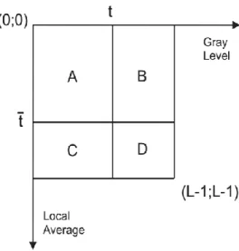
The following notation will be used to briefly explain the referred methods: Let 𝑄 be a 𝑀 × 𝑁 image with 𝐿 gray-levels so that 0 ≤ 𝑞 ≤ 𝐿 − 1. Let ℎ(𝑞) be the image histogram (number of occurrences of the intensity, 𝑞 in the image) and 𝑝(𝑞) the probability mass function (PMF) of the image. The gray level histogram is normalized and regarded as a probability distribution function, defined as:

𝑝(𝑖) = ℎ(𝑖) 𝑀 × 𝑁

The probability density function 𝑝(𝑖) calculates the probability that the intensity value 𝑖 occurs in the image 𝑄.

The cumulative probability function is defined as:

𝑃(𝑖) = ∑ 𝑝(𝑖) 𝑞 𝑖=𝑜

Denoting by 𝑡 the threshold value, the PMFs of the object, 𝑃𝑜(𝑞) for 0 ≤ 𝑞 ≤ 𝑡, and the background, 𝑃𝑏(𝑞) for 𝑡 + 1 ≤ 𝑞 ≤ 𝐿 − 1, are calculated as follows: 𝑃𝑜(𝑡) = 𝑃𝑜= ∑ 𝑝(𝑞) 𝑡 𝑞=0 𝑃𝑏(𝑡) = 𝑃𝑏 = ∑ 𝑝(𝑞) 𝐿−1 𝑞=𝑡+1

The object and background means and variances as functions of the threshold value t are defined as follows:

𝑚𝑜(𝑡) = ∑ 𝑞𝑝(𝑞) 𝑡 𝑞=0 and 𝜎𝑜2(𝑡) = ∑[𝑞 − 𝑚𝑜(𝑡)]2𝑝(𝑞) 𝑡 𝑞=0 𝑚𝑏(𝑡) = ∑ 𝑞𝑝(𝑞) 𝐿−1 𝑞=t+1 and 𝜎𝑏2(𝑡) = ∑ [𝑞 − 𝑚𝑏(𝑡)]2𝑝(𝑞) 𝐿−1 𝑞=𝑡+1

The Rosenfeld’s convex hull method [160] depends on the analysis of the concavity structure of the histogram ℎ(𝑞) characterized by its convex hull 𝐻𝑢𝑙𝑙(𝑞). At the point when the convex hull of the histogram is calculated, the deepest