CERN-EP/2016-054 2016/09/20
CMS-HIG-14-032
Search for Higgs boson off-shell production in
proton-proton collisions at 7 and 8 TeV and derivation of
constraints on its total decay width
The CMS Collaboration
∗Abstract
A search is presented for the Higgs boson off-shell production in gluon fusion and
vector boson fusion processes with the Higgs boson decaying into a W+W−pair and
the W bosons decaying leptonically. The data observed in this analysis are used to constrain the Higgs boson total decay width. The analysis is based on the data col-lected by the CMS experiment at the LHC, corresponding to integrated luminosities
of 4.9 fb−1at a centre-of-mass energy of 7 TeV and 19.4 fb−1at 8 TeV, respectively. An
observed (expected) upper limit on the off-shell Higgs boson event yield normalised to the standard model prediction of 2.4 (6.2) is obtained at the 95% CL for the gluon fusion process and of 19.3 (34.4) for the vector boson fusion process. Observed and expected limits on the total width of 26 and 66 MeV are found, respectively, at the 95% confidence level (CL). These limits are combined with the previous result in the ZZ channel leading to observed and expected 95% CL upper limits on the width of 13 and 26 MeV, respectively.
Published in the Journal of High Energy Physics as doi:10.1007/JHEP09(2016)051.
c
2016 CERN for the benefit of the CMS Collaboration. CC-BY-3.0 license
∗See Appendix A for the list of collaboration members
1
Introduction
A new particle, with properties consistent with those of the standard model (SM) Higgs
bo-son(H), was discovered at the CERN LHC with a mass near 125 GeV by the ATLAS and CMS
collaborations [1–3]. Several properties of this particle have been measured to check its
consis-tency with the SM [4–9]. Direct measurements of the total decay width of the Higgs boson(ΓH)
gave upper limits of 3.4 GeV in the 4`decay channel (where lepton,`, corresponds to either an
electron or a muon) [8] and 2.4 GeV in the γγ decay channel [7, 10], which makes the particle compatible with a single narrow resonance. At the LHC, the precision of direct width measure-ments is limited by the instrumental resolution of the ATLAS and CMS experimeasure-ments, which is three orders of magnitude larger than the expected natural width for the SM Higgs boson, ΓSM
H ∼4.1 MeV [11]. The ratio of the natural width of the discovered boson with respect to that
of the SM Higgs boson was assessed by ATLAS [12] in the combination of all on-shell decay
modes, including invisible and undetectable ones, and found to be ΓH/ΓSMH = 0.64
+0.40 −0.25
un-der the model-dependent assumption that couplings of the 125 GeV boson to W and Z bosons could not be greater than those in the SM. The sizable off-shell production of the Higgs boson can also be used to constrain its natural width. A measurement of the relative off-shell and
on-shell production provides direct information onΓH[13–18], as long as the Higgs boson off- and
on-shell production mechanisms are the same as in the SM and the ratio of couplings governing off- and on-shell production remains unchanged with respect to the SM predictions. For exam-ple, we assume that the dominant production mechanism is gluon fusion (GF) and not quark-antiquark annihilation. Also, we assume that GF production is dominated by the top quark loop and there are no beyond-SM particles significantly contributing in the entire on/off-shell mass range probed by the analysis. Finally, the relative rate of off-shell and on-shell produc-tion depends on the tensor structure of the couplings for the discovered boson [19, 20]. Possible contributions from anomalous couplings are not considered in this analysis.
The CMS experiment already used off-shell production to constrainΓH, using H→ZZ decays
to 4`and 2`2ν final states, and obtained observed (expected) upper limits ofΓH<22(33)MeV
at the 95% confidence level (CL) [21]. The 4`analysis was later updated [22] to include some
improvements and allow for studies of anomalous H → ZZ couplings via their effect on the
off-shell production.
Similarly, ATLAS presented a study in the ZZ and WW channels that constrained the observed (expected) upper limit on the off-shell event yield normalised to the SM prediction (signal
strength µ) to the range of 5.1–8.6 (6.7–11.0). The range is determined by varying the gg→WW
and gg → ZZ background K factor within the uncertainty of the higher-order QCD
correc-tion [23]. An observed (expected) upper 95% CL limit of ΓH < 23(33)MeV was obtained,
assuming the background K factor is equal to the signal K factor.
This paper presents an analysis to constrainΓHand the off-shell signal strength in the leptonic
final states of the H → WW decay, based on the method proposed in Ref. [24]. Our analysis
follows the same methodology as used in the ZZ analysis mentioned above [21]. The WW channel has worse mass resolution than ZZ, which affects the width measurement. However, the WW channel benefits from a significantly larger branching fraction and a lower threshold
for off-shell H→WW production [18]. To maximize sensitivity, the results of this analysis are
combined with those obtained in the H→ZZ channel [21, 22].
The WW and ZZ analyses are based on proton-proton (pp) collision data collected by the CMS
experiment at the LHC in 2011 and 2012, corresponding to integrated luminosities of 4.9 fb−1
2 3 Event datasets and Monte Carlo simulation samples
The paper is organized as follows: after a brief description of the CMS detector in Section 2, event datasets and Monte Carlo (MC) simulation samples are presented in Section 3. The object reconstruction and event selection are described in Sections 4 and 5, respectively. These are followed by the analysis strategy in Section 6 and a description of systematic uncertainties
in Section 7. The individual results for the H → WW channel and the combination of these
results with those from the ZZ channels are reported in Sections 8 and 9, and the summary is given in Section 10.
2
The CMS detector
The central feature of the CMS apparatus is a superconducting solenoid of 6 m internal diam-eter, providing a magnetic field of 3.8 T. Within the solenoid volume there are a silicon pixel and strip tracker, a lead tungstate crystal electromagnetic calorimeter (ECAL), and a brass and scintillator hadron calorimeter, each composed of a barrel and two endcap sections. Forward calorimeters extend the pseudorapidity coverage provided by the barrel and endcap detectors
up to |η| < 5. Muons are measured in gas-ionization detectors embedded in the steel
flux-return yoke outside the solenoid. The missing transverse momentum vector~pTmissis defined as
the projection on the plane perpendicular to the beams of the negative vector sum of the
mo-menta of all reconstructed particles in an event. Its magnitude is referred to as EmissT . A more
detailed description of the CMS detector, together with a definition of the coordinate system and the relevant kinematic variables can be found in [27].
3
Event datasets and Monte Carlo simulation samples
The explicit final state used is the different-flavor dilepton final state W+W− → e±νµ∓ν. The
same-flavor dilepton final states W+W− → e+νe−ν/µ+νµ−ν are not considered, as they are
overwhelmed by background from the Drell–Yan Z/γ∗ → `+`−production.
The events are triggered by requiring the presence of either one or two high-pT electrons or
muons with tight lepton identification and isolation criteria and with|η| <2.4(2.5)for muon
(electron) [28, 29]. Triggers with a single lepton have electron (muon) pT thresholds ranging
from 17 to 27 (24) GeV. The higher thresholds are used for data taking periods with higher
instantaneous luminosity. For the dilepton triggers, one lepton with pT >17 GeV and another
with pT > 8 GeV are required. The average combined trigger efficiency for events that pass
the full event selection is 96% as measured in independent datasets obtained using different triggers.
This analysis uses the dominant SM Higgs boson production modes of GF and vector boson fusion (VBF). Other processes are not expected to contribute significantly to off-shell produc-tion [21]. The analysis accounts for possible interference between the Higgs boson signal and background processes when both have identical initial and final states. Relevant leading order (LO) Feynman diagrams for GF and VBF processes for signal and background, which interfere with the signal, are depicted in Figs. 1 and 2, respectively. Following the previous study in the
ZZ channels [21], a Higgs boson mass of mH = 125.6 GeV [8], with widthΓH =4.15 MeV [11],
is assumed for all of the event generation. The small difference from the combined CMS and
ATLAS Higgs boson mass, 125.1±0.2 GeV [30], is found to have negligible impact on the width
calculation.
The on-shell GF (VBF) signal, tt, and tW processes are generated with thePOWHEG1.0
Figure 1: Feynman diagrams for the GF channel: (left) for the signal process gg → H(H∗) →
W+W−, and (right) for the GF-initiated continuum background process gg → W+W−. The
two processes can interfere, as they have identical initial and final states.
Figure 2: Feynman diagrams for the VBF channel: (left) for the signal process qq →
qqH(H∗) → qqW+W− → qq`+
ν`−ν, and (center and right) for two examples of background
qq→qqW+W−→qq`+
ν`−νchannels.
are simulated using the MADGRAPH 5.1 event generator [36] as described in detail in the
on-shell H→W+W−analysis [37].
For the specific description of the Higgs boson off-shell region, the Higgs boson signal, the
continuum gg→WW background, and their signal-background interference samples are
gen-erated usingGG2VV3.1.5 [38] for GF production, and PHANTOM1.2.5 [39] for VBF production
at LO accuracy with the SM Higgs boson width. The CTEQ6L [40] LO parton distribution
func-tions (PDF) are used byGG2VVand PHANTOM. The dynamic factorization and renormalization
scales of quantum chromodynamics (QCD) forGG2VVare set to half the invariant mass of two
W bosons, µF = µR = mWW/2. For PHANTOM the QCD scale is set to Q2 = M2W+ 16∑
6 i=1p2Ti,
where pTi denotes the transverse momentum of the ith particle in the final state with 6
par-ticles defined in Fig. 2 [39]. The cross sections and various distributions at generator level
obtained fromGG2VVare cross-checked by comparing them toMCFM6.8 [41] results. For all
processes, the parton showering and the hadronization are implemented using PYTHIA
(ver-sion 6.422) [42].
The K factor for the GF process gg→H→ WW is known up to next-to-next-to-leading-order
(NNLO) [43, 44]. A value in the range 1.6–2.6 has been obtained with an approximately flat
de-pendency on mWW. For this analysis we use a value K=2.1 affected by an uncertainty as large
as 25% as discussed in Section 7. A soft collinear approximation for the NNLO QCD calculation of the signal-background interference for the GF processes is reported in [43], which shows that the K factor computed for the SM Higgs boson signal process is a good approximation to the interference process K factor. A similar study using soft gluon resummation confirms the same K factor for the signal and the interference term at next-to-leading order (NLO) and NNLO [44].
The NLO QCD corrections to the LO background GF process, gg→WW, are computed in the
heavy top quark approximation [45], which shows that the K factor for the background is sim-ilar to that for the signal. Therefore, the K factor calculated in the on-shell signal phase space is
4 4 Object reconstruction
also used for the background and the interference term based on theoretical expectations. The K factor, defined as the ratio of NLO to LO cross sections for VBF production, has been shown to be close to unity by the NLO calculation of electroweak and QCD processes, with a 2% theo-retical uncertainty from missing higher-order effects [46]. The QCD NNLO calculations [47, 48] provide an identical cross section as obtained with the QCD NLO calculation within a theoret-ical uncertainty of about 2%. Therefore the K factor of the VBF process is set to unity with a 2% theoretical uncertainty.
In the GG2VV samples, jets are generated by the parton shower algorithm implemented in
PYTHIA. A better jet categorization is obtained with the NLO generatorPOWHEG 1.0. The jet
multiplicity of the GF GG2VV sample is reweighted to take advantage of the jet description
at the matrix element level in POWHEG. A ”jet bin migration scale factor” is estimated as a
function of the generator-level mWWby the comparison of the reconstruction-levelGG2VVmWW
spectrum to thePOWHEGmWWspectrum for each jet bin. As an example, the jet bin migration
scale factor for the 0-jet bin varies by about 20% in the range 160 GeV<mWW<1 TeV, reducing
the number of events in the 0-jet bin in the low-mWW region and increasing this number in
the high-mWW region. This jet bin migration scale factor is applied as a weight to the GG2VV
sample used in this analysis. The scale factor, calculated with the signal sample, is assumed to be the same for the background and interference samples. The application of the factor to the background and interference samples has a negligible effect on the results.
The detector response is simulated using a detailed description of the CMS detector based on
the GEANT4 package [49]. Minimum bias events are merged into the simulated events to
re-produce the additional pp interactions in each bunch crossing (pileup). The simulated samples are reweighted to represent the pileup distribution as measured in the data. The average num-bers of pileup interactions per beam crossing in the 7 TeV and 8 TeV data are about 9 and 21, respectively.
4
Object reconstruction
The particles candidates (e, µ, photon, charged hadron, and neutral hadron) in an event are reconstructed using the particle-flow algorithm [50, 51]. Clusters of energy deposition mea-sured by the calorimeters, and tracks identified in the central tracking system and in the muon detectors, are combined to reconstruct individual particles.
Events used in this analysis are required to have two high-pT lepton candidates (an electron
and a muon) originating from a single primary vertex. Among the vertices identified in an
event, the one with the largest∑ p2T, where the sum runs over all tracks associated with the
vertex, is selected as the primary vertex.
Electron candidates are defined by a reconstructed track in the tracking detector pointing to a cluster of energy deposition in the ECAL [29]. The electron energy is measured primarily from the ECAL cluster energy, including bremsstrahlung recovery in the energy reconstruction by means of the standard CMS ECAL clustering algorithm. A dedicated algorithm combines the momentum of the track and the ECAL cluster energy, improving the energy resolution. A multivariate approach is employed to identify electrons, which combines several measured quantities describing track quality, ECAL cluster shapes, and the compatibility of the measure-ments from the tracker and the ECAL.
A muon candidate is identified by the presence of a track in the muon system matching a track reconstructed in the silicon tracker [28]. The precision of the measured momentum, based on
the curvature of the track in the magnetic field, is ensured by the acceptability criteria of the global fit in the muon system and the hits in the silicon tracker. Photon emission from a muon can affect the event reconstruction, therefore a dedicated algorithm identifies such cases and rejects the corresponding events.
Electrons and muons are required to be isolated to distinguish between prompt leptons from W/Z boson decays and leptons from hadron decays or misidentified leptons in multijet pro-duction. Isolation criteria are based on the scalar sum of the transverse momenta of particles
(scalar pTsum) in the isolation cone defined by∆R=
√
(∆η)2+ (∆φ)2around the leptons. The
scalar pT sum excludes the contribution of the candidate lepton itself. To remove the
contri-bution from the overlapping pileup interactions in this isolation region, the charged particles included in the computation of the isolation variable are required to originate from the primary vertex. The contribution of pileup photons and neutral hadrons is estimated by the average
particle pT density deposited by neutral pileup particles, and is subtracted from the isolation
cone [52]. The relative electron isolation is defined by the ratio of the scalar pT sum in the
isolation cone of ∆R = 0.3 to the transverse momentum of the candidate electron. Isolated
electrons are selected by requiring the relative isolation to be below∼10%. The exact threshold
value depends on the electron η and pT [53, 54]. For each muon candidate, the scalar pT sum
is computed in isolation cones of several radii around the muon direction. This information is combined using a multivariate algorithm that exploits the particles momentum deposition in the isolation annuli to discriminate between prompt muons and the muons from hadron decays inside a jet [28].
Jets are reconstructed using the anti-kT clustering algorithm [55] with a distance parameter
of 0.5, as implemented in the FASTJET package [56, 57]. A correction is applied to account
for the pileup contribution to the jet energy similar to the correction applied for the lepton
isolation. A combinatorial background arises from low-pT jets from pileup interactions which
get clustered into high-pT jets. A multivariate selection is adopted to separate jets from the
primary interaction and those reconstructed due to energy deposits associated with pileup
interactions [58]. Jets considered for the event categorization are required to have pT>30 GeV
and|η| <4.7(4.5)for the 8 (7) TeV analysis.
The identification of bottom(b)quark decays is used to veto the background processes
con-taining top quarks that subsequently decay to a b quark and a W boson. The b quark decay is identified by b quark jet (b jet) tagging criteria based on the impact parameter significance of the constituent tracks or the presence of a soft muon in the event from the semileptonic decay of the b quark [59]. For the former, the track counting high efficiency (TCHE) algorithm [59, 60] is used with a discriminator value greater than 2.1. For the latter, soft muon candidates are
defined without isolation requirements to be within ∆R = 0.4 from a jet and are required to
have pT >3 GeV. These b tagging criteria retain∼95% of the light-quark and gluon jets, while
vetoing∼70% of b jets that arise from events with top quarks.
A projected ETmiss variable is defined as the component of~pTmiss transverse to the nearest
lep-ton if the leplep-ton is situated within the φ window of±π/2 from the~pTmiss direction, otherwise
the projected Emiss
T is the EmissT of the event. A selection using this observable efficiently rejects
Z/γ∗ →τ+τ−background events, in which the~pTmissis preferentially aligned with the leptons,
as well as Z/γ∗ → `+`− events with mismeasured~pmiss
T caused by poorly reconstructed
lep-tons. Since the~pTmiss resolution is degraded by pileup, the minimum of two projected EmissT
variables is used (ET,minmiss ): one constructed from all identified particles (full projected ETmiss), and another one from only the charged particles associated with the primary vertex (track
6 6 Analysis strategy
ETmiss’s from which it is built as shown in Ref. [37].
5
Event selection
Two main production processes are considered, GF and VBF, for which the method to
deter-mineΓHis identical, while event selections differ. To increase the sensitivity to the SM Higgs
boson signal, events with a high-pTlepton pair of different flavor (one electron and one muon,
eµ) are selected, and categorized according to jet multiplicities: zero jets (0-jet category), one jet (1-jet category), and two or more jets (2-jet category). Higgs boson signal events in the 0-and 1-jet categories are mostly produced by the GF process, whereas the 2-jet category is more sensitive to the VBF production.
The WW baseline selection criteria are the same as those used in the on-shell H→WW
analy-sis [37]. For all jet multiplicity categories, candidate events are required to have two oppositely
charged different-flavor leptons with p`1
T >20 GeV for the leading lepton and p
`2
T >10 GeV for
the sub-leading lepton. Lepton pseudorapidities are restricted to be in the acceptance region of
the detector,|η| <2.5(2.4)for electrons (muons). A small number of the electrons and muons
considered in the analysis come from leptonic decays of τ leptons after high pTcuts of lepton.
Using simulation, the signal contribution of τ leptonic decay from the H→WW process, with
one or both W bosons decaying to τν, is estimated to be about 10%. The EmissT,min variable is
required to be above 20 GeV to suppress Z/γ∗ → `+`− and Z/γ∗ →
τ+τ− backgrounds. The
analysis requires the invariant mass of the dilepton m`` > 12 GeV to reject the contributions
from charmonium and bottomonium resonance decays. Events having any b jet are vetoed in order to suppress background events with top quarks. The selection defined above is referred to as the WW baseline selection.
The GF selection consists of the WW baseline selection and is applied to events of the 0-jet and 1-jet categories. The 2-jet category of the WW baseline selection is enriched in VBF production
by requiring that the two highest pT jets are separated by |∆ηjj| > 2.5. In addition the
pseu-dorapidity of each lepton i must obey the relation|ηli − (ηj1+ηj2)/2|/|∆η
jj| <0.5, where ηli,
ηj1 and ηj2 are the pseudorapidities of the lepton and the two jets, and∆η
jj is the η distance
between the two highest pT jets. These cuts are based on the ”VBF cuts” defined in Ref. [61],
exploiting the topology of VBF events. The invariant mass mjj of the two highest pTjets must
be larger than 500 GeV. For events with three or more jets, the lowest pT jets should not be
between the two highest pTjets in η.
6
Analysis strategy
The events retained after the WW baseline selection and the subsequent GF and VBF catego-rization are further partitioned into two sub-samples. The first sub-sample, where events are
required to have m`` < 70 GeV is attributed to the on-shell Higgs boson category, while the
second sub-sample with m`` > 70 GeV is attributed to the off-shell Higgs boson category. The
expected on-shell Higgs boson signal is 196 (3) events in the on(off)-shell category and the ex-pected off-shell Higgs boson signal is 2 (7) events in the on(off)-shell category for 0-jet events after the baseline selection. The level of on- and off-shell Higgs boson separation is shown in Figs. 4 and 5 where the left (right) column shows the distributions in the on(off)-shell category.
The selection criteria for the on-shell category is the same as the previous on-shell H→W+W−
study [37], but is modified for the off-shell region as p``T > 45 GeV and pT`2 > 20 GeV due to
is defined as mHT = √
2p``TETmiss(1−cos∆φ(~p``T,~pTmiss)), where~p``T is the dilepton transverse
momentum vector, p``T is its magnitude, and∆φ(~p``T,~pTmiss)is the azimuthal angle between the
dilepton momentum and~pTmiss. The mHT and the m``are used to discriminate the Higgs boson
signal from the dominant WW and top quark pair, W+jets, and W+γ(∗)backgrounds.
In order to enhance the sensitivity, a boosted decision tree [62] multivariate discriminator
(MVA) is implemented with the toolkit for multivariate analysis (TMVA) package [63] and
is trained to discriminate between the off-shell Higgs boson signal and the other SM
back-grounds. Seven variables, mHT, m``, the opening angle∆φ``between the two leptons, p``T, EmissT
in an event, pT`1, and pT`2, are used for the boosted decision tree training and enter into the
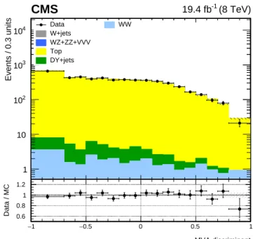
MVA discriminant. Figure 3 shows the MVA discriminant distribution tested on a top quark
enriched region with 1 b-tagged jet of pT > 30 GeV, where good agreement between data and
MC simulation is observed. After validation of the MVA discriminant variable with 8 TeV MC
MVA discriminant 1 − −0.5 0 0.5 1 Events / 0.3 units 1 10 2 10 3 10 4 10 Data W+jets WZ+ZZ+VVV Top DY+jets WW CMS 19.4 fb-1 (8 TeV) MVA discriminant 1 − −0.5 0 0.5 1 Data / MC 0.6 0.8 1 1.2
Figure 3: The MVA discriminant distribution for 8 TeV data for the 1-jet category in the top
quark control region with one b-tagged jet of pT >30 GeV. The Z, W+jets, WW, and top quark
simulation predictions are corrected with the estimates based on control samples in data, while other contributions are taken from simulation.
simulation and data for the 0- and 1-jet categories, the discrimination in these categories is
per-formed using the m`` and MVA variables, which achieve a 4% improvement on the expected
width limit compared to the m``and mHT variables. The analysis of other categories (8 TeV 2-jet
category and all three of 7 TeV dataset categories) use the m``and mHT variables. The selections
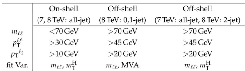
and fit variables for the on and off-shell regions are given in Table 1.
Twelve two-dimensional (2D) distributions m`` versus mHT (m`` versus MVA for 8 TeV 0, 1-jet
categories) with variable bin size are defined. The bin widths are optimized to achieve good separation between the SM Higgs boson signal and backgrounds, while maintaining adequate statistical uncertainties in all the bins. A 2D binned likelihood fit is performed simultaneously to these twelve distributions using template 2D distributions which are obtained from the sig-nal and background simulation. For both the GF and VBF cases, expected event rates per bin
are constructed to be on-, or off-shell SM Higgs boson signal-like(PH), background-like(Pbkg)
8 6 Analysis strategy
Table 1: Analysis region definitions for on- and off-shell selections.
On-shell Off-shell Off-shell
(7, 8 TeV: all-jet) (8 TeV: 0,1-jet) (7 TeV: all-jet, 8 TeV: 2-jet)
m`` <70 GeV >70 GeV >70 GeV
pT`` >30 GeV >45 GeV >45 GeV
pT`2 >10 GeV >20 GeV >20 GeV
fit Var. m``, mHT m``, MVA m``, mHT
likelihood function depending on the SM Higgs boson GF (VBF) signal strength in the off-shell region µoff-shellGF (µoff-shellVBF ) without correlation to the on-shell GF (VBF) signal strength µGF
(µVBF), the total expected event rates per bin (Ptot(m``, mHT(MVA)|µs)) can be written using
these functions following [17, 64] as
Ptot(m``, mHT(MVA)|µs) =µoff-shellGF P gg H, off-shell+ q µoff-shellGF Pintgg+ Pbkggg +µoff-shellVBF PH, off-shellVBF + q µoff-shellVBF PintVBF+ PbkgVBF + µGFPH, on-shellgg +µVBFPH, on-shellVBF + P qq bkg+ Pother bkg. (1)
Here,Pbkgqq is the contribution from the qq → WW continuum background, andPother bkg
in-cludes the other background contributions. Similarly, the likelihood function of the total width ΓHis obtained with the total expected event rates per bin(Ptot(m``, mHT(MVA)|r))
Ptot(m``, mHT(MVA)|r) =µGFrPH, off-shellgg +
√ µGFrPintgg+ P gg bkg + µVBFrPH, off-shellVBF + √ µVBFrPintVBF+ PbkgVBF + µGFPH, on-shellgg +µVBFPH, on-shellVBF + P qq bkg+ Pother bkg, (2) where, r = ΓH/ΓSM
H is the scale factor with respect to theΓSMH determined by the Higgs boson
mass value used in the simulation.
The normalisation and shape of the template 2D distributions used in the fit for the background processes are obtained following the same procedure as in Ref. [37]. Most of the background
processes such as top quark, Wγ∗, and W+jets production, are estimated from data control
regions. The normalisation of the qq→WW background is constrained by the fit of m``versus
mH
T or m``versus MVA discriminant distribution using shapes determined by simulation. For
the 2-jet category, the WW background normalization is taken from the MC simulation. After
the template fit to the m``versus mHT (MVA) distributions for µs andΓH, the observed projected
mHT (MVA) distributions are compared to the fit results in Figs. 4 and 5. In these figures, each
process is normalized to the result of the 2D template fit and weighted using the other variable
m``. This means that for the mHT (MVA) distributions, the m``distribution is used to compute
the ratio of the fitted signal (S) to the sum of signal and background (S+B) in each bin of the m``
distribution integrated over the mHT (MVA) variable. In Fig. 4, the observed mHT distributions
are shown for the GF mode 0- and 1-jet categories and for the VBF mode 2-jet category for 7 TeV
data. The mH
T or MVA discriminant distributions of 8 TeV data are presented for the GF mode
[GeV]
H T
m
0 100 200 300 400
S/(S+B) weighted events / bin
20 40 Data SM Γ SM off-shell 30 x On-shell (*) γ V W+jets WZ+ZZ+VVV Top DY+jets ggWW WW Bkg uncertainty = 125.6 GeV H m 0-jet µ e CMS -1 (7 TeV) 4.9 fb [GeV] H T m 0 100 200 300 400 Data / MC 0 0.5 1 1.5
(a) GF 0-jet on-shell
[GeV]
H T
m
0 100 200 300 400
S/(S+B) weighted events / bin 10 20 30 40 Data SM Γ SM off-shell 30 x On-shell (*) γ V W+jets WZ+ZZ+VVV Top DY+jets ggWW WW Bkg uncertainty = 125.6 GeV H m 0-jet µ e CMS -1 (7 TeV) 4.9 fb [GeV] H T m 0 100 200 300 400 Data / MC 0 0.5 1 1.5 (b) GF 0-jet off-shell [GeV] H T m 0 100 200 300 400
S/(S+B) weighted events / bin 2
4 6 8 Data SM Γ SM off-shell 30 x On-shell (*) γ V W+jets WZ+ZZ+VVV Top DY+jets ggWW WW Bkg uncertainty = 125.6 GeV H m 1-jet µ e CMS -1 (7 TeV) 4.9 fb [GeV] H T m 0 100 200 300 400 Data / MC 0 0.5 1 1.5 (c) GF 1-jet on-shell [GeV] H T m 0 100 200 300 400
S/(S+B) weighted events / bin
5 10 15 Data SM Γ SM off-shell 30 x On-shell (*) γ V W+jets WZ+ZZ+VVV Top DY+jets ggWW WW Bkg uncertainty = 125.6 GeV H m 1-jet µ e CMS -1 (7 TeV) 4.9 fb [GeV] H T m 0 100 200 300 400 Data / MC 0 0.5 1 1.5 (d) GF 1-jet off-shell [GeV] H T m 0 100 200 300 400
S/(S+B) weighted events / bin
0.5 1 1.5 Data SM Γ SM off-shell 30 x On-shell (*) γ V W+jets WZ+ZZ+VVV Top DY+jets ggWW WW Bkg uncertainty = 125.6 GeV H m 2-jet µ e CMS 4.9 fb-1 (7 TeV) [GeV] H T m 0 100 200 300 400 Data / MC 0 0.5 1 1.5
(e) VBF 2-jet on-shell
[GeV]
H T
m
0 100 200 300 400
S/(S+B) weighted events / bin
1 2 3 Data SM Γ SM off-shell 30 x On-shell (*) γ V W+jets WZ+ZZ+VVV Top DY+jets ggWW WW Bkg uncertainty = 125.6 GeV H m 2-jet µ e CMS 4.9 fb-1 (7 TeV) [GeV] H T m 0 100 200 300 400 Data / MC 0 0.5 1 1.5 (f) VBF 2-jet off-shell
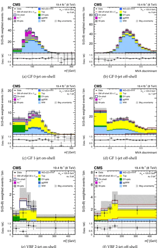
Figure 4: The mHT distributions for the GF 0-jet (a) and (b), and 1-jet (c) and (d) categories, and
the VBF 2-jet category (e) and (f) for 7 TeV data. The distributions are weighted as described in the text. In the histogram panels, the expected off-shell SM Higgs boson signal rate, including
signal-background interference, is calculated forΓH = 30ΓSMH and is shown with and without
stacking on top of the backgrounds. In the data/MC panels, the expected off-shell SM Higgs
10 6 Analysis strategy [GeV] H T m 0 100 200 300
S/(S+B) weighted events / bin 20
40 60 80 Data SM Γ SM off-shell 30 x On-shell (*) γ V W+jets WZ+ZZ+VVV Top DY+jets ggWW WW Bkg uncertainty = 125.6 GeV H m 0-jet µ e CMS -1 (8 TeV) 19.4 fb [GeV] H T m 0 100 200 300 Data / MC 0 0.5 1 1.5
(a) GF 0-jet on-shell
MVA discriminant
1
− −0.5 0 0.5 1
S/(S+B) weighted events / bin 20 40 60 80 Data SM Γ SM off-shell 30 x On-shell (*) γ V W+jets WZ+ZZ+VVV Top DY+jets ggWW WW Bkg uncertainty = 125.6 GeV H m 0-jet µ e CMS -1 (8 TeV) 19.4 fb MVA discriminant 1 − −0.5 0 0.5 1 Data / MC 0 0.5 1 1.5 (b) GF 0-jet off-shell [GeV] H T m 0 100 200 300
S/(S+B) weighted events / bin 5
10 15 20 Data SM Γ SM off-shell 30 x On-shell (*) γ V W+jets WZ+ZZ+VVV Top DY+jets ggWW WW Bkg uncertainty = 125.6 GeV H m 1-jet µ e CMS -1 (8 TeV) 19.4 fb [GeV] H T m 0 100 200 300 Data / MC 0 0.5 1 1.5 (c) GF 1-jet on-shell MVA discriminant 1 − −0.5 0 0.5 1
S/(S+B) weighted events / bin
20 40 Data SM Γ SM off-shell 30 x On-shell (*) γ V W+jets WZ+ZZ+VVV Top DY+jets ggWW WW Bkg uncertainty = 125.6 GeV H m 1-jet µ e CMS -1 (8 TeV) 19.4 fb MVA discriminant 1 − −0.5 0 0.5 1 Data / MC 0 0.5 1 1.5 (d) GF 1-jet off-shell [GeV] H T m 0 100 200 300 400
S/(S+B) weighted events / bin 1
2 3 Data SM Γ SM off-shell 30 x On-shell (*) γ V W+jets WZ+ZZ+VVV Top DY+jets ggWW WW Bkg uncertainty = 125.6 GeV H m 2-jet µ e CMS 19.4 fb-1 (8 TeV) [GeV] H T m 0 100 200 300 400 Data / MC 0 0.5 1 1.5
(e) VBF 2-jet on-shell
[GeV]
H T
m
0 100 200 300 400
S/(S+B) weighted events / bin 2
4 6 8 Data SM Γ SM off-shell 30 x On-shell (*) γ V W+jets WZ+ZZ+VVV Top DY+jets ggWW WW Bkg uncertainty = 125.6 GeV H m 2-jet µ e CMS 19.4 fb-1 (8 TeV) [GeV] H T m 0 100 200 300 400 Data / MC 0 0.5 1 1.5 (f) VBF 2-jet off-shell
Figure 5: The mHT and MVA discriminant distributions for the GF 0-jet (a) and (b), and 1-jet (c)
and (d) categories, and mH
T for the VBF 2-jet category (e) and (f) for 8 TeV data. More details are
7
Systematic uncertainties
The systematic uncertainties for this analysis, presented in Table 2, are classified into three cat-egories as described in detail in Ref. [37] and include uncertainties in the background yield predictions derived from data, experimental uncertainties affecting normalisation and shapes of signal and backgrounds distributions obtained from simulation, and theoretical uncertain-ties affecting signal and background yields estimated using simulation.
The dominant background for the 0-jet category is continuum qq → WW production. The
normalization of the qq → WW background for the 0 (1)-jet categories is determined from
the 2D binned template fit to the data with 8 (18)% uncertainty dominated by the statistical uncertainty in the number of observed events. The template 2D distribution obtained from the
default generator is replaced by another one from POWHEGto estimate the shape uncertainty
in the fit.
Top quark production is the main background for the 1-jet and 2-jet categories. Backgrounds from top quarks are identified and rejected via b jet tagging based on the TCHE and the soft muon tagging algorithms. The efficiency to identify top quark events is measured in a control sample dominated by tt and tW events, which is selected by requiring one b-tagged jet. The total uncertainty in the top quark background contribution is about 10% for 0,1-jet and about 30% for 2-jet category. The scale of these uncertainties is defined by the control sample size (number of events) and the uncertainty of tagging algorithms.
The Z/γ∗ →τ+τ−background process is estimated using Z/γ∗ →µµevents selected in data,
in which muons are replaced with simulated τ decays. The uncertainty in the estimation of this background process is about 10%.
The non-prompt lepton background contributions originating from the leptonic decays of heavy quarks and τ leptons, hadrons misidentified as leptons, and electrons from photon conversions
in W+jets and QCD multijet production, are suppressed by the identification and isolation
re-quirements on electrons and muons, as described in Section 4. The remaining contribution
from the non-prompt lepton background is estimated directly from data. The efficiency, epass,
for a jet that satisfies the loose lepton requirements to pass the standard selection is determined using an independent sample dominated by events with non-prompt leptons from QCD mul-tijet processes. This efficiency is then used to weight the data with the loose selection to obtain the estimated contribution from the non-prompt lepton background in the signal region. The
systematic uncertainty has two sources: the dependence of epass on the sample composition,
and the method. The total uncertainty in epass, including the statistical precision of the control
sample is about 40% for all cases (on- and off-shell, and all jet categories).
The contribution from W/γ∗ background processes is evaluated using a simulated sample, in
which one lepton escapes detection. The K factor of the simulated sample is calculated by data
control regions, where a high-purity control sample of W/γ∗ events with three reconstructed
lepton is defined and compared to the simulation. A factor of 1.5±0.5 with respect to the LO
prediction is found. The shape of the discriminant variables used in the signal extraction for the Wγ process is obtained from data control region that has 200 times more events than the simulated sample [37]. The normalization is taken from simulated samples with uncertainty of 20% dominated by the size of sample.
The integrated luminosity is measured using data from the HF system and the pixel detec-tor [25, 26]. The uncertainties in the integrated luminosity measurement are 2.2% at 7 TeV and 2.6% at 8 TeV.
12 7 Systematic uncertainties
The lepton reconstruction efficiency in MC simulation is corrected to match data using a control
sample of Z/γ∗ → `+`−events in the Z boson peak region [29]. The associated uncertainty is
about 4% for electrons and 3% for muons. The associated shape uncertainty is found to be negligible.
Table 2: Summary of systematic uncertainties. Backgrounds estimated from data
Source Uncertainty qq→WW 8–18% (0,1-jet) tt, tW ∼10% (0,1-jet);∼30% (2-jet) Z/γ∗→τ+τ− ∼10% W+jet, QCD multijet ∼40% Wγ/γ∗ 20–30% Experimental uncertainties Source Uncertainty
Integrated luminosity 2.2% at 7 TeV 2.5% at 8 TeV
Lepton reconstruction and identification 3–4%
Jet energy scale 10%
Theoretical uncertainties Source Uncertainty qq→WW 20% (2-jet) WZ, ZZ, VVV ∼4% QCD scale uncertainties: On-shell signal 20% (GF); 2% (VBF) Off-shell signal 25% (GF); 2% (VBF)
Bkg. and sig. + bkg. interf. 35% (GF); 2% (VBF)
Exclusive jet bin fractions 30–50% (GF); 3–11% (VBF)
PDFs 3–8%
Underlying event and parton shower 20% (GF); 10% (VBF)
Uncertainties in the jet energy scales affect the jet multiplicity and the jet kinematic variables. The corresponding systematic uncertainties are computed by repeating the analysis with varied jet energy scales up and down by one standard deviation around their nominal values [65]. As a result, the uncertainty on the event selection efficiency is about 10%.
For the 2-jet category, the qq→WW background rate is estimated from simulation with a
the-oretical uncertainty of 20% by comparing two different generatorsPOWHEGand MADGRAPH.
The total theoretical uncertainties in the diboson and multiboson production WZ, ZZ, VVV,
(V = W/Z), are estimated from the scale variation of renormalization and factorisation by a
factor of two and are about 4% [66].
The production cross sections and their uncertainties used for the SM Higgs boson expectation are taken from Refs. [67, 68]. The uncertainties in the inclusive yields from missing higher-order corrections are evaluated by the change in the QCD factorization and renormalization scales and propagated to the K factor uncertainty. The K factor uncertainty for the on-shell (off-shell) GF component is as large as 20 (25)% and it is 2% for the VBF production in both
on-and off-shell regions. The gg→WW background and interference K factors for GF production
in the off-shell region are assumed to be the same as the signal K factor with an additional 10% uncertainty [43, 44].
The uncertainty on the predicted yield per jet bin associated with unknown higher order QCD corrections for GF are computed following the Stewart–Tackmann procedure [69]. Samples
have been produced with theSHERPA 2.1.1 generator [70–72], which includes a jet at the QCD
matrix element calculation for gg → WW. The factorization and renormalization scales are
varied by factors of 1/2 and 2. In the off-shell GF production, the uncertainty on the yield in each jet bin is about 30% for the 0- and 1-jet cases and 50% for the 2-jet case. The effect of the large uncertainty in the 2-jet bin is negligible in the final results.
A similar comparison for the shell region is performed for the VBF process, where the
off-shell generation is provided by PHANTOM, which has LO accuracy. Since two jets are generated
at the matrix element level, the correction factor to take into account jet bin migration is small and the uncertainty associated with it varies between 3% and 11%, depending on the jet bin. The impact of variations in the choice of PDFs and QCD coupling constant on the yields
is evaluated following the PDF4LHC prescription [73], using the CT10, NNPDF2.1 [74], and
MSTW2008 [75] PDF sets. For the gluon-initiated signal processes (GF and ttH), the PDF un-certainty is about 8%, while for the quark-initiated processes (VBF and Higgs boson production in association with a vector boson, VH) it is 3–5%.
The systematic uncertainties due to the underlying event and parton shower model [76, 77] are estimated by comparing samples simulated with different parton shower tunes and by disabling the underlying event simulation. The uncertainties are around 20% for GF and 10% for VBF.
The overall sensitivity of the analysis to systematic uncertainties can be quantified as the
rela-tive difference in the observed limits onΓHwith and without systematic uncertainties included
in the analysis; it is found to be about 30%.
8
Constraints on Higgs boson width with WW decay mode
Three separate likelihood scans are performed for the data observed in the twelve 2D distribu-tions described in Section 6:−2∆ lnL(data|µoff-shellGF ),−2∆ lnL(data|µoff-shellVBF ), and−2∆ lnL(data|ΓH),
using data density functions defined by Eqs. (1) and (2), where−2∆ lnLis defined as
−2∆ lnL(data|x) = −2 lnL(data|x)
Lmax . (3)
The profile likelihood function defined in Eq. (3) is assumed to follow a χ2distribution
(asymp-totic approximation [78]). We set 95% CL limits on value x from−2∆ lnL(data|x) =3.84.
When the negative log-likelihood, −2∆ lnL, of µoff-shell
GF (µoff-shellVBF ) is scanned, the other signal
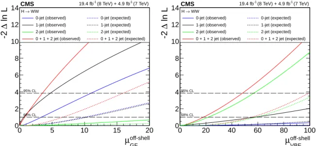
strengths are treated as nuisance parameters. The uncertainties described in Section 7 are in-corporated as nuisance parameters in the scan. The observed (expected) constraints of the off-shell signal strengths for six off-shell 2D distributions (0-jet, 1-jet, 2-jet categories for 7 and 8 TeV data) are µoff-shellGF < 3.5(16.0)and µoff-shellVBF < 48.1(99.2)at 95% CL, as shown in Fig. 6. The tighter than expected constraints arise from the deficit in the observed number of events that is seen consistently in all jet categories in the phase space most sensitive to the off-shell production, as shown in Fig. 5.
The results are shown in Fig. 7 for scans of the likelihood as a function ofΓH. The µGFand µVBF
are treated as nuisance parameters in the likelihood scan ofΓH. The scan combining the 0-, 1-,
and 2-jet categories leads to an observed (expected) upper limit of 26 (66) MeV at 95% CL on
14 9 Constraints on Higgs width with WW and ZZ decay modes off-shell GF µ 0 5 10 15 20 ln L ∆ -2 0 2 4 6 8 10 12 14 WW → H
0-jet (observed) 0-jet (expected) 1-jet (observed) 1-jet (expected) 2-jet (observed) 2-jet (expected) 0 + 1 + 2 jet (observed) 0 + 1 + 2 jet (expected) CMS 19.4 fb-1 (8 TeV) + 4.9 fb-1 (7 TeV) 68% CL 95% CL off-shell VBF µ 0 20 40 60 80 100 ln L ∆ -2 0 2 4 6 8 10 12 14 WW → H
0-jet (observed) 0-jet (expected) 1-jet (observed) 1-jet (expected) 2-jet (observed) 2-jet (expected) 0 + 1 + 2 jet (observed) 0 + 1 + 2 jet (expected) CMS 19.4 fb-1 (8 TeV) + 4.9 fb-1 (7 TeV)
68% CL 95% CL
Figure 6: Scan of the negative log-likelihood as a function of the off-shell GF SM Higgs boson signal strength µoff-shellGF (left) and of the off-shell VBF signal strength µoff-shellVBF (right) for 0-, 1-,
2-jet categories separately and all categories combined for the H→WW process: the observed
(expected) scan is represented by the solid (dashed) line.
pure background hypothesis (µGF = 0, µVBF = 0): once the best-fit µGFand µVBFvalues reach
zero, the likelihood given by Eq. 2 does not depend on r anymore.
The coverage probability of the 95% CL limit has been verified with toy MC simulation samples generated according to different r hypotheses in Eq. (2). The toy MC sample generated with
r =1 has been used to estimate the p-value of an observed limit of<26 MeV, while the expected
one is<66 MeV. A p-value of 3.6% is obtained.
9
Constraints on Higgs width with WW and ZZ decay modes
To exploit the full power of the Higgs boson width measurement technique based on the
off-shell Higgs boson production approach, the results using H → WW reported here are
com-bined with those found using H → ZZ [21, 22]. The H → ZZ results are obtained using
datasets corresponding to an integrated luminosity of 5.1 (19.7) fb−1at 7 (8) TeV. The statistical
methodology used in this combination is the same as the one employed in Ref. [21].
The likelihood of the off-shell signal strength is scanned with the assumption of SU(2) custodial
symmetry for the combination: µZZ
GF/µWWGF = µZZVBF/µWWVBF = ΛWZ = 1. The observed (expected)
constraints on the off-shell signal strengths at 95% CL are µoff-shell
GF < 2.4(6.2)and µoff-shellVBF <
19.3(34.4), as shown in Fig. 8.
For the likelihood scan ofΓH, this analysis considers the possible difference of signal strength
measurements between the two Higgs boson decay modes with an assumption that the ratio
of signal strengths is the same for each GF and VBF processes. Accordingly, µWWGF , µWWVBF, µZZGF,
and µZZVBFcan be expressed in terms of three independent parameters left floating in the fit: µGF,
µVBF, andΛWZ: µWWGF = µGF, µWWVBF = µVBF, µGFZZ=ΛWZµGF, and µZZVBF=ΛWZ·µVBF, where µGFand
µVBFare the Higgs boson signal strengths for the GF and VBF production as in Eq. (2) andΛWZ
is the common ratio µZZGF/µWWGF =µZZVBF/µWWVBF =ΛWZ. Figure 9 shows the combined likelihood
scan as a function of the Higgs boson width. The observed (expected) combined limit for the width corresponds to 13 (26) MeV at 95% CL. The observed limit improves by 50% the result of
(MeV)
HΓ
0
20
40
60
80
ln L
∆
-2
0
2
4
6
8
10
12
14
H → WW0-jet (observed) 0-jet (expected)
1-jet (observed) 1-jet (expected)
2-jet (observed) 2-jet (expected)
0 + 1 + 2 jet (observed) 0 + 1 + 2 jet (expected)
CMS
19.4 fb-1 (8 TeV) + 4.9 fb-1 (7 TeV)68% CL 95% CL
Figure 7: Scan of the negative log-likelihood as a function of ΓH for 0-, 1-, 2-jet categories
separately and all categories combined for the H→WW process: the observed (expected) scan
is represented by the solid (dashed) line.
the H→ WW channel alone (<26 MeV) and by 41% the observed limit of< 22 MeV set in the
H→ZZ channel alone [21]. The result is about a factor of 3 larger than the SM expectation of
ΓH≈4 MeV. Using pseudo data generated with the SM Higgs boson width, the p-value for the
observed limit is 7.4%. The relaxation of the same GF and VBF signal strength ZZ/WW ratios
increases the observed combined 95% CL limit on the width toΓH <15 MeV.
10
Summary
A search is presented for the Higgs boson off-shell production in gluon fusion and vector boson
fusion processes with the Higgs boson decaying into a W+W−pair and the W bosons decaying
leptonically. The data observed in this analysis are used to constrain the Higgs boson total decay width. The analysis is based on pp collision data collected by the CMS experiment at
√
s = 7 and 8 TeV, corresponding to integrated luminosities of 4.9 and 19.4 fb−1 respectively.
The observed and expected upper limits for the off-shell signal strengths at 95% CL are 3.5 and 16.0 for the gluon fusion process, and 48.1 and 99.2 for the vector boson fusion process. The
observed and expected constraints on the Higgs boson total width are, respectively, ΓH < 26
and<66 MeV, obtained at the 95% CL. These results are combined with those obtained earlier
in the H→ZZ channel, which further improves the observed and expected upper limits of the
off-shell signal strengths to 2.4 and 6.2 for the gluon fusion process, and 19.3 and 34.4 for the vector boson fusion process. The observed and expected constraints on the Higgs boson total
16 10 Summary off-shell GF µ 0 5 10 15 20 ln L ∆ -2 0 2 4 6 8 10 12 14 WW (observed) → H H → WW (expected) ZZ (observed) → H H → ZZ (expected) ZZ+WW (observed) → H H → ZZ+WW (expected) CMS 19.7 fb-1 (8 TeV) + 5.1 fb-1 (7 TeV) 68% CL 95% CL off-shell VBF µ 0 20 40 60 80 ln L ∆ -2 0 2 4 6 8 10 12 14 WW (observed) → H H → WW (expected) ZZ (observed) → H H → ZZ (expected) ZZ+WW (observed) → H H → ZZ+WW (expected) CMS 19.7 fb-1 (8 TeV) + 5.1 fb-1 (7 TeV) 68% CL 95% CL
Figure 8: Scan of the negative log-likelihood as a function of off-shell SM Higgs boson signal strength for GF µoff-shell
GF (left) and for VBF µoff-shellVBF (right) from the combined fit of H → WW
and H → ZZ channels for 7 and 8 TeV. In the likelihood scan of µoff-shellGF and µoff-shellVBF , this
analysis assumes the SU(2) custodial symmetry: µZZGF/µWWGF =µZZVBF/µWWVBF =1.
(MeV)
HΓ
0
20
40
60
ln L
∆
-2
0
2
4
6
8
10
12
14
WW (observed) → H H → WW (expected) ZZ (observed) → H H → ZZ (expected) ZZ+WW (observed) → H H → ZZ+WW (expected)CMS
19.7 fb-1 (8 TeV) + 5.1 fb-1 (7 TeV) 68% CL 95% CLFigure 9: Scan of the negative log-likelihood as a function ofΓHfrom the combined fit of H→
WW and H→ZZ channels for 7 and 8 TeV. In the likelihood scan ofΓH, this analysis assumes
the same GF and VBF ratio of signal strengths for WW and ZZ decay modes : µZZGF/µWWGF =
Acknowledgments
We congratulate our colleagues in the CERN accelerator departments for the excellent perfor-mance of the LHC and thank the technical and administrative staffs at CERN and at other CMS institutes for their contributions to the success of the CMS effort. In addition, we grate-fully acknowledge the computing centres and personnel of the Worldwide LHC Computing Grid for delivering so effectively the computing infrastructure essential to our analyses. Fi-nally, we acknowledge the enduring support for the construction and operation of the LHC and the CMS detector provided by the following funding agencies: the Austrian Federal Min-istry of Science, Research and Economy and the Austrian Science Fund; the Belgian Fonds de la Recherche Scientifique, and Fonds voor Wetenschappelijk Onderzoek; the Brazilian Fund-ing Agencies (CNPq, CAPES, FAPERJ, and FAPESP); the Bulgarian Ministry of Education and Science; CERN; the Chinese Academy of Sciences, Ministry of Science and Technology, and Na-tional Natural Science Foundation of China; the Colombian Funding Agency (COLCIENCIAS); the Croatian Ministry of Science, Education and Sport, and the Croatian Science Foundation; the Research Promotion Foundation, Cyprus; the Ministry of Education and Research, Esto-nian Research Council via IUT23-4 and IUT23-6 and European Regional Development Fund, Estonia; the Academy of Finland, Finnish Ministry of Education and Culture, and Helsinki Institute of Physics; the Institut National de Physique Nucl´eaire et de Physique des Partic-ules / CNRS, and Commissariat `a l’ ´Energie Atomique et aux ´Energies Alternatives / CEA, France; the Bundesministerium f ¨ur Bildung und Forschung, Deutsche Forschungsgemeinschaft, and Helmholtz-Gemeinschaft Deutscher Forschungszentren, Germany; the General Secretariat for Research and Technology, Greece; the National Scientific Research Foundation, and Na-tional Innovation Office, Hungary; the Department of Atomic Energy and the Department of Science and Technology, India; the Institute for Studies in Theoretical Physics and Mathematics, Iran; the Science Foundation, Ireland; the Istituto Nazionale di Fisica Nucleare, Italy; the Min-istry of Science, ICT and Future Planning, and National Research Foundation (NRF), Repub-lic of Korea; the Lithuanian Academy of Sciences; the Ministry of Education, and University of Malaya (Malaysia); the Mexican Funding Agencies (BUAP, CINVESTAV, CONACYT, LNS, SEP, and UASLP-FAI); the Ministry of Business, Innovation and Employment, New Zealand; the Pakistan Atomic Energy Commission; the Ministry of Science and Higher Education and the National Science Centre, Poland; the Fundac¸˜ao para a Ciˆencia e a Tecnologia, Portugal; JINR, Dubna; the Ministry of Education and Science of the Russian Federation, the Federal Agency of Atomic Energy of the Russian Federation, Russian Academy of Sciences, and the Russian Foundation for Basic Research; the Ministry of Education, Science and Technologi-cal Development of Serbia; the Secretar´ıa de Estado de Investigaci ´on, Desarrollo e Innovaci ´on and Programa Consolider-Ingenio 2010, Spain; the Swiss Funding Agencies (ETH Board, ETH Zurich, PSI, SNF, UniZH, Canton Zurich, and SER); the Ministry of Science and Technology, Taipei; the Thailand Center of Excellence in Physics, the Institute for the Promotion of Teach-ing Science and Technology of Thailand, Special Task Force for ActivatTeach-ing Research and the National Science and Technology Development Agency of Thailand; the Scientific and Techni-cal Research Council of Turkey, and Turkish Atomic Energy Authority; the National Academy of Sciences of Ukraine, and State Fund for Fundamental Researches, Ukraine; the Science and Technology Facilities Council, UK; the US Department of Energy, and the US National Science Foundation.
Individuals have received support from the Marie-Curie programme and the European Re-search Council and EPLANET (European Union); the Leventis Foundation; the A. P. Sloan Foundation; the Alexander von Humboldt Foundation; the Belgian Federal Science Policy Of-fice; the Fonds pour la Formation `a la Recherche dans l’Industrie et dans l’Agriculture
(FRIA-18 10 Summary
Belgium); the Agentschap voor Innovatie door Wetenschap en Technologie (IWT-Belgium); the Ministry of Education, Youth and Sports (MEYS) of the Czech Republic; the Council of Science and Industrial Research, India; the HOMING PLUS programme of the Foundation for Polish Science, cofinanced from European Union, Regional Development Fund; the Mobility Plus pro-gramme of the Ministry of Science and Higher Education (Poland); the OPUS propro-gramme of the National Science Center (Poland); MIUR project 20108T4XTM (Italy); the Thalis and Aris-teia programmes cofinanced by EU-ESF and the Greek NSRF; the National Priorities Research Program by Qatar National Research Fund; the Programa Clar´ın-COFUND del Principado de Asturias; the Rachadapisek Sompot Fund for Postdoctoral Fellowship, Chulalongkorn Uni-versity (Thailand); the Chulalongkorn Academic into Its 2nd Century Project Advancement Project (Thailand); and the Welch Foundation, contract C-1845.
References
[1] ATLAS Collaboration, “Observation of a new particle in the search for the Standard Model Higgs boson with the ATLAS detector at the LHC”, Phys. Lett. B 716 (2012) 1,
doi:10.1016/j.physletb.2012.08.020, arXiv:1207.7214.
[2] CMS Collaboration, “Observation of a new boson at a mass of 125 GeV with the CMS experiment at the LHC”, Phys. Lett. B 716 (2012) 30,
doi:10.1016/j.physletb.2012.08.021, arXiv:1207.7235.
[3] CMS Collaboration, “Observation of a new boson with mass near 125 GeV in
pp collisions at√s =7 and 8 TeV”, JHEP 06 (2013) 081,
doi:10.1007/JHEP06(2013)081, arXiv:1303.4571.
[4] CMS Collaboration, “Study of the Mass and Spin-Parity of the Higgs Boson Candidate via its Decays to Z Boson Pairs”, Phys. Rev. Lett. 110 (2013) 081803,
doi:10.1103/PhysRevLett.110.081803, arXiv:1212.6639.
[5] ATLAS Collaboration, “Evidence for the spin-0 nature of the Higgs boson using ATLAS data”, Phys. Lett. B 726 (2013) 120, doi:10.1016/j.physletb.2013.08.026,
arXiv:1307.1432.
[6] ATLAS Collaboration, “Measurements of Higgs boson production and couplings in diboson final states with the ATLAS detector at the LHC”, Phys. Lett. B 726 (2013) 88, doi:10.1016/j.physletb.2013.08.010, arXiv:1307.1427.
[7] CMS Collaboration, “Precise determination of the mass of the Higgs boson and tests of the compatibility of its couplings with the standard model predictions using proton collisions at 7 and 8 TeV”, Eur. Phys. J. C 75 (2015) 212,
doi:10.1140/epjc/s10052-015-3351-7, arXiv:1412.8662.
[8] CMS Collaboration, “Measurement of the properties of a Higgs boson in the four-lepton final state”, Phys. Rev. D 89 (2014) 092007, doi:10.1103/PhysRevD.89.092007, arXiv:1312.5353.
[9] CMS Collaboration, “Constraints on the spin-parity and anomalous HVV couplings of the Higgs boson in proton collisions at 7 and 8 TeV”, Phys. Rev. D 92 (2015) 012004,
doi:10.1103/PhysRevD.92.012004, arXiv:1411.3441.
[10] CMS Collaboration, “Observation of the diphoton decay of the Higgs boson and measurement of its properties”, Eur. Phys. J. C 74 (2014) 3076,
doi:10.1140/epjc/s10052-014-3076-z.
[11] LHC Higgs Cross Section Working Group, “Handbook of LHC Higgs Cross Sections: 3. Higgs Properties”, CERN Report CERN-2013-004, 2013.
doi:10.5170/CERN-2013-004, arXiv:1307.1347.
[12] ATLAS Collaboration, “Measurements of the Higgs boson production and decay rates
and coupling strengths using pp collision data at√s=7 and 8 TeV in the ATLAS
experiment”, Eur. Phys. J. C 76 (2016) 6, doi:10.1140/epjc/s10052-015-3769-y, arXiv:1507.04548.
[13] N. Kauer and G. Passarino, “Inadequacy of zero-width approximation for a light Higgs boson signal”, JHEP 08 (2012) 116, doi:10.1007/JHEP08(2012)116,
20 References
[14] G. Passarino, “Higgs interference effects in gg→ZZ and their uncertainty”, JHEP 08
(2012) 146, doi:10.1007/JHEP08(2012)146, arXiv:1206.3824. [15] G. Passarino, “Higgs CAT”, Eur. Phys. J. C 74 (2014) 2866,
doi:10.1140/epjc/s10052-014-2866-7, arXiv:1312.2397.
[16] N. Kauer, “Inadequacy of zero-width approximation for a light Higgs boson signal”, Mod. Phys. Lett. A 28 (2013) 1330015, doi:10.1142/S0217732313300152,
arXiv:1305.2092.
[17] F. Caola and K. Melnikov, “Constraining the Higgs boson width with ZZ production at the LHC”, Phys. Rev. D 88 (2013) 054024, doi:10.1103/PhysRevD.88.054024, arXiv:1307.4935.
[18] J. M. Campbell, R. K. Ellis, and C. Williams, “Bounding the Higgs width at the LHC
using full analytic results for gg →e+e−µ+µ−”, JHEP 04 (2014) 060,
doi:10.1007/JHEP04(2014)060, arXiv:1311.3589.
[19] J. S. Gainer et al., “Beyond Geolocating: Constraining Higher Dimensional Operators in
H→4`with Off-Shell Production and More”, Phys. Rev. D 91 (2015), no. 3, 035011,
doi:10.1103/PhysRevD.91.035011, arXiv:1403.4951.
[20] C. Englert and M. Spannowsky, “Limitations and Opportunities of Off-Shell Coupling Measurements”, Phys. Rev. D 90 (2014) 053003, doi:10.1103/PhysRevD.90.053003,
arXiv:1405.0285.
[21] CMS Collaboration, “Constraints on the Higgs boson width from off-shell production and decay to Z-boson pairs”, Phys. Lett. B 736 (2014) 64,
doi:10.1016/j.physletb.2014.06.077, arXiv:1405.3455.
[22] CMS Collaboration, “Limits on the Higgs boson lifetime and width from its decay to four charged leptons”, Phys. Rev. D 92 (2015) 072010,
doi:10.1103/PhysRevD.92.072010, arXiv:1507.06656.
[23] ATLAS Collaboration, “Constraints on the off-shell Higgs boson signal strength in the high-mass ZZ and WW final states with the ATLAS detector”, Eur. Phys. J. C 75 (2015) 335, doi:10.1140/epjc/s10052-015-3542-2, arXiv:1503.01060.
[24] J. M. Campbell and R. K. Ellis, “Bounding the Higgs width at the LHC: Complementary
results from H→WW”, Phys. Rev. D 89 (2014) 053011,
doi:10.1103/PhysRevD.89.053011, arXiv:1312.1628.
[25] CMS Collaboration, “Absolute Calibration of the Luminosity Measurement at CMS: Winter 2012 Update”, CMS Physics Analysis Summary CMS-PAS-SMP-12-008, 2012. [26] CMS Collaboration, “CMS Luminosity Based on Pixel Cluster Counting - Summer 2013
Update”, CMS Physics Analysis Summary CMS-PAS-LUM-13-001, 2013.
[27] CMS Collaboration, “The CMS experiment at the CERN LHC”, JINST 3 (2008) S08004, doi:10.1088/1748-0221/3/08/S08004.
[28] CMS Collaboration, “Performance of CMS muon reconstruction in pp collision events at√
s =7 TeV”, JINST 7 (2012) P10002, doi:10.1088/1748-0221/7/10/P10002,
[29] CMS Collaboration, “Performance of electron reconstruction and selection with the CMS
detector in proton-proton collisions at√s=8 TeV”, JINST 10 (2015) P06005,
doi:10.1088/1748-0221/10/06/P06005, arXiv:1502.02701.
[30] ATLAS and CMS Collaborations, “Combined Measurement of the Higgs Boson Mass in
pp Collisions at√s=7 and 8 TeV with the ATLAS and CMS Experiments”, Phys. Rev.
Lett. 114 (2015) 191803, doi:10.1103/PhysRevLett.114.191803.
[31] T. Melia, P. Nason, R. R ¨ontsch, and G. Zanderighi, “W+W−, WZ and ZZ production in
the POWHEG BOX”, JHEP 11 (2011) 078, doi:10.1007/JHEP11(2011)078,
arXiv:1107.5051.
[32] P. Nason, “A new method for combining NLO QCD with shower Monte Carlo algorithms”, JHEP 11 (2004) 040, doi:10.1088/1126-6708/2004/11/040,
arXiv:hep-ph/0409146.
[33] S. Frixione, P. Nason, and C. Oleari, “Matching NLO QCD computations with Parton Shower simulations: the POWHEG method”, JHEP 11 (2007) 070,
doi:10.1088/1126-6708/2007/11/070, arXiv:0709.2092.
[34] S. Alioli, P. Nason, C. Oleari, and E. Re, “NLO vector-boson production matched with shower in POWHEG”, JHEP 07 (2008) 060,
doi:10.1088/1126-6708/2008/07/060, arXiv:0805.4802.
[35] S. Alioli, P. Nason, C. Oleari, and E. Re, “A general framework for implementing NLO calculations in shower Monte Carlo programs: the POWHEG BOX”, JHEP 06 (2010) 043, doi:10.1007/JHEP06(2010)043, arXiv:1002.2581.
[36] J. Alwall et al., “MadGraph 5: going beyond”, JHEP 06 (2011) 128,
doi:10.1007/JHEP06(2011)128, arXiv:1106.0522.
[37] CMS Collaboration, “Measurement of Higgs boson production and properties in the WW decay channel with leptonic final states”, JHEP 01 (2014) 096,
doi:10.1007/JHEP01(2014)096, arXiv:1312.1129.
[38] T. Binoth, N. Kauer, and P. Mertsch, “Gluon-induced QCD corrections to
pp→ZZ→ ```¯ 0`¯0”, in Proceedings of XVI Int. Workshop on Deep-Inelastic Scattering and
Related Topics, London, England, April. 2008. arXiv:0807.0024.
[39] A. Ballestrero et al., “PHANTOM: A Monte Carlo event generator for six parton final states at high energy colliders”, Comput. Phys. Commun. 180 (2009) 401,
doi:10.1016/j.cpc.2008.10.005, arXiv:0801.3359.
[40] H.-L. Lai et al., “Uncertainty induced by QCD coupling in the CTEQ global analysis of parton distributions”, Phys. Rev. D 82 (2010) 054021,
doi:10.1103/PhysRevD.82.054021, arXiv:1004.4624.
[41] J. M. Campbell and R. K. Ellis, “MCFM for the Tevatron and the LHC”, Nucl. Phys. Proc. Suppl. 205–206 (2010) 10, doi:10.1016/j.nuclphysbps.2010.08.011,
arXiv:1007.3492.
[42] T. Sj ¨ostrand, S. Mrenna, and P. Skands, “PYTHIA 6.4 physics and manual”, JHEP 05 (2006) 026, doi:10.1088/1126-6708/2006/05/026, arXiv:hep-ph/0603175.
22 References
[43] M. Bonvini et al., “Signal-background interference effects for gg→H→W+W−beyond
leading order”, Phys. Rev. D 88 (2013) 034032, doi:10.1103/PhysRevD.88.034032, arXiv:1304.3053.
[44] C. S. Li, H. T. Li, D. Y. Shao, and J. Wang, “Soft gluon resummation in the
signal-background interference process of gg(→h∗) →ZZ”, JHEP 08 (2015) 065,
doi:10.1007/JHEP08(2015)065, arXiv:1504.02388.
[45] K. Melnikov and M. Dowling, “Production of two Z-bosons in gluon fusion in the heavy top quark approximation”, Phys. Lett. B 744 (2015) 43,
doi:10.1016/j.physletb.2015.03.030, arXiv:1503.01274.
[46] M. Ciccolini, A. Denner, and S. Dittmaier, “Electroweak and QCD corrections to Higgs production via vector-boson fusion at the CERN LHC”, Phys. Rev. D 77 (2008) 013002,
doi:10.1103/PhysRevD.77.013002, arXiv:0710.4749.
[47] P. Bolzoni, F. Maltoni, S.-O. Moch, and M. Zaro, “Higgs Boson Production via
Vector-Boson Fusion at Next-to-Next-to-Leading Order in QCD”, Phys. Rev. Lett. 105 (2010) 011801, doi:10.1103/PhysRevLett.105.011801, arXiv:1003.4451. [48] P. Bolzoni, F. Maltoni, S.-O. Moch, and M. Zaro, “Vector boson fusion at
next-to-next-to-leading order in QCD: Standard model Higgs boson and beyond”, Phys. Rev. D 85 (2012) 035002, doi:10.1103/PhysRevD.85.035002, arXiv:1109.3717.
[49] GEANT4 Collaboration, “GEANT4–a simulation toolkit”, Nucl. Instrum. Meth. A 506
(2003) 250, doi:10.1016/S0168-9002(03)01368-8.
[50] CMS Collaboration, “Particle–Flow Event Reconstruction in CMS and Performance for
Jets, Taus, and EmissT ”, CMS Physics Analysis Summary CMS-PAS-PFT-09-001, 2009.
[51] CMS Collaboration, “Commissioning of the Particle-flow Event Reconstruction with the first LHC collisions recorded in the CMS detector”, CMS Physics Analysis Summary CMS-PAS-PFT-10-001, 2010.
[52] M. Cacciari and G. P. Salam, “Pileup subtraction using jet areas”, Phys. Lett. B 659 (2008) 119, doi:10.1016/j.physletb.2007.09.077, arXiv:0707.1378.
[53] S. Xie, “Search for the Standard Model Higgs Boson Decaying to Two W Bosons at CMS”. PhD thesis, MIT, 2012. CERN-THESIS-2012-068.
[54] A. Massironi, “Search for a Higgs Boson in the H→WW→ `ν`νchannel at CMS”. PhD
thesis, Universita degli Studi di Milano-Bicocca, 2013. Dottorato di ricerca in fisica e astronomia.
[55] M. Cacciari, G. P. Salam, and G. Soyez, “The anti-ktjet clustering algorithm”, JHEP 04
(2008) 063, doi:10.1088/1126-6708/2008/04/063, arXiv:0802.1189.
[56] M. Cacciari, G. P. Salam, and G. Soyez, “FastJet user manual”, Eur. Phys. J. C 72 (2012) 1896, doi:10.1140/epjc/s10052-012-1896-2, arXiv:1111.6097.
[57] M. Cacciari and G. P. Salam, “Dispelling the N3myth for the kTjet-finder”, Phys. Lett. B
641(2006) 57, doi:10.1016/j.physletb.2006.08.037, arXiv:hep-ph/0512210.
[58] CMS Collaboration, “Pileup Jet Identification”, CMS Physics Analysis Summary CMS-PAS-JME-13-005, 2013.
[59] CMS Collaboration, “Identification of b-quark jets with the CMS experiment”, JINST 8 (2013) P04013, doi:10.1088/1748-0221/8/04/P04013, arXiv:1211.4462.
[60] CMS Collaboration, “Commissioning of b-jet identification with pp collisions at√
s =7 TeV”, CMS Physics Analysis Summary CMS-PAS-BTV-10-001, 2010.
[61] D. Rainwater and D. Zeppenfeld, “Observing~H→W(∗)W(∗) →e±µ∓pT in weak boson
fusion with dual forward jet tagging at the CERN LHC”, Phys. Rev. D 60 (1999) 113004, doi:10.1103/PhysRevD.60.113004, arXiv:hep-ph/9906218. [Erratum:
doi:10.1103/PhysRevD.61.099901].
[62] J. H. Friedman, “Stochastic gradient boosting”, Comput. Stat. Data Anal. 38 (2002) 367, doi:10.1016/S0167-9473(01)00065-2.
[63] H. Voss, A. H ¨ocker, J. Stelzer, and F. Tegenfeldt, “TMVA, the Toolkit for Multivariate Data Analysis with ROOT”, in XIth International Workshop on Advanced Computing and Analysis Techniques in Physics Research (ACAT), p. 40. 2007. arXiv:physics/0703039.
[64] I. Anderson et al., “Constraining anomalous HVV interactions at proton and lepton colliders”, Phys. Rev. D 89 (2014) 035007, doi:10.1103/PhysRevD.89.035007,
arXiv:1309.4819.
[65] CMS Collaboration, “Determination of jet energy calibration and transverse momentum resolution in CMS”, JINST 6 (2011) P11002,
doi:10.1088/1748-0221/6/11/P11002, arXiv:1107.4277.
[66] J. M. Campbell, R. K. Ellis, and C. Williams, “Vector boson pair production at the LHC”, JHEP 07 (2011) 018, doi:10.1007/JHEP07(2011)018, arXiv:1105.0020.
[67] LHC Higgs Cross Section Working Group, “Handbook of LHC Higgs Cross Sections: 1. Inclusive Observables”, CERN Report CERN-2011-002, 2011.
doi:10.5170/CERN-2011-002, arXiv:1101.0593.
[68] LHC Higgs Cross Section Working Group, “Handbook of LHC Higgs Cross Sections: 2. Differential Distributions”, CERN Report CERN-2012-002, 2012.
doi:10.5170/CERN-2012-002, arXiv:1201.3084.
[69] F. I. Stewart and J. F. Tackmann, “Theory uncertainties for Higgs mass and other searches using jet bins”, Phys. Rev. D 85 (2012) 034011, doi:10.1103/PhysRevD.85.034011,
arXiv:1107.2117.
[70] T. Gleisberg et al., “Event generation with SHERPA 1.1”, JHEP 02 (2009) 007, doi:10.1088/1126-6708/2009/02/007, arXiv:0811.4622.
[71] F. Cascioli, P. Maierh ¨ofer, and S. Pozzorini, “Scattering Amplitudes with Open Loops”, Phys. Rev. Lett. 108 (2012) 111601, doi:10.1103/PhysRevLett.108.111601, arXiv:1111.5206.
[72] F. Cascioli et al., “Precise Higgs-background predictions: merging NLO QCD and
squared quark-loop corrections to four-lepton + 0,1 jet production”, JHEP 01 (2014) 046, doi:10.1007/JHEP01(2014)046, arXiv:1309.0500.
[73] S. Alekhin et al., “The PDF4LHC Working Group Interim Report”, (2011).